Ultrasound assisted oncolytic virotherapy: in vitro and in vivo studies

(1)

Departamento de Física

Ultrasound Assisted Oncolytic Virotherapy -

In Vitro and In Vivo Studies

Nádia Andreia Pacheco Vilhena

Orientadores

Professor Gail Ter Haar Prof. Dra. Raquel Cruz da Conceição

Mestrado Integrado em Engenharia Biomédica e Biofísica

Perfil em Radiações em Diagnóstico e Terapia

Dissertação

2015

(2)

(3)

Resumo

A ‘sonoporação’ é um processo através do qual a permeabilidade de membranas celulares é modificada. Esta alteração na membrana leva à formação de poros através dos quais pequenas moléculas conseguem passar. Nas últimas decadas, investigação na área de viroterapia mediada por ultrassons focalizados, na presença de agentes de contraste, designados por ‘micro bolhas’, provou que este tratamento poderia ser uma boa alternativa para o tratamento de tumores. As terapias em estudo incluem estratégias tais como o recurso a vírus oncolíticos que têm afinidade para tecidos inflamados e que por activação do sistema imunitário causam a sua destruição – estes vírus são conhecidos em viroterapia como ‘vírus suicidas’.

Aplicações com vírus oncolíticos encontram no processo de sonoporação uma forma de aumentar/facilitar a entrada de conteúdo viral para o interior das células cancerígenas mas existem ainda muitos problemas a ultrapassar em termos de eficiência e segurança para que estes tratamentos possam ser utilizados em meio clínico. A toxicidade da ‘terapia viral’ é um dos maiores problemas associados e com o intuito de minimizar este problema, foi desenvolvida uma nova técnica designada por ‘Isolated Limb Perfusion’ (ILP). Esta técnica tem por base o isolamento de vasos sanguíneos que irrigam a região do tumor, normalmente aplicada nos membros superiores ou inferiores, isolando o membro da circulação sistémica através de um torniquete. A técnica ILP vai ser usada neste projecto em ratos da linhagem Brown Norwegian, nos quais serão implantadas células cancerígenas (linha de células de fibrosarcoma BN175) nos membros inferiores.

Um fibrosarcoma/sarcoma é um tumor maligno dos tecidos moles que normalmente se desenvolve nos membros inferiores. Os tratamentos para este tipo de cancro incluem uma cirurgia extremamente invasiva com possibilidade de remoção do

(4)

membro para garantir a sobrevivência do doente e que é normalmente combinada com radioterapia.

Posto isto, é muito importante que se promova a investigação neste tipo de terapias de forma a tornar os tratamentos menos invasivos. Com este objectivo, este projecto é um estudo piloto com fundamento num estudo de Pencavel et al., com o título “Isolated limb perfusion with melphalan, tumour necrosis factor-alpha and oncolytic vaccinia virus improves tumour targeting and prolongs survival in a rat model of advanced extremity sarcoma”, publicado em 2015 em International Journal of Cancer. Assim, o propósito deste estudo é adicionar ‘ultrassons focalizados’ a esta terapia combinada para verificar se i) há um aumento da entrada e replicação do vírus de forma a aumentar a eficiência do tratamento e ii) se existe a possibilidade de evitar o uso de um factor de necrose tumoral (TNF-α) para reduzir a toxicidade do tratamento. Este factor, pretence a um grupo de citocinas capaz de provocar a morte de células tumorais e que possuem uma vasta gama de acções pró-inflamatórias sendo altamente tóxico quando em circulação sistémica.

A distribuição de vírus mediada por ultrassons oferece uma oportunidade para a realização de terapia direccionada não-invasiva em órgãos internos específicos. Para isto, a sonoporação envolve o uso de micro bolhas que são injectadas na corrente sanguínea em conjunto com os restantes agentes químicos e os vírus. Quando estas micro bolhas são expostas aos feixes de ultrassons focalizados, a uma dada frequência, estas expandem-se e contraem com rapidez. Se as micro bolhas estiverem próximas de uma membrana celular, a sua deformação ou fragmentação física aumenta a porosidade da membrana celular. O mecanismo exacto envolvido ainda não é completamente compreendido, mas é associado a cavitação acústica que pode ser estável ou instável. A cavitação estável ocorre quando as bolhas oscilam por sucessivas compressões e descompressões mas permanecem intactas. Por outro lado, a cavitação instável ocorre quando são usadas amplitudes de alta pressão, conduzindo ao colapso das bolhas.

Os principais objectivos deste projecto piloto são estudar a distribuição do vírus nos tumores e quantificar o número de particulas virais com capacidade de se replicarem. Isto é conseguido através de ensaios químicos como qPCR (quantitative real-time Polymerase Chain Reaction), Plaque Assay (para quantificar a presença de vírus) e Imunofluorescência. Este processo vai incluir experiências in vitro com a linha de células BN175, inicialmente para testar o efeito da utilização de (i) ultrassons focalizados (ii) micro bolhas e (iii) ultrassons focalizados e micro bolhas.

(5)

As experiências in vitro vão incluir o estudo do efeito de diferentes parâmetros físicos tais como: o valor de pressão in situ causado pela propagação da onda de som; a quantidade de tempo em que os ultrassons são emitidos durante um determinado tempo de exposição (Duty Cycle); a frequência de repetição do pulso de ultrassom; o tempo de exposição e a concentração de micro bolhas na solução a ser testada. O objectivo da variação destes parâmetros, que é feita com base na literatura, tem como objectivo promover a cavitação instável e ao mesmo tempo evitar que isto cause a morte das células cancerígenas para garantir que os vírus poderão vir a atravessar a membrana de células viáveis. A partir dos resultados encontrados através das experiências in vitro, serão escolhidos os melhores parâmetros a utilizar in vivo para determinar se uma terapia que combina ultrassons focalizados, Melphalan, TNF-α e Vírus da Varíola (geneticamente modicado para uma ‘versão’ menos infecciosa) será uma potencial forma de tratamento/cura de tumores, de forma menos invasiva.

Para realizar as experiências in vitro, foi realizada uma calibração dos equipamentos a utilizar, nomeadamente dos transdutores, para garantir que todos os ‘outputs’ são conhecidos (com uma incerteza de 10% associada). Além disto, foi realizado um estudo para perceber quais são os valores de pressão que favorecem a cavitação inercial para poder associar os resultados à presença ou ausência de cavitação inercial, de acordo com os parâmetros utilizados. Os testes in vitro mostraram que valores de pressão superiores a 0.9 MPa, para valores fixos de frequência de repetição do pulso de 100 Hz, um feixe com 40 ciclos e uma exposição de 0.5 s, reduzem a viabilidade das células em cerca de 80%. A variação dos restantes parâmetros parece não ter muita influência a nível da viabilidade celular. Os resultados in vivo não permitem concluir acerca do aumento da eficiência do tratamento pois os níveis de pressão in situ utilizados parecem ser nocivos ou para as partículas virais ou para as células – mais experiências serão necessárias para tirar conclusões in vivo.

Palavras-Chave: Sonoporação, Viroterapia, Vírus Oncolíticos, Cavitação Acústica,

(6)

Abstract

The phenomenon by which ultrasound may transiently alter the structure of the cellular membrane, and thus allowing enhanced uptake of low and high molecular weight molecules into the cell is defined as Sonoporation. In gene therapy, the main goal is to increase the delivery efficiency of exogenous nucleic acid to a site-specific target. For gene transfer using sonoporation, the biophysical effects involved include cavitation, radiation pressure, and microstreaming - the shear forces present near the microbubbles. The acoustic pressures required to destroy microbubbles lie in the diagnostic range, and if these are too high or last too long, undesirable levels of cell killing will occur, resulting in poor DNA transfer.

There is the need to develop a new treatment for a soft tissue tumor defined as fibrosarcoma which is a malignant tumor that usually develops in the legs and whose treatment involves a wide excision, usually combined with radiation therapy. This project is a pilot study in which Focused Ultrasound and Microbubbles is added to a combined therapy including Melphalan, TNF-α and Vaccinia Virus to try to enhance the efficacy and reduce the toxicity of the treatment. The main goals of this pilot project are to study tumor virus distribution and then to quantify the number of viral particles in the tumors using appropriate assays (e.g. qPCR, Plaque Assay, Immunofluorescence). This involves

in vitro experiments with BN175 rat sarcoma line, initially to test a combination therapy

with the virus in the presence or absence of (i) focused ultrasound (ii) microbubble and (iii) focused ultrasound and microbubbles.

The physical parameters to be optimised are peak rarefactional focal pressures, duty cycle, pulse repetition frequency, exposure duration and microbubble concentration.

(7)

cells decreases and this effect is higher in the presence of microbubbles. In vivo experiments in Brown Norwegian rats should help to determine the effectiveness of the combined therapy using Focused Ultrasound in the presence of Microbubbles, Melphalan, TNF-α and Vaccinia Virus using the technique of Isolated Limb Perfusion but the results suggest that the use of Focused Ultrasound and Microbubbles might be killing the virus. Although, the results from qPCR analysis and viral plaque assays are not enough to confirm this theory and the histochemical analysis failed.

Keywords: Sonoporation, Virotherapy, Oncolytic Viruses, Cavitation, Focused

(8)

Acknowledgements

The last five years of my life have been full of moments of learning – learning about life, learning about people, learning about me. I could not have done this by myself and fortunately I had (and have) people that gave me support and allways believed in me. I must show how grateful I am to all of them.

First, I must say ‘Thank You’ and dedicate all my effort to my parents and sister that are allways by my side and supported my academic journey, allways believing that I would achieve every single goal I would be proposed to.

Then, I am grateful to Professor Gail Ter Haar for having accepted me to be part of her great team in The Institute of Cancer Research, in Sutton, UK. This allowed me to acquire unvaluable knowledge and helped me to be involved in the research environment with amazing people.

During my academic journey in the Faculty of Sciences, Professor Eduardo Ducla-Soares was of great importance because of his passionate way to talk about science and most of all for believing, supporting and encouraging his students to allways search better for more.

Finally, I am thankful to have met good people, friends for life, Célia, Francisco, Filipa and João. They have joined my journey in the best moment possible, giving me all the support I needed, trusting me and providing moments of joy and happiness. I must say a special ‘Thank You’ to Francisco and Celia because they have helped me to feel at home far away from home by their companionship while we shared a flat in London.

(9)

List of Figures

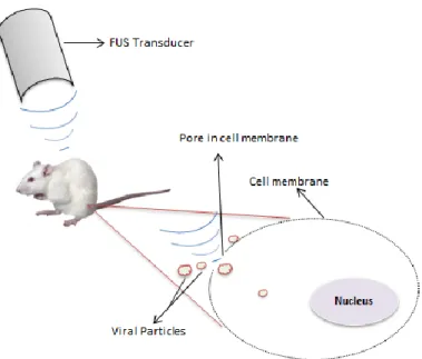
Figure 1.1. Schematic of the Focused Ultrasound - mediated viral particles delivery by sonoporation ... 36 Figure 2.1. Schematic diagram of the beam plotting system... 55 Figure 2.2. Ultrasound pressure profiles in Y (in MPa) as a function of Distance from focus (in mm) at drive levels of 166.7, 333.3, 500, 666.7 and 833.4 mV (from top to bottom). Prms corresponds to the RMS pressure, P max and P min correspond to peak positive and peak negative pressures, respectively. Nonlinearity can be seen at the highest drive levels where Pmax > Pmin ... 57 Figure 2.3. Ultrasound beam profiles in X as the Pressure (in MPa) as the function of Distance from focus (in mm) at the drive levels of 166.7, 333.3, 500, 666.7 and 833.4 mV (from top to bottom). Prms corresponds to the RMS pressure, P max and P min correspond to peak positive and peak negative pressures, respectively. Nonlinearity can be seen at the highest drive levels where Pmax > Pmin ... 58 Figure 2.4. More extensive ultrasound beam plot in Y axis at the drive level of 1V and drive frequency of 1.08 MHz to check if the main lobe and the side lobes imediately after the main lobe would be inside the well-plates used for in vitro experiments, to be sure that at least 80% of the energy of the beam would be used. ... 59 Figure 2.5. Longer ultrasound beam plot in X axis at the drive level of 1V and drive frequency of 1.08 MHz to check if the main lobe and the side lobes imediately after the main lobe would be inside the well-plates used for in vitro experiments, to be sure that at least 80% of the energy of the beam would be used. ... 59 Figure 2.6. Pressure (in MPa) plotted as a function of the Drive Level (in mV) at 1.08 MHz. ... 59

(12)

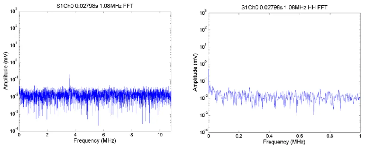
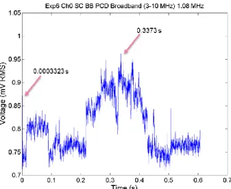
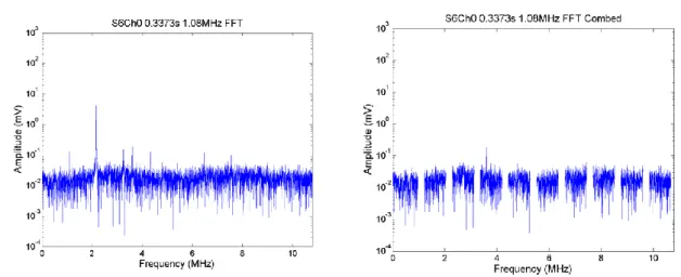
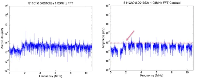
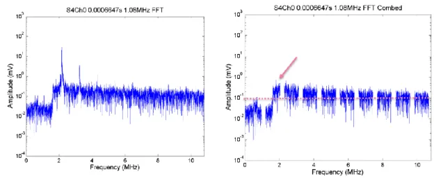
Figure 2.7. Pressure (in MPa) plotted as a function of the Drive Level (in mV) at 1.34 MHz. ... 60 Figure 2.8. Pressure (in MPa) plotted as a function of the Drive Level (in mV) at 1.66 MHz. ... 60 Figure 2.9. Schematic of well-plate built in house (left) and photograph (right). The volume of each well was approximately 0.5ml. The diameter is just under 7 mm wide which meant that if the 1.66 MHZ transducer was used the beam should just clear the sides of the well when the focal peak is placed in the middle of the well (in 3D). ... 63 Figure 2.10. Radiotherapy Platform used to move the ultrasound transducer automatically and precisely from well to well. ... 64 Figure 2.11. Example for setup to exposures in vitro (the tank is filled with degassed water prior to any exposure). The well-plate holder is holding a standard 96 well plate, which could not be used for US exposures because the thick perspex was not acoustically transparent and the plate could not be totally submerged. This means that there would be almost complete reflection of the ultrasound beam at the liquid air interface in each well and so, ultrasound exposure levels could not be accurately measured. ... 64 Figure 2.12. PCD broadband signal (frequency-integrated over 3-10 MHz) as a function of time for a single 1.08 MHz, 0.5 s exposure of DMEM with peak negative pressure 0 MPa. The exposure lasts 0.5 s of acquisition. No cavitation was detected, because no exposure was made. Therefore in this case the whole trace represents off-time noise of the entire PCD detection system. The graph title shows that this was exposure number one, with data acquired on Ch0 of the DAQ system. ... 69 Figure 2.13. FFTs from a single segment of PCD data at 0.2798 s obtained during an 1.08 MHz, 0.5s exposure of DMEM. The FFTs show noise level broadband , only data between 3 to 10 MHz are summed, (left) and half harmonic at 0.504 MHz (right) of noise level. The peak value of this off-time noise is around 0.03 (3 x 10^-2). The title shows the exposure number (S1) and that data recorded channel 0 on the DAQ were processed ... 69 Figure 2.14. PCD broadband signal (3-10 MHz) as a function of time for a 1.08 MHz, 0.5s exposure of DMEM at a peak negative pressure of 1.5 MPa. The arrows show time points that were identified for analysis in the frequency domain because of their transiently increased amplitude above off-time noise. ... 70 Figure 2.15. FFTs from a single segment of PCD data from a 1.08MHz, 0.5s exposure in DMEM. The whole FFT (left) and harmonic comb-filtered FFT are shown (right). To compute the broadband level the data between 3 and 10 MHz would be summed. ... 70 Figure 2.16. FFTs from a single segment of PCD data from a single exposure in DMEM. The FFTs show broadband component (left) and comb filtered broadband (right). ... 71

(13)

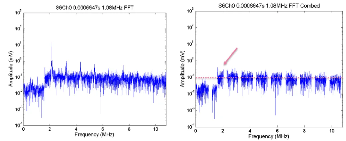
Figure 2.17. PCD broadband signal integrated over the band of 3-10 MHz as a function of time for a single exposure in DMEM with 10% concentration of microbubbles at a peak negative pressure of 0.3 MPa. The arrows show the time points analysed in the frequency domain. ... 71 Figure 2.18. FFTs from a single segment of PCD data from a single exposure at 0.3 MPa in DMEM with 10% concentration of microbubbles. The FFTs show broadband component (left) and harmonic comb filtered broadband (right). ... 72 Figure 2.19. FFTs from a single segment of PCD data from a single exposure at 0.3 MPa in DMEM with 10% concentration of microbubbles. The FFTs show broadband component (left) and harmonic comb filtered broadband (right). ... 72 Figure 2.20. PCD broadband signal integrated over the band of 3-10 MHz as a function of time for a single exposure in DMEM with 10% concentration of microbubbles at a peak negative pressure of 0.9 MPa. The arrows show the time points analysed in the frequency domain. ... 73 Figure 2.21. FFTs from a single segment of PCD data from a single exposure in DMEM with 10% concentration of microbubbles at 0.9 MPa. The FFTs show broadband component (left) and harmonic comb filtered broadband (right). Comparing this to the off-time noise (over 3-10 MHz), there is a clear elevation and broadband, suggesting this could well be cavitation. ... 73 Figure 2.22. PCD broadband signal integrated over the band of 3-10 MHz as a function of time for a single exposure in DMEM with 10% concentration of microbubbles at a peak negative pressure of 1.2 MPa. The arrow shows a time point analysed in the frequency domain. ... 74 Figure 2.23. FFTs from a single segment of PCD data from a single exposure in DMEM with 10% concentration of microbubbles. The FFTs show broadband component (left) and harmonic comb filtered broadband (right). ... 74 Figure 2.24. PCD broadband signal integrated over the band of 3-10 MHz as a function of time for a single exposure in DMEM with 20% concentration of microbubbles at a peak negative pressure of 0.6 MPa. The arrows points towards a time points chosen to analyse in the frequency domain. ... 75 Figure 2.25. FFTs from a single segment of PCD data from a single exposure in DMEM with 20% concentration of microbubbles. The FFTs show broadband component (left) and harmonic comb filtered broadband (right). ... 75 Figure 2.26. PCD broadband signal integrated over the band of 3-10 MHz as a function of time for a single exposure in DMEM with 20% concentration of microbubbles at a peak negative pressure of 0.9 MPa. The arrow show a time point chosen to analyse in the frequency domain. ... 76

(14)

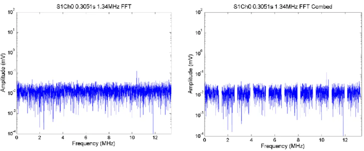
Figure 2.27. FFTs from a single segment of PCD data from a single exposure in DMEM with 20% concentration of microbubbles. The FFTs show broadband component (left) and harmonic comb filtered broadband (right). Comparing this to the off-time noise (over 3-10 MHz), there is a clear elevation and broadband, suggesting this could well be cavitation. ... 76 Figure 2.28. PCD broadband signal (frequency-integrated over 3-10 MHz) as a function of time for a single 1.34 MHz, 0.5 s exposure of DMEM with peak negative pressure 0 MPa. The last 0.1 s of acquisition is the off-time noise. No cavitation was detected, because no exposure was made. Therefore in this case the whole trace represents off-time noise of the entire PCD detection system. The graph title shows that this was exposure number one, with data acquired on Ch0 of the DAQ system. Average noise is 0.655 ± 0.051 mV, and highest noise is ~0.7 mV. ... 77 Figure 2.29. FFTs from a single segment of PCD data from a single exposure in DMEM. The FFTs show broadband component (left) and harmonic comb filtered broadband (right). FFTs from a single segment of PCD data at 0.3051 s obtained during an 1.34 MHz, 0.5s exposure of DMEM. The FFTs show noise level broadband , only data between 3 to 10 MHz are summed, (left) and comb filtered broadband (right) of noise level. The peak value of this off-time noise is around 0.03 (3 x 10^-2). The title shows the exposure number (S1) and that data recorded channel 0 on the DAQ were processed ... 77 Figure 2.30. PCD broadband signal integrated over the band of 3-10 MHz as a function of time for a single exposure in DMEM at a peak negative pressure of 1.06 MPa. The arrows show the time points chosen to analyse in the frequency domain. ... 78 Figure 2.31. FFTs from a single segment of PCD data from a single exposure in DMEM. The FFTs show broadband component (left) and harmonic comb filtered broadband (right). ... 78 Figure 2.32. PCD broadband signal integrated over the band of 3-10 MHz as a function of time for a single exposure in DMEM with 10% concentration of microbubbles at a peak negative pressure of 0.21 MPa. The arrow shows a time point analysed in the frequency domain. ... 79 Figure 2.33. FFTs from a single segment of PCD data from a single exposure in DMEM with 10% concentration of microbubbles. The FFTs show broadband component (left) and harmonic comb filtered broadband (right). ... 80 Figure 2.34. PCD broadband signal integrated over the band of 3-10 MHz as a function of time for a single exposure in DMEM medium with 10% concentration of microbubbles at a peak negative pressure of 0.64 MPa. The arrows show a time point chosen to analyse in the frequency domain through FFT. ... 80

(15)

Figure 2.35. FFTs from a single segment of PCD data from a single exposure in DMEM with 10% concentration of microbubbles. The FFTs show broadband component (left) and harmonic comb filtered broadband (right). Comparing this to the off-time noise (over 3-10 MHz), there is a clear elevation and broadband, suggesting this could well be cavitation. ... 81 Figure 2.36. PCD broadband signal integrated over the band of 3-10 MHz as a function of time for a single exposure in DMEM with 20% concentration of microbubbles at a peak negative pressure of 0.64 MPa. The arrow points towards a time point chosen to analyse in the frequency domain. ... 82 Figure 2.37. FFTs from a single segment of PCD data from a single exposure in DMEM with 20% concentration of microbubbles. The FFTs show broadband component (left) and harmonic comb filtered broadband (right). Comparing this to the off-time noise (over 3-10 MHz), there is a clear elevation and broadband, suggesting this could well be cavitation. ... 82 Figure 2.38. PCD broadband signal (frequency-integrated over 3-10 MHz) as a function of time for a single 1.66 MHz, 0.5 s exposure of DMEM with peak negative pressure 0 MPa. No cavitation was detected, because no exposure was made. Therefore in this case the whole trace represents off-time noise of the entire PCD detection system. The graph title shows that this was exposure number one, with data acquired on Ch0 of the DAQ system. Average noise is 0.730 ± 0.0941 mV, and highest noise is ~0.8 mV. ... 83 Figure 2.39. FFTs from a single segment of PCD data from a single exposure in DMEM. The FFTs show broadband component (left) and harmonic comb filtered broadband (right) of noise level. ... 83 Figure 2.40. PCD broadband signal integrated over the band of 3-10 MHz as a function of time for a single exposure in DMEM at a peak negative pressure of 1.8 MPa. The arrow points towards a time point chosen to analyse in the frequency domain. ... 84 Figure 2.41. FFTs from a single segment of PCD data from a single exposure in DMEM. The FFTs show broadband component (left) and harmonic comb filtered broadband (right). ... 84 Figure 2.42. PCD broadband signal integrated over the band of 3-10 MHz as a function of time for a single exposure in DMEM with 20% concentration of microbubbles at a peak negative pressure of 0.3 MPa. The arrow points towards a time point chosen to analyse in the frequency domain. ... 85 Figure 2.43. FFTs from a single segment of PCD data from a single exposure in DMEM with 10% concentration of microbubbles. The FFTs show broadband component (left) and harmonic comb filtered broadband (right). ... 85

(16)

Figure 2.44. PCD broadband signal integrated over the band of 3-10 MHz as a function of time for a single exposure in DMEM with 10% concentration of microbubbles at a peak negative pressure of 0.6 MPa. The arrow points towards a time point chosen to analyse in the frequency domain. ... 86 Figure 2.45. FFTs from a single segment of PCD data from a single exposure in DMEM with 10% concentration of microbubbles. The FFTs show broadband component (left) and harmonic comb filtered broadband (right). Comparing this to the off-time noise (over 3-10 MHz), there is a clear elevation and broadband, suggesting this could well be cavitation. ... 86 Figure 2.46. PCD broadband signal integrated over the band of 3-10 MHz as a function of time for a single exposure in DMEM with 20% concentration of microbubbles at a peak negative pressure of 0.6 MPa. The arrow points towards a time point chosen to analyse in the frequency domain. ... 87 Figure 2.47. FFTs from a single segment of PCD data from a single exposure in DMEM with 20% concentration of microbubbles. The FFTs show broadband component (left) and harmonic comb filtered broadband (right). Comparing this to the off-time noise (over 3-10 MHz), there is a clear elevation and broadband, suggesting this could well be cavitation. ... 87 Figure 3.1. Schematic of the design of exposures. The arrows show examples of different conditions used to study the effect of pressure on BN175 cell culture. In each well-plate only 3 conditions were tested in order to guarantee the quality of the results. Other designs were tested but the error bars associated with each result were too big to allow a valid conclusion. ... 94 Figure 3.2. Results from 3 independent experiments on viability of cells only, exposed to different levels of pressure. Error bars shown are the standard deviation for each sample (n=8) at the different drive levels used. ... 96 Figure 3.3. Results from 3 independent experiments on viability of cells only exposed to different levels of pressure 1 day after exposure. Error bars shown are the percentage of standard deviation of each sample (n=8) for the different drive levels used. ... 96 Figure 3.4. Results from 3 independent experiments on viability of cells only exposed to different levels of pressure 3 days after exposure. Error bars shown are the percentage of standard deviation of each sample (n=8) for the different drive levels used. ... 97 Figure 3.5. Results from 3 independent experiments on viability of cells only exposed to different levels of pressure with 1% concentration of microbubbles in the sample, on the day of exposure. Error bars shown are the percentage of standard deviation of each sample (n=8) for the different drive levels used. ... 98

(17)

Figure 3.6. Results from 3 independent experiments on viability of cells only exposed to different levels of pressure with 1% concentration of microbubbles in the sample, 1 day after exposure. Error bars shown are the percentage of standard deviation of each sample (n=8) for the different drive levels used ... 99 Figure 3.7. Results from 3 independent experiments on viability of cells only exposed to different levels of pressure with 1% concentration of microbubbles in the sample, 3 day after exposure. Error bars shown are the percentage of standard deviation of each sample (n=8) for the different drive levels used ... 99 Figure 3.8. Results from 3 independent experiments on viability of cells only exposed to different levels of pressure with 10% concentration of microbubbles in the sample, on the day of exposure. Error bars shown are the percentage of standard deviation of each sample (n=8) for the different drive levels used. ... 100 Figure 3.9. Results from 3 independent experiments on viability of cells only exposed to different levels of pressure with 10% concentration of microbubbles in the sample, 1 day after exposure.. Error bars shown are the percentage of standard deviation of each sample (n=8) for the different drive levels used. ... 100 Figure 3.10. Results from 3 independent experiments on viability of cells only exposed to different levels of pressure with 10% concentration of microbubbles in the sample, 3 day after exposure. Error bars shown are the percentage of standard deviation of each sample (n=8) for the different drive levels used. ... 101 Figure 3.11. Results from 3 independent experiments on viability of cells in the absence and presence of microbubbles and exposed to different levels of pressure - on the day of treatment. Each line plotted corresponds to the mean of the results of the 3 independent experiments done under different concentrations of microbubbles. Error bars have been left off for clarity of the results. ... 102 Figure 3.12. Results from 3 independent experiments on viability of cells in the absence and presence of microbubbles and exposed to different levels of pressure – 1 day after the treatment. Each line plotted corresponds to the mean of the results of the 3 independent experiments done under different concentrations of microbubbles. Error bars have been left off for clarity of the results. ... 102 Figure 3.13. Results from 3 independent experiments on viability of cells in the absence and presence of microbubbles and exposed to different levels of pressure – 3 days after the treatment. Each line plotted corresponds to the mean of the results of the 3 independent experiments done under different concentrations of microbubbles. Error bars have been left off for clarity of the results... 103 Figure 3.14. Results from 3 independent experiments on viability of cells only exposed with different Pulse Repetition Frequencies on the day of exposure. The levels of PRF

(18)

used are 10, 100 and 1000 Hz Error bars shown are the percentage of standard deviation of each sample (n=8) for the different drive levels used ... 103 Figure 3.15. Results from 3 independent experiments on viability of cells only exposed to different levels of Pulse Repetition Frequency 1 day after exposure. The levels of PRF used are 10 100 and 1000 Hz. Error bars shown are the percentage of standard deviation of each sample (n=8) for the different drive levels used ... 104 Figure 3.16. Results from 3 independent experiments on viability of cells only exposed to different levels of Pulse Repetition Frequency 3 days after exposure. The levels of PRF used are 10 100 and 1000 Hz. Error bars shown are the percentage of standard deviation of each sample (n=8) for the different drive levels used ... 104 Figure 3.17. Results from 3 independent experiments on viability of cells only exposed to different levels of Pulse Repetition Frequency on the day of exposure with 10% concentration of microbubbles in solution. The levels of PRF used are 10 100 and 1000 Hz. Error bars shown are the percentage of standard deviation of each sample (n=8) for the different drive levels used ... 105 Figure 3.18. Results from 3 independent experiments on viability of cells only exposed to different levels of Pulse Repetition Frequency 1 day after exposure with 10% concentration of microbubbles in solution. The levels of PRF used are 10 100 and 1000 Hz. Error bars shown are the percentage of standard deviation of each sample (n=8) for the different drive levels used ... 105 Figure 3.19. Results from 3 independent experiments on viability of cells only exposed to different levels of Pulse Repetition Frequency 3 days after exposure with 10% concentration of microbubbles in solution. The levels of PRF used are 10 100 and 1000 Hz. Error bars shown are the percentage of standard deviation of each sample (n=8) for the different drive levels used ... 106 Figure 3.20. Results from 3 independent experiments on viability of cells in the absence and presence of microbubbles and exposed under different levels of pulse repetition frequency – day of the treatment. Each line plotted corresponds to the mean of the results of the 3 independent experiments done under different concentrations of microbubbles. Error bars are omitted for effects of clarity of results. ... 106 Figure 3.21. Results from 3 independent experiments on viability of cells in the absence and presence of microbubbles and exposed under different levels of pulse repetition frequency – 1 day after the treatment. Each line plotted corresponds to the mean of the results of the 3 independent experiments done under different concentrations of microbubbles. Error bars are omitted for effects of clarity of results... 107 Figure 3.22. Results from 3 independent experiments on viability of cells in the absence and presence of microbubbles and exposed under different levels of pulse repetition frequency – 3 days after the treatment. Each line plotted corresponds to the mean of the

(19)

results of the 3 independent experiments done under different concentrations of microbubbles. Error bars are omitted for effects of clarity of results... 107 Figure 3.23. Results from 3 independent experiments on viability of cells only exposed to ultrasound during 0.5, 5 and 10 seconds on the day of exposure. Error bars shown are the percentage of standard deviation of each sample (n=8) for the different drive levels used. ... 108 Figure 3.24. Results from 3 independent experiments on viability of cells only exposed to ultrasound during 0.5, 5 and 10 seconds, 1 day after exposure. Error bars shown are the percentage of standard deviation of each sample (n=8) for the different drive levels used. ... 108 Figure 3.25. Results from 3 independent experiments on viability of cells only exposed to ultrasound during 0.5, 5 and 10 seconds, 3 days after exposure. Error bars shown are the percentage of standard deviation of each sample (n=8) for the different drive levels used. ... 109 Figure 3.26. Results from 3 independent experiments on viability of cells only exposed to ultrasound during 0.5, 5 and 10 seconds with 10% concentration of microbubbles in solution, on the day of exposure. Error bars shown are the percentage of standard deviation of each sample (n=8) for the different drive levels used. ... 110 Figure 3.27. Results from 3 independent experiments on viability of cells only exposed to ultrasound during 0.5, 5 and 10 seconds with 10% concentration of microbubbles in solution, 1 day after exposure. Error bars shown are the percentage of standard deviation of each sample (n=8) for the different drive levels used. ... 110 Figure 3.28. Results from 3 independent experiments on viability of cells only exposed to ultrasound during 0.5, 5 and 10 seconds with 10% concentration of microbubbles in solution, 3 days after exposure. Error bars shown are the percentage of standard deviation of each sample (n=8) for the different drive levels used. ... 111 Figure 3.29. Results from 3 independent experiments on viability of cells in the absence and presence of microbubbles and exposed to different exposure duration – day of the treatment. Each line plotted corresponds to the mean of the results of the 3 independent experiments done under different concentrations of microbubbles. Error bars are omitted for clear reading of the results. ... 112 Figure 3.30. Results from 3 independent experiments on viability of cells in the absence and presence of microbubbles and exposed to different exposure duration – 1 day after the treatment. Each line plotted corresponds to the mean of the results of the 3 independent experiments done under different concentrations of microbubbles. Error bars are omitted for clear reading of the results. ... 112

(20)

Figure 3.31. Results from 3 independent experiments on viability of cells in the absence and presence of microbubbles and exposed to different exposure duration – 3 days after the treatment. Each line plotted corresponds to the mean of the results of the 3 independent experiments done under different concentrations of microbubbles. Error bars are omitted for clear reading of the results. ... 113 Figure 3.32. Results from 3 independent experiments on viability of cells only exposed to different levels of Duty Cycle on the day of exposure. Error bars shown are the percentage of standard deviation of each sample (n=8) for the different drive levels used. ... 113 Figure 3.33. Results from 3 independent experiments on viability of cells only exposed to different levels of Duration of Exposure 1 day after exposure. Error bars shown are the percentage of standard deviation of each sample (n=8) for the different drive levels used. ... 114 Figure 3.34. Results from 3 independent experiments on viability of cells only exposed to different levels of Duration of Exposure 3 days after exposure. Error bars shown are the percentage of standard deviation of each sample (n=8) for the different drive levels used. ... 114 Figure 3.35. Results from 3 independent experiments on viability of cells only exposed to different levels of Duty Cycle with 10% concentration of microbubbles in solution, on the day of exposure. Error bars shown are the percentage of standard deviation of each sample (n=8) for the different drive levels used. ... 115 Figure 3.36. Results from 3 independent experiments on viability of cells only exposed to different levels of Duration of Exposure with 10% concentration of microbubbles in solution, 1 day after exposure. Error bars shown are the percentage of standard deviation of each sample (n=8) for the different drive levels used. ... 116 Figure 3.37. Results from 3 independent experiments on viability of cells only exposed to different levels of Duration of Exposure with 10% concentration of microbubbles in solution, 3 days after exposure. Error bars shown are the percentage of standard deviation of each sample (n=8) for the different drive levels used. ... 116 Figure 3.38. Results from 3 independent experiments on viability of cells in the absence and presence of microbubbles and exposed under different duty cycle – day of the treatment. Each line plotted corresponds to the mean of the results of the 3 independent experiments done under different concentrations of microbubbles. Error bars are omitted for clear reading of the results. ... 117 Figure 3.39. Results from 3 independent experiments on viability of cells in the absence and presence of microbubbles and exposed under different duty cycle – 1 day after the treatment. Each line plotted corresponds to the mean of the results of the 3 independent

(21)

experiments done under different concentrations of microbubbles. Error bars are omitted for clear reading of the results. ... 118 Figure 3.40. Results from 3 independent experiments on viability of cells in the absence and presence of microbubbles and exposed under different duty cycle – 3 days after the treatment. Each line plotted corresponds to the mean of the results of the 3 independent experiments done under different concentrations of microbubbles. Error bars are omitted for clear reading of the results. ... 118 Figure 3.41. Study on the effects of pressure on DMEM. Medium was exposed to ultrasound under different drive levels of pressure and then cells were added to the exposed medium to verify if they would attach and grow compared to control (same number of cells added to unexposed medium). Error bars shown are the percentage of standard deviation of each sample (n=8) for the different drive levels. ... 119 Figure 3.42. Flow cytometric analysis of control BN175 cells (not exposed to ultrasound) in DMEM with 20% SonoVue Microbubbles. From top to bottom, first a dot plot shows the counts of the cells in terms of size (x axis) and shape (y axis). The gate (placed around the green dots) defines the population of interest – live cells; then, an histogram shows the counts of emissions detected by the filter 610/20nm(L1)-PI, which is the filter used to distinguish populations with/without PI; finally, a table of statistics gives useful information on the populations – from all the events detected, the population of interest was identified and then inside this population P2 and P3 distinguish the populations without and with PI, respectively. The definition of P2 and P3 was made with data from controls with PI (Figures 3.45-3.47). The gates are fixed for all the analysis. ... 121 Figure 3.43. Flow cytometric analysis of BN175 cells exposed to ultrasound at peak negative pressure of 0.6 MPa in DMEM with 20% concentration of SonoVue microbubbles. From top to bottom, first a dot plot shows the counts of the cells in terms of size (x axis) and shape (y axis). The gate (placed around the green dots) defines the population of interest – live cells; then, an histogram shows the counts of emissions detected by the filter 610/20nm(L1)-PI, which is the filter used to distinguish populations with/without PI; finally, a table of statistics gives useful information on the populations – from all the events detected, the population of interest was identified and then inside this population P2 and P3 distinguish the populations without and with PI, respectively. The definition of P2 and P3 was made with data from controls with PI (Figures 3.45-3.47). The gates are fixed for all the analysis. ... 122 Figure 3.44. Flow cytometric analysis of BN175 cells exposed to ultrasound at peak negative pressure of 1.8MPa in DMEM with 20% concentration of SonoVue microbubbles. From top to bottom, first a dot plot shows the counts of the cells in terms of size (x axis) and shape (y axis). The gate (placed around the green dots) defines the population of interest – live cells; then, an histogram shows the counts of emissions detected by the filter 610/20nm(L1)-PI, which is the filter used to distinguish populations with/without PI; finally, a table of statistics gives useful information on the populations

(22)

– from all the events detected, the population of interest was identified and then inside this population P2 and P3 distinguish the populations without and with PI, respectively. The definition of P2 and P3 was made with data from controls with PI (Figures 3.45-3.47). The gates are fixed for all the analysis. ... 123 Figure 3.45. Flow cytometric analysis of unexposed BN175 cellsin DMEM with 20% concentration of SonoVue microbubbles. From top to bottom, first a dot plot shows the counts of the cells in terms of size (x axis) and shape (y axis). The gate (placed around the green dots) defines the population of interest – live cells; then, an histogram shows the counts of emissions detected by the filter 610/20nm(L1)-PI, which is the filter used to distinguish populations with/without PI; finally, a table of statistics gives useful information on the populations – from all the events detected, the population of interest was identified and then inside this population P2 and P3 distinguish the populations without and with PI, respectively. The gates are fixed for all the analysis. Clear distinction of two populations help in the definition of P2 (green) and P3 (blue). The gates are fixed in all the analysis. ... 124 Figure 3.46. Flow cytometric analysis of BN175 cells exposed to ultrasound at a peak negative pressure of 0.6MPa in DMEM with 20% concentration of SonoVue microbubbles. From top to bottom, first a dot plot shows the counts of the cells in terms of size (x axis) and shape (y axis). The gate (placed around the green dots) defines the population of interest – live cells; then, an histogram shows the counts of emissions detected by the filter 610/20nm(L1)-PI, which is the filter used to distinguish populations with/without PI; finally, a table of statistics gives useful information on the populations – from all the events detected, the population of interest was identified and then inside this population P2 and P3 distinguish the populations without and with PI, respectively. The gates are fixed for all the analysis. ... 125 Figure 3.47. Flow cytometric analysis of BN175 cells exposed to ultrasound at a peak negative pressure of 0.6MPa in DMEM with 20% concentration of SonoVue microbubbles. From top to bottom, first a dot plot shows the counts of the cells in terms of size (x axis) and shape (y axis). The gate (placed around the green dots) defines the population of interest – live cells; then, an histogram shows the counts of emissions detected by the filter 610/20nm(L1)-PI, which is the filter used to distinguish populations with/without PI; finally, a table of statistics gives useful information on the populations – from all the events detected, the population of interest was identified and then inside this population P2 and P3 distinguish the populations without and with PI, respectively. The gates are fixed for all the analysis. ... 126 Figure 4.1. On the left (1) - Schematic of Isolated Limb Perfusion Technique in a rat: a – Soft Tissue Sarcoma; b- perfusion reservoir; c- roller pump; d-tourniquet. Adapted from: Wilfred K. de Roos et al, “Isolated Limb Perfusion for Local Gene Delivery - Efficient and Targeted Adenovirus-Mediated Gene Transfer Into Soft Tissue Sarcomas”, Annal of Surgery, 2000, 232(6), p. 814-821; On the right (2) – Superposition of photos from the

(23)

ILP system used. The yellow arrows point to the components labelled in figure 4.1.1. ... 129 Figure 4.2. Cannulation of Blood Vessels: a- incision in the groin; b- dissected vessels cannulated. The yellow band is a rubber band used to retract the inguinal ligament (not present in the figure). ... 130 Figure 4.3. Picture of the PCD holder, built in-house, and placed around the VIFU 2000 dry transducer, inside a water bag full of degassed water, to provide coupling . The orange arrow points to the ring that fixes the holder to the transducer. the yellow arrow indicates the piece of the holder that allows movement of the PCD in two directions for positioning and the red arrow points tothe piece of the design that holds the PCD in place. ... 131 Figure 4.4. Beamplotting of Y axes of VIFU 2000 dry system transducer at a power level of 4.8 W ... 132 Figure 4.5. Beamplotting of X axes of VIFU 2000 dry system transducer at a power level of 4.8 W ... 132 Figure 4.6. Data from VIFU2000 calibration at different power levels using an hydrophone and the micrometric gantry to positioning effects. Only one measurement was done due to lack of time so there are no error bars present. Specifications sheet from NPL sets the error of the hydrophone detection to 7% but a value of 10% of error in each measurement is considered to avoid underestimates ... 133 Figure 4.7. Photo showing the experimental arrangement, including the water bag used for effects of coupling. A - The leg of the rat is roughly centered under the plastic film which is transparent to ultrassound. B – A rat is positioned under the water bag, the VIFU transducer is positioned just above the leg and the computer on the right shows what the imaging probe is detecting. The computer contains a software that allows treatment planning. ... 134 Figure 4.8. Alpinion’s Focal Field Map in two orthogonal directions – x and z. ... 135 Figure 4.9. Brown Norwegian Rats were used for the in vivo experiments of the pilot study were anesthetized, operated in to cannulate the femoral artery and vessel ... 137 Figure 4.10. Brown Norwegian Rats used for the in vivo experiments of this pilot study were positioned on the VIFU 2000 operating table, a water bag filled in with degassed water was placed on top ... 137 Figure 4.11. After the experiments, the rats were sutured, kept in a cage and medicated to minimise any suffering and either 1 or 72h post experiment, they were euthanized and the tumor and organs have been collected and stored to later analysis. ... 137

(24)

Figure 4.12. Expression of the A21L vaccinia gene as measured by qPCR using the Genelux GL-LC1 VV-A21L kit. The viral copy number was normalised using the weight of the tumour samples to give the number of viral copies per gram of tissue. ... 138 Figure 4.13. Pictures from the VPAs of two different cohorts – a cohort without exposure to ultrasound (Standard ILP) and a cohort with the combined treatment at 150W of exposure. There are three wells per sample. The first well is the undiluted lysate from the tumour (Neat) followed by 1 in 100 and 1 in 1000 dilutions of the lysate. The positive control is the stock of virus used at the same dilution for each perfusion. ... 139 Figure 4.14. On top (left), PCD broadband signal (frequency-integrated over 3-10 MHz) and (on right) Half Harmonic signal (integrated around 0.75 MHz) as a function of time for a single 1.5 MHz, 10 s exposure of Brown Norwegian Rats at a peak negative pressure of ~7 MPa. The exposure lasts 10 s and there is cavitation detection during 6.3s. On bottom (left), combed FFTs from a single segment of PCD data at the time point 0.4955 s of the exposure. The FFTs show signal above the threshold for inertial cavitation as defined in Chapter 2. On bottom (right) half harmonic detection at 0.75 MHz with no half harmonic present. The title shows the exposure number (S2) and that data recorded channel 0 on the DAQ were processed. ... 143 Figure 4.15. On top (left), PCD broadband signal (frequency-integrated over 3-10 MHz) and (on right) Half Harmonic signal (integrated around 0.75 MHz) as a function of time for a single 1.5 MHz, 10 s exposure of Brown Norwegian Rats at a peak negative pressure of ~10 MPa. The exposure lasts 10 s and there is cavitation detection during 6.3s. On bottom (left), combed FFTs from a single segment of PCD data at the time point 5.0026 s of the exposure. The FFTs show signal above the threshold for inertial cavitation as defined in Chapter 2 and black arrows point towards the spikes coming from ultra harmonics. On bottom (right) half harmonic detection at 0.75 MHz with half harmonic present and circled in red. The title shows the exposure number (S21) and that data recorded channel 0 on the DAQ were processed. ... 144 Figure 4.16. On top (left), PCD broadband signal (frequency-integrated over 3-10 MHz) and (on right) Half Harmonic signal (integrated around 0.75 MHz) as a function of time for a single 1.5 MHz, 10 s exposure of Brown Norwegian Rats at a peak negative pressure of ~10 MPa. The exposure lasts 10 s and there is cavitation detection during 6.3s. The graph title shows that this was exposure number two, with data acquired on Ch0 of the DAQ system. On bottom (left), combed FFTs from a single segment of PCD data at the time point 5.0026 s of the exposure. The FFTs show signal above the threshold for inertial cavitation as defined in Chapter 2 and black arrows point towards the spikes coming from ultra harmonics. On bottom (right) half harmonic detection at 0.75 MHz with half harmonic present and circled in red. ... 145 Figure 4.17. Ultrasound Imaging acquired in the prior (left) and post (right) exposure to ultrasound on rats 9 , 11 and 20 from cohort 1. The images were acquired using the E-Cube 9 provided with the VIFU system with a phased array transducer working at 10

(25)

MHz. The yellow cross marks the starting point of the treatment – the initial target. Then, a grid of 9 points centred on this point was exposed.. In each grid, the exposure were created from left to right in three rows of three points. ... 147 Figure 4.18. Ultrasound Imaging acquired in the prior (left) and post (right) exposure to ultrasound on rats 10, 12, 21 from cohort 2.. The images were acquired using E-Cube 9 system from Alpinion with a phased array transducer working at 10 MHz. ... 148 Figure 4.19. Ultrasound Imaging acquired in the prior (left) and post (right) exposure to ultrasound on rats 18, 22 and 23 from cohort 3. The images were acquired using E-Cube 9 system from Alpinion with a phased array transducer working at 10 MHz. ... 149

(26)

List of Tables

Table 1. Acoustic Pressure Data from Alpinion’s Calibration in two orthogonal directions – x and z……….135 Table 2. Summary of the information collected from cavitation data processing and analysis of cohort 1 (ILP + 10% MB + FUS at 50W with TNFa in perfusate)……...…..141 Table 3. Summary of the information collected from cavitation data processing and analysis of cohort 2 (ILP + 10% MB + FUS at 150W with TNFa in perfusate)…..…….141 Table 4. Summary of the information collected from cavitation data processing and analysis of cohort 3 (ILP + 10% MB + FUS at 150W)………141

(27)

List of Acronyms

FUS: Focused Ultrasound MB: Microbubbles

ILP: Isolated Limb Perfusion PNP: Peak Negative Pressure PRF: Pulse Repetition Frequency DC: Duty Cycle

DE: Duration of Exposure US: Ultrasound

PCD: Passive Cavitation Detection PZT: Piesoelectric

OA: Oncolytic Adenoviruses OD: Optical Density

P1: Population 1 P2: Population 2 P3: Population 3

VPAs: Viral Plaque Assays SD: Standard Deviation

TNF-α: Tumour Necrosis Factor-alpha

qPCR: real-time quantitative Polimerase Chain Reaction RFP: Red Fluorescet Protein

GFP: Green Fluorescent Protein

(28)

1. Introduction

Chapter by Chapter Overview

1.1.1. Chapter 1 – Introduction to Transducers Calibration

The Introductory part of this thesis is divided in sections such as i) “Motivation and Background”, in which there is a brief description of the main concepts and of the project itself, ii) Hypothesis and Thesis Aim”, where the hypothesis is that Focused UltraSound (FUS) in the presence of MicroBubbles (MB) enhances the activity of oncolytic virotherapy delivered during Isolated Limb Perfusion (ILP) through several mechanisms which include direct anti-tumour activity and enhancement of the activity of melphalan/TNF-α and increased intratumoural delivery of oncolytic viruses. For this, the FUS fields to be used will be characterised using well established techniques. In vivo experiments will be made in Brown Norwegian Rats implanted with fibrosarcoma cells (BN175 cell line) and then an overview on, iii) Virotherapy for Cancer, iv) Focused Ultrasound in Cancer Therapies, v) Basic Principles of FUS, vi) Cellular interaction mechanisms in therapies using Focused Ultrasound which will help to clarify the main concepts used along this dissertation. Finally, vii) the state of the art of combined treatments using drugs/virus and focused ultrasound that describes the last decade studies on the area of oncolytic virotherapy combined with FUS.

1.1.2. Chapter 2 – Calibration of a Focused Ultrasound Transducer

and Measurement of Cavitation Thresholds under Different

Frequencies

This chapter is divided into two main sections. The first section describes the ultrasound beam, its propagation and the processes involved in Transducers Calibration. There are three sub-sections for Transducers Calibration: an introduction, then the methodology used and finally the results. The second part of this chapter has to do with the Measurement of Cavitation Thresholds at three different drive frequencies. A Brief

(29)

Review on the topic is the first sub-section and this is followed by the description of the Methods and then the Results which are presented paired with the Discussion of the Results.

1.1.3. Chapter 3 - In Vitro Study on the Effects of Focused Ultrasound

on BN175 Sarcoma Cell Line

This chapter focuses on the potential of ultrasound and microbubbles to enhance drug delivery by the process of Sonoporation, i.e. the formation of temporary pores in the cell membrane, as well as enhanced Endocytosis that have been reported as the main biological mechanisms involved. In general, the uptake of drugs or small molecules is attributed to ultrasound mediated transient permeabilization of the cell membrane. This transient permeabilization can occur due to stable and inertial cavitation events in the presence or absence of artificial microbubbles. To confirm this, physical parameters of ultrasound such as Peak Negative Pressure (PNP), Pulse Repetition Frequency (PRF), Duty Cycle (DC) and Duration of Exposure (DE) have been tested at different levels to see how this could affect the fibrosarcoma cell line. The Methodoly used is described and a Discussion of the Results helps to take some conclusions.

1.1.4. Chapter 4 - In Vivo Study on the Development of a Combined

Treatment for Cancer using Virus and Focused Ultrasound

The toxicity of viral therapy is a concern and to minimize it, a novel technique known as Isolation Limb Perfusion has been developed. This is a chemotherapeutic technique using melphalan, Tumour Necrosis Factor-alpha (TNF-α), oncolytic vaccinia virus and involving the cannulation of the blood vessels feeding the tumour-bearing region and isolation of the limb from the systemic circulation by tourniquet mainly due to the severe toxicity of TNF-α. ILP is used in this project, which aims to study the combination of ILP and FUS in the presence of microbubbles to increase viral penetration of tumour bulk in Brown Norwegian rats transfected with BN175 fibrosarcoma cells. The

in vivo work is described in Chapter 4 and this includes a short introduction, the

description of methods and then the presentation of the results and its discussion.

1.1.5. Chapter 5 - Conclusions and Future Work

(30)

This chapter helps to summarize all the conclusions from the experiments of this pilot project but also, contains some important suggestions on what could have been done better and what could be done in the future.

Motivation and Background

Sonoporation is a process by which the permeability of a membrane is changed. This alteration in the membrane generates a passage through which small molecules can enter. During the last decades, research on focused ultrasound and microbubble mediated virotherapy has been carried out and proved to be a good approach to cancer treatment. The treatments under research include strategies such as viral transduction of tumour cells with ‘suicide genes’, using viral infection to trigger immune-mediated tumour cell death and using oncolytic viruses for their direct anti-tumour action.

For oncolytic viruses, sonoporation seems to be important to get increased viral uptake in cells but the safety and efficiency of the overall process needs to be studied for clinical use. The toxicity of viral therapy is a concern and to minimize it, a novel technique known as Isolated Limb Perfusion has been developed. This is a chemotherapeutic technique involving the cannulation of the blood vessels feeding the tumour-bearing region and isolation of the limb from the systemic circulation by tourniquet. ILP will be used in this project in Brown Norwegian rats transfected with BN175 Fibrosarcoma cells. A Fibrosarcoma is malignant soft tissue tumor or sarcoma that usually grows in the lower extremities of the human body. Treatment for a fibrosarcoma involves a wide excision, usually combined with radiation therapy. In severe cases of fibrosarcoma, it might be necessary to remove the entire limb to guarantee the survival of the patient.

Research must be done to diminish the invasiveness of tumor therapies. This project is a pilot study based on a study of Pencavel et al. which is entitled as “Isolated limb perfusion with melphalan, tumour necrosis factor-alpha and oncolytic vaccinia virus improves tumour targeting and prolongs survival in a rat model of advanced extremity sarcoma” that was published in 2015 in the International Journal of Cancer. So, the aim is to add Focused Ultrasound to this combined therapy to see i) if there is an increased uptake and replication of virus for enhanced efficacy of the treatment and ii) if there is a

(31)

possibility to avoid the use of tumour necrosis factor-alpha, which is toxic when in the systemic circulation, to reduce the invasiveness of the treatment.

The main goals of this pilot project are to study tumor virus distribution and then to quantify the number of viral particles in the tumors using appropriate assays (e.g. qPCR, Plaque Assay, Immunofluorescence). This will involve in vitro experiments with the BN175 rat sarcoma line, initially to test a combination therapy with the virus in the presence or absence of (i) focused ultrasound (ii) microbubble and (iii) focused ultrasound and microbubbles.

The physical parameters to be optimised are peak negative pressures, duty cycle, pulse repetition frequency, exposure duration and microbubble concentration. Once a range of optimal parameters has been found, these will be applied in in vivo Brown Norwegian rats in order to determine if a combined therapy using Focused Ultrasound, Melphalan, TNF-α and Vaccinia Virus using the technique of ILP. TNF-α is a cell signaling protein (cytokine) involved in systemic inflammation that is also capable of induce fever, apoptotic cell death, and inhibit tumorigenesis and viral replication. This molecule is mortal in the concentration it is used in this therapy so it will also be studied the possibility to avoid this chemotherapeutic agent to reduce the toxicity of the treatment.

Contributions

The hypothesis to be tested was that Focused Ultrasound in the presence of microbubbles enhances the efficacy of oncolytic virotherapy delivered during Isolated Limb Perfusion through several mechanisms, which include direct anti-tumour activity, enhancement of the activity of melphalan/TNF-alpha, and increased intratumoural delivery of oncolytic viruses.

The following specific research aims were addressed:

1. Characterisation (in vitro and in vivo) of the effects of FUS and MB on standard ILP with melphalan/TNF-alpha in rat distal limb sarcoma.

2. Evaluation of FUS + MB over a range of ultrasound intensities as a means of enhancing intratumoural delivery of oncolytic virotherapy during ILP. These studies included the evaluation of viral biodistribution using viral plaque assays, quantitative PCR, analysis of gene expression and non-invasive imaging (bioluminescent and GFP/RFP imaging), – characterisation of the effects of

(32)

therapeutic FUS + MB with ILP-delivered oncolytic virotherapy. These studies involved the evaluation of the effects of treatment schedule and dose and included

in vivo (direct measurement, imaging analysis).

The FUS fields used were characterised using well established techniques and the ultrasound parameters investigated were peak negative pressures, duty cycle, Pulse repetition frequency, and duration of exposure. These parameters were varied with the aim of identifying the conditions that gave the optimal viability for the sarcoma cell line used (BN175 cell line). These were investigated in combination with commercially available ultrasound contrast agents (i.e. MB) in an attempt to find the most effective exposure. The mechanisms for any observed effects were studied. Ultrasonic cavitation was monitored, and its influence investigated.

The therapeutic efficacy of FUS/MB-assisted oncolytic virotherapy during ILP, this was tested in immunocompetent brown Norwegian rats bearing BN175 syngeneic tumours. These models allowed evaluation of effects of the combination therapy on locoregional control.

Virotherapy for Cancer

The possibility of treating the underlying causes instead of solely its symptoms, and thus eliminating disease, is getting closer and closer to reality when we talk about cancer. Research is being undertaken in the field of viral based gene delivery systems and has already proved to be useful for the treatment of some tumors [1-4].

Over the last century, clinicians have already used a spectrum of wild-type viruses to treat cancer patients. However this approach was temporarily abandoned not only due to adverse biological effects of the virus and to safety of both patients and staff, but also because of enthusiasm for the advent of chemotherapy [5]. Over the past decade, research in this field has once again been taking place, with several viruses having been evaluated. Genetic engineering of viruses to target cancers safely is now a few steps away from worldwide clinical application - the first agent is about to be approved for use as a novel cancer therapy modality [6, 7].

(33)

The use of oncolytic viruses in oncology is called virotherapy, and nowadays is one of the most promising cancer therapy methods. Viral-mediated gene delivery systems consist of site-specific delivery of viruses which are modified to be replication-deficient outside the target tissue, but which can deliver DNA for expression. In this context, viruses can be used as anti-cancer agents which attack malignant cells, while healthy cells remain relatively undamaged. Different kinds of viral vector systems are used, including retrovirus, adenovirus, adeno-associated virus, herpes simpex virus or lentivirus [8]. As well as having an anti-cancer effect, oncolytic viruses are also capable of inducing an anti-tumour immune response – immunotherapy – which is thought to help in eliminating residual cancer cells or in maintaining micrometastases in a state of dormancy [9].

Adenoviral vectors are the most promising and widely used platform for gene therapy and virotherapy. However, there have been problems associated with their use [10]. The major challenges in adenovirus-mediated cancer gene therapy and virotherapy are poor transduction in human tumors, and the existence of immune responses against the adenovirus that drastically limit the vector transduction efficiency and the duration of transgene expression [11]. In order to avoid these problems, several strategies have been proposed, these include the modification of the viral particles to provide increased affinity to tumor receptors, and to facilitate binding and replication, and the use of immunosuppressive agents to eliminate a possible anti-viral immune response [10-12]. Others goals, which focus on treatment efficacy, are to obtain specificity to cancer cells (in order to avoid damaging normal cells), and improvement in the means of inducing cell death by modifying viral proteins to destroy cancer cells by promotion of viral replication in malignant cells but not in normal cells, thus enabling the targeting of metastastic cancer cells. A third goal in terms of efficiency is to improve transduction – the delivery of therapeutic genes into cancer cells. The overall efficacy of the treatment of tumors with viral particles can also be enhanced if combined with methods that help to open the membranes of cancer cells [11, 12].

There are tumor specific viral vectors which are equipped with an efficient delivery system, and are ready for immediate use in in vivo mouse models, and for testing in clinical trials, but still can not be used to treat patients on a regular basis. The therapy most used to treat tumours is chemotherapy. It helps to shrink tumors but this is usually reversible – the tumors can grow again and become resistant to the treatment. This resistance can be reduced if chemotherapy is combined with other treatments which rely