M
ASTER IN
ACTUARIAL SCIENCE
M
ASTERS
F
INAL
W
ORK
I
NTERNSHIP
R
EPORT
M
ETHODS OF
C
APITAL
A
LLOCATION IN A
S
OLVENCY
II
E
NVIRONMENT
R
AQUEL
S
EQUEIRA
C
ORREIA
i
M
ASTER IN
ACTUARIAL SCIENCE
M
ASTERS
F
INAL
W
ORK
I
NTERNSHIP REPORT
M
ETHODS OF
C
APITAL
A
LLOCATION IN A
S
OLVENCY
II
E
NVIRONMENT
R
AQUEL
S
EQUEIRA
C
ORREIA
S
UPERVISORS:
C
ARLAS
ÁP
EREIRAH
UGOB
ORGINHOii
Abstract
Under Solvency II regulation the SCR is mainly calculated using a standard formula
which considers the risks that an insurer faces. Due to this aggregation of risks, a
diversification benefit is achieved and the global SCR is smaller than the sum of the
capital requirements of each risk. To take these diversification benefits into
account the total capital should be allocated back to the lower levels of risk by
applying a proper method of capital allocation. This report is the result of a
curricular internship that took place at EY. One of the goals was to find the most
appropriate method to perform a capital allocation of the SCR of an insurance
company. Five methods of allocation were studied, Proportional,
Variance-Covariance, Merton and Perold, Shapley and Euler. The methods were compared
theoretically by analyzing their respective properties, and based on several studies
in the literature it is concluded that the Euler method is the most appropriate to
apply. This report contributes to a better understanding of capital allocation
methods and allows to demonstrate how to allocate the SCR. It also contributes to
show how to construct the SES for the purpose of the calculation of the adjustment
of LAC DT. Since this task was one of the difficulties enumerated in the Fifth
Quantitative Impact Study (QIS 5), this work can serve as a literary base, being
useful to overcome these difficulties.
Keywords: Solvency II; SCR; capital allocation; Proportional method;
Variance-Covariance method; Merton and Perold method; Shapley method; Euler method;
iii
Resumo
De acordo com a regulamentação de Solvência II, o SCR é geralmente calculado
usando uma fórmula padrão que considera os riscos que uma seguradora enfrenta.
Devido à agregação dos diferentes riscos, são originados benefícios de
diversificação e um valor de SCR total menor que a soma dos requisitos de capital
de cada risco. Para ter em conta estes benefícios de diversificação, o capital total
deve ser alocado de volta aos níveis mais baixos de risco, aplicando um método
apropriado de alocação de capital. Este relatório é resultado de um estágio
curricular que decorreu na EY. Um dos objetivos foi encontrar o método mais
apropriado para realizar a alocação do SCR de uma empresa de seguros. Foram
estudados cinco métodos de alocação, Proporcional, Variância-Covariância, Merton
e Perold, Shapley e Euler. Os métodos são comparados teoricamente, analisando as
suas respetivas propriedades e, com base em vários estudos presentes na
literatura, conclui-se que o método de Euler é o mais apropriado. Este trabalho
contribui para uma melhor compreensão dos métodos de alocação de capital e
permite demonstrar como alocar o SCR. Contribui também para mostrar como
construir o SES para fins do cálculo do ajustamento LAC DT. Visto que esta tarefa
foi uma das dificuldades referidas no QIS 5, este trabalho pode servir como base
literária, sendo útil para superar essas dificuldades.
Palavras-chave: Solvência II; SCR; alocação de capital; método Proporcional;
método de Variância-Covariância; método de Merton e Perold; método de Shapley;
iv
Acknowledgements
I would like to thank my supervisor at EY, Carla Sá Pereira, for her guidance and
availability to clarify any questions that arose throughout my internship. I also
thank the entire Actuarial team that always showed the willingness and patience to
help me throughout the process, with special attention to Vanessa Serrão, who
guided a large part of my tasks during the internship and with whom I had the
opportunity to learn a lot.
I am grateful to my supervisor at ISEG, Professor Hugo Borginho, for the support
and care for my work, giving me essential guidelines and advices for the
preparation of my internship report. I also thank Professor Maria de Lourdes
Centeno for helping me find this excellent curricular internship opportunity.
Finally, I thank my family and friends especially those who shared with me the day
to day while I was studying or writing this work.
I am grateful to my boyfriend who has been on my side for years giving me support
and encouraging me to achieve my goals.
To my parents who have always believed in me and have been giving me
continuous encouragement throughout my life and years of study, I am deeply
grateful and there are no possible words to describe all the unconditional support
v
Contents
Abstract... ii
Resumo ... iii
Acknowledgements ... iv
List of Figures ... vii
List of Tables ... viii
Acronyms and Abbreviations ...x
1. Introduction ... 1
2. Bibliographic review ... 3
3. Risk Measures ... 4
3.1 Value at Risk (VaR) ... 5
3.2. Tail Value at Risk (TVaR) ... 6
4. Solvency II ... 8
4.1 Introduction ... 8
4.2 Solvency Capital Requirements ... 9
5. Risk capital allocation ...11
5.1 Introduction to the capital allocation problem ...11
5.2 Properties of risk capital allocation methods ...13
5.3 Proportional allocation ...14
vi
5.5. Merton-Perold Allocation ...15
5.6. Shapley Allocation ...16
5.7. Euler Allocation ...18
5.8. Choice of method ...19
6. Case Study ...23
6.1. Data and data treatment ...23
6.2. Euler Allocation ...26
6.3. Comparison of Euler Allocation with other methods...28
7. Why allocate capital? ...32
7.1 Single Equivalent Scenario and Loss absorbing capacity of technical provisions and deferred taxes ...32
8. Conclusion ...35
References ...36
Appendix ...41
A. Data ...41
B. Correlation between risks ...43
vii
List of Figures
viii
List of Tables
Table 6.1.1: Capital per line of business for P&R of Health NSTL risk submodule...25
Table 6.1.2: Capital requirements for Premium, Reserve, and P&R of Health NSLT risk submodule. ...25
Table 6.2.1: Results of Euler capital allocation method per module of risk...27
Table 6.2.2: Results of Euler capital allocation method for the Market risk module. ...27
Table 6.2.3: Results of Euler capital allocation method for the Health NSLT risk submodule. ...28
Table 6.3.1: Allocation to lines of business of P&R risk of Health NSLT risk submodule with different methods. ...29
Table 6.3.2: Euclidean distance between Euler and other methods regarding P&R risk of Health NSLT risk submodule. ...30
Table 6.3.3: Euclidean distance between Euler and other methods regarding P&R risk of Non-Life risk module. ...30
Table A.1: Capital requirements. ...41
Table A.2: P&R volumes and the respective standard deviations for each line of business of P&R risk of Health NSLT risk submodule. ...42
Table B.1: Correlations between risk modules ...43
Table B.2: Correlations between submodules of Market risk module. ...43
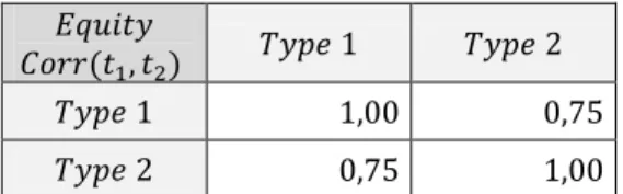
Table B.3: Correlations between equities of type 1 and equities of type 2. ...43
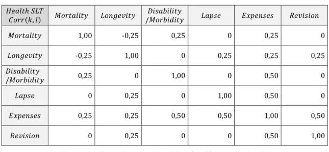
Table B.4: Correlations between submodules of Health risk module. ...43
ix
Table B.6: Correlations between submodules of Health CAT risk submodule. ...44
Table B.7: Correlations between submodules of Health NSLT risk submodule. ...44
Table B.8: Correlations between LoBs of P&R of Health NSLT risk submodule. ...44
Table B.9: Correlations between submodules of Non-Life risk module ...45
Table B.10: Correlations between LoBs of P&R of Non-Life risk module. ...45
Table B.11: Correlations between submodules of Default risk module. ...46
x
Acronyms and Abbreviations
BSCR - Basic Solvency Capital Requirement
CAT - Catastrophe
DT - Deferred taxes
DTA - Deferred tax assets
DTL - Deferred tax liabilities
EIOPA - European Insurance and Occupational Pensions Authority
Eul. - Euler allocation method
LAC - Loss Absorbing Capacity
LAC DT - Loss Absorbing Capacity of Deferred Taxes
LAC TP - Loss Absorbing Capacity of Technical Provisions
LoB - Line of Business
M & P - Merton and Perold allocation method
MCR - Minimum Capital Requirement
P & R - Premium and Reserve
Prop. - Proportional allocation method
QIS5- Fifth Quantitative Impact Study
xi
SCR - Solvency Capital Requirement
SES - Single Equivalent Scenario
Shap. - Shapley allocation method
TP - Technical Provisions
TVaR - Tail Value at Risk
VaR - Value at Risk
1
1. Introduction
This work is the result of a curricular internship at EY - Ernst & Young, S.A. in the
Actuarial services which started on 13th February and ended on 30th June of 2017.
During the internship I was assigned with tasks related with Solvency II and
Pension Funds allowing me to apply many concepts that I have learned from my
masters. Since the theoretical background of the tasks was so different I chose to
write and do some research on one main topic, Capital Allocation, which I found
interesting and that was not so familiar to me in the beginning of the internship.
Additionally I also got the opportunity to get more insight about concepts such as
the Single Equivalent Scenario (SES) approach and the Loss Absorbing Capacity of
Deferred Taxes (LAC DT)1, which connect easily to the concept of capital allocation.
With the new regulation standards implied by Solvency II many rules have been
established with the aim to provide a safe and stable environment for all financial
institutions including insurance companies. Any risk faced by these institutions
should be quantified, managed and reported, which allows an increase of the
stability of the financial system. It is mandatory to determine the amount of capital,
Solvency Capital Requirement (SCR), that an institution needs to hold in order to
remain solvent. There are two possibilities to compute the SCR, using a standard
model or using an internal model if the same is approved and shown to be more
efficient and suitable for the risk profile of a certain insurance company. It is also
possible to determine the risk capital as a combination of both models. In this
paper the standard model is considered entirely. After computing the SCR an
2
important step to take would be its allocation back to each risk module, sub
module or even to each line of business in such a way that the sum of each
individual risk add up to the total risk. This allows to get some knowledge about
the benefits from diversification effects resulting from the aggregation of all risks.
Allocation of capital has many different applications in a financial institution, such
as, the division of capital reserve among business units, support on strategic
decision making regarding new lines of business, for pricing, assessment of
performance of each portfolio and of managers, settlement of risk limits and also
portfolio optimization. For an insurance company the advantages are also many
and similar to the ones stated before and capital allocation methodologies can also
be used to find the SES. To determine the best way to do this, five different
allocation methodologies were studied in order to determine which method could
be more appropriate. In chapter 2 a bibliographic review is provided given that
some conclusions and assumptions in this work were based on previous research
articles. Chapters 3 and 4 give a brief overview about risk measures and Solvency
II regime, chapters 5 and 6 require the most attention, since the risk capital
allocation problem is defined, as well as the different methodologies, its properties
and a theoretical decision about which method to use. Subsequently, the practical
results of the final chosen method are showed and for a particular case all the
methodologies were applied in order to know how different the results were. Also,
some insight about the SES, LAC DT and possible applications of capital allocation
are given in chapter 7. At last, it is possible to find final conclusions and
3
2. Bibliographic review
This chapter provides a summary of the available literature on capital allocation
methods. Several authors have contributed to this area by explaining allocation
methods in detail, or bringing new perspectives and possible applications of it.
Merton and Perold (1993) provides an allocation method that is based on option
pricing theory. The work of Tasche (1999, 2004, 2007,2008) provides a wide range
of information regarding the Euler method and proves that this method is the only
one suitable for measurement of performance. Overbeck (2000) introduced the
Variance-Covariance method. Denault (2001) presents the coherence of an
allocation method and explains the Shapley, Aumann-Shapley and Euler methods.
Urban et al. (2003) compares and analyzes different methods of capital allocation
providing some equivalences between them. Buch and Dorfleitnet (2008) has as a
main topic the coherence of risk measures and allocation methods. More authors
continued to study this topic, for instance, Furmanand Zitikis (2008), Corrigan et
al. (2009), Balog (2011), Dhaene et al. (2012), Gulicka et al. (2012) and Karabey
(2012). Regarding the applications of an allocation method, Cummins (2000),
Panjer (2002), Gründil and Schmeiser (2005), Buch et al. (2011) and Asimit et al.
(2016) provide different ideas and perspectives on the matter. Some conclusions
presented in this report were based on Balog et al. (2017) which also presents
various allocation methods and focus on the properties of coherence that each one
satisfies. EIOPA regulations and guideline papers also provided a strong
4
3. Risk Measures
Artzner (1999), Artzner et al. (1999) and Pitselis (2016) provided the main
theoretical background for this chapter.
Risk can be interpreted in many ways, it can be a possible loss or its variance, a
change in the future values of random variables or a set of events that can cause
loss. An insurance company faces a lot of uncertainties and must be prepared to
face the risks that is exposed to. Therefore, measuring risk is essential to find the
capital that a company should hold is order to be able to face any unexpected
losses. A risk measure assigns a real number to the random variables of a portfolio.
This section gives a brief introduction to risk measures and focus on the two most
known risk measures used by insurance companies.
Let be the set of random variables which represent a set of events that a
portfolio is exposed to and let be a random variable belonging to this set.
Definition 3.1: A risk measure is a mapping from the set of variables to the
real line :
An appropriate risk measure should be consistent with economic and finance
theory so it is important to define some properties that a good risk measure should
satisfy.
Definition 3.2: A risk measure is a coherent risk measure if it satisfies the
following properties:
5
2. Translation invariance:
3. Subadditivity:
4. Monotonicity: If then
Positive homogeneity means that scaling a portfolio implicates the same scaling for
the risk, for instance, double the same portfolio also result on twice the risk.
Translation invariance implies that when adding a determinist amount to the
portfolio, the risk changes by the same amount. Subadditivity is related with the
concept of diversification, that is, merging two or more risks/portfolios does not
generate additional risk. Therefore, diversification of risks is essential in a
portfolio. At last, monotonicity implies that a random variable or a portfolio with
higher and better value (lower losses) originates a lower or equal risk under all
the scenarios.
Besides the risk measure, an insurer must also choose the time period over which
a risk is going to be measured. Under Solvency II, the risk measure used to
determine the Solvency Capital Requirement (SCR) is the Value at Risk with a time
horizon of one year. Another risk measure is the Tail Value at Risk which can be
considered to calculate the economic capital of the company.
3.1 Value at Risk (VaR)
Known as one of the most used risk measures in the financial sector, the VaR is the
maximum loss not exceeded of a given risk over a given time horizon. For a
confidence level , VaR is mathematically defined as
6
Thus, is the quantile of the cumulative distribution of risk
The VaR is positive homogenous, translation invariant and monotone but is not
subadditive in some cases which leads to it not been a coherent risk measure and
the diversification effects in a portfolio of risks may be compromised. Also, the
main disadvantage of using VaR is that, although it measures the maximum
potential loss, it fails to measure the severity of losses that fall above the
confidence level Despite this drawbacks, the computation of VaR is relatively
simple and easy to explain leading to the most preferred risk measure of the
insurers and also the elected measure by the European Commission to determine
the SCR.
3.2. Tail Value at Risk (TVaR)
The Tail Value at Risk is a more robust risk measure than VaR. It can be interpreted
as the mean of the expected losses above the confidence level given that a loss of
that magnitude occurs.
Mathematically,
Therefore, the TVaR provides information about the average of the tail. For normal
distributions the difference between VaR and TVaR is relatively smaller when
compared with other distributions with a heavier tail. The main difference is that
the TVaR is a coherent measure satisfying all the properties and it gives more
7
good approach is to determine the capital requirements with both measures and
analyze if there are any substantial differences. If the difference is small then it
indicates that the tail of the distribution is small and the severity of losses does not
reach values well beyond VaR. Thus, there is no practical reason to use TVaR since
it is a more complicated measure to compute. On the other hand, if the difference is
consider to be relevant then a further research on the matter should be done since
it is possible that some extreme events may lead to adverse situations and
different conclusions, including on capital allocation results. However and as it
was mentioned before, VaR is easier to calculate, easier to explain and it was
8
4. Solvency II
4.1 Introduction
This chapter provides a quick and short explanation about Solvency II regulation,
mentioning only the appropriate concepts for the scope of this work.
This European regulation arose as a way to ensure financial soundness of
insurance undertakings providing more transparency, better management and a
harmonized solvency and supervisory regime for the insurance sector.
Solvency II is divided in three components named "pillars":
Pillar I - Quantitative Requirements: Gives orientations on the minimum
capital requirement (MCR), solvency capital requirement (SCR) based on a
standard approach or an internal/partial model, own funds and
investments.
Pillar II - Qualitative Requirements: Focuses on governance, risk
management and internal control, and supervisory review process.
Pillar III - Disclosure and market discipline: Comprises reporting and
disclosure of information, transparency and harmonized reporting to the
supervisors.
This report requires a special attention to Pillar I, specifically to what is related
9
4.2 Solvency Capital Requirements
The SCR is the level of capital that the insurer is required to hold in order to be
able to face unexpected losses. It is calculated as the Value at Risk with a
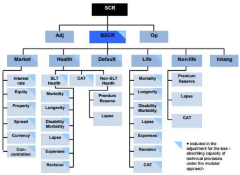
confidence level of 99,5% over one year time horizon. The SCR considers all the
risks that the insurer may face which under Solvency II regulation are organized as
in the following scheme:
Let M= {Market, Health, Default, Life, Non-life} and be the set of risks belonging
to module , .
is the number of risks in module
is the required capital for module
is the required capital for the risk of module ,
is the correlation between modules and ;
is the correlation between risks and .
10 The overall SCR is given by the formula
where is the adjustment for loss absorbing capacity of technical provisions
and deferred taxes ( = ) which takes a null or negative
value and is the capital requirement for Operational risk.
The is the result of the aggregation of the risk modules in which can be
calculated as
In most cases, the capital requirement for each risk module is given by
Intangible and Default risk modules are determined in a different way since they
do not have any submodules. Moreover, the calculation of the capital charges of
each risk sub module is different and to provide more insight on this topic the
reader is advised to consult the Commission Delegated Regulation (EU) 2015/35
and EIOPA-14-322 guideline regarding the capital requirements calculations.
For this work is also important to refer the Premium and Reserve risk for both
Health NSLT and Non-Life risks and explain how the capital charge is determined.
All the formulas and assumptions related to this topic can be consulted in section
6.1 - Data and data treatment.
11
5. Risk capital allocation
5.1 Introduction to the capital allocation problem
When a portfolio is composed by different risk units and its risk capital is
computed with a risk measure, diversification effects are in place. Usually, the sum
of the individual risk contributions of the risk units is larger than the risk capital of
the whole portfolio. Therefore, it is important to allocate the risk capital in a fair
way, to each risk unit, in order to evaluate its contribution to the total
diversification effects.
To provide a more general notation, consider the following definitions for a
portfolio composed by different risks:
, represents the set of all risk units.
, , is a random variable representing the amount of loss due to the
risk unit .
is the aggregate loss of the whole portfolio, dependent on all
the individual losses
is an appropriate risk measure that quantifies the amount of losses at the
level of a risk unit or portfolio and represents the capital necessary to cover
that same risk.
is the risk capital required to hold for unit
is the total risk capital required to hold for the portfolio.
represents the risk capital that is allocated “back”, after
12
In an insurance company, it will be assumed that is the set of all risk
modules, is equivalent to the and is the SCR of the risk module .
The notation can also be extended to the level of risk submodules and lines of
business of an insurance company. The allocation must be backwards, that is, one
should first compute the allocated capital of each module, then use it to compute
the allocated capital to each submodule and only in the end to the lines of business
if applicable.
Following Denault’s (2001) approach, let us defined the allocation problem:
Definition 5.1.1. Let be the set of risk capital allocation problems and (
composed by a set of portfolios and a risk measure . An allocation principle is
a function Π that maps each allocation problem ( into a unique
allocation:
Π
Π Π
Π
Definition 5.1.2: The allocation ratio, also called diversification factor, represents
the portion of capital of a risk unit that was allocated back to that same risk unit.
Mathematically,
Definition 5.1.1 leads to the need to establish which conditions make the function
13
5.2 Properties of risk capital allocation methods
Definition 5.2.1. An allocation Π is a coherent allocation principle if it satisfies the
following properties:
1. Full allocation:
2. No undercut:
3. Symmetry: Let and be two risks that make the same contribution to the
risk capital. If they join any subset then .
4. Riskless allocation: If the unit is riskless with worth 1 at time 0 and
worth at any point T, then and
Full allocation property implies that the sum of the individual allocated capital
amounts add up to the total risk, that is, the capital is fully allocated. No undercut
property means that the standalone allocated capital of a risk or a subset of risks is
smaller than the total risk capital of the whole risk set. Symmetry implies that
identical risks should be treated in the same way. More specifically, when adding
two risks to any disjoint subset which result in the same amount of capital
contribution then the allocated capital should also coincide. Finally, riskless
allocation means that the allocation of a determinist variable, that is, a riskless
component, has no impact on the total capital being allocated to the risk units.
Also, an allocation principle is a non-negative coherent allocation if it satisfies all
the previous properties and if
Additionally, there are also some more properties that can be useful to compare
14
coherence. Namely and according to Balog et al. (2017), the Diversification, Strong
Monotonicity, Incentive Compatibility, Covariance and Decomposition Invariance
properties. It is considered that the violation of a property can occur in theoretical
situations and it might not be relevant in practical situations.
5.3 Proportional allocation
Proportional allocation is the easiest method to be applied where the
diversification effect is proportionally distributed to all the risk units.
The “new” contribution of the risk unit i, is given by the following formula:
This method satisfies the full allocation property but it does not take into account
the dependence structures between risks.
5.4. Variance Covariance Allocation
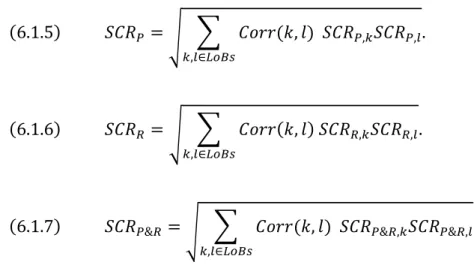
This principle of allocation is given by
Where is the variance of the aggregate loss , that is, of the whole risk
portfolio, and is the covariance between the loss and . Risk units
facing a loss that is more correlated with the total loss are required to hold more
capital than the less correlated. Thus, the method focuses on how each risk unit
contributes to the variance of the portfolio. Depending on the available data, the
15
Where and are the standard deviations of and and is the
correlation between losses and
2
Moreover, relation (5.4.3) proves that the variance of the portfolio can be written
as the sum of the individual covariances between the risks and the whole portfolio
which means that the full allocation property is satisfied.
Given the previous relations and to have the individual risk contributions of each
unit into account, the method can also be written as
5.5. Merton-Perold Allocation
Merton – Perold methodology is an incremental allocation of capital that measures the marginal effect of a risk unit similar to what is done in pricing. Marginal
contributions to the whole portfolio are differences between the total capital
amount of the company including the risk unit and the total capital without risk
unit . Mathematically, the allocated capital is given by
2
16
One disadvantage of this method is that the sum of risk contributions does not add
up to the total capital. A simple alteration solves this problem:
With the previous alteration the full allocation property is now satisfied.
5.6. Shapley Allocation
This methodology can be considered as a general case of the previous method
since in this case the marginal effects of the risk units are studied within all the
possible combinations in a portfolio composed by these risk units.
To illustrate this, consider a group of players working to find the best and fair
coalition possible. The goal is to form a coalition such that all the players benefit
more as a group than as a stand-alone. Game theory provides a solution for a fair
and unique distribution using the Shapley value.
Let denote a coalitional game where is a finite set representing the
number of players and a cost function representing a real number associated to
each subset .
Definition 5.6.1: A value is a function that maps the coalitional game ( into
a unique allocation:
17
Definition 5.6.2: The core of a coalition game is the set of allocations
for which for all coalitions
This ensures that players always form the largest coalition possible since the cost
of each player is always minimized if they join the coalition.
The Shapley value is given by the following formula:
where is the number of players in coalition and is the total number of
players.
According to the previous notation this is equivalent to:
where is the number of risk units in subset and is the total number of existent
risk units.
Hence, this method takes into consideration all permutations of the risk units,
computes the marginal benefit of each unit in each case and returns the allocated
capital as an average of the marginal benefits.
The computation of this method can be extensive and not worthy because the
higher the value of , the higher the number of possible coalitions, leading to a
number of possible combinations to analyze.
There is also an extension of the Shapley value, the Aumann-Shapley value that
18
theory. Although this is not in the scope of this work, is still important to refer
since the next method was derived from this concept.
For further details on Shapley and Aumman-Shapley see Balog (2011), Denault
(2001), Karabey (2012) and Kaye (2015).
5.7. Euler Allocation
The Euler allocation method is also known as the gradient allocation principle and
is currently one of the most used methods. This method can be used under a
differentiable and homogeneous risk measure of degree 1.
Definition 5.7.1: A risk measure is homogenous of degree if for any ,
A function is called homogeneous of degree if for all ,
and
Theorem 5.7.1: Let be an open set and a continuous
differentiable function. The function is homogeneous of degree if and only if,
Let be defined as if equals 1, is a homogeneous risk measure of
degree 1 and according to the theorem 5.7.1 the following equation holds:
19
Remember that and also depends on the variables
leading to the following formula to compute the allocated capital according to
Euler method:
Given these five methods the goal is to find the best one to apply in a portfolio of an
insurance company and specifically to the practical example that is the object of
study of this work.
5.8. Choice of method
The goal of this work was to find the best method to determine the allocated
capital of each risk module, submodule and to the lines of business. The
conclusions in this chapter are based on theoretical assumptions and on many
researches present in the literature. Also consider the following conclusions
assuming that a coherent risk measure was used.
The Proportional allocation method is the simplest method to apply but does not
take into account the dependence structure between risks which is a big drawback
of this method. It does not penalize portfolios that are highly correlated but also, it
does not reward portfolios that improve the diversification effect. For this reason it
is not considered to be a good methodology to perform the allocation of capital in
20
The Variance-Covariance allocation method satisfies the full allocation principle
but the properties of no undercut, symmetry and riskless allocation are not
satisfied. No undercut may fail because the variance is not a subadditive risk
measure meaning that it is possible to have a risk unit (or a set of them) with an
allocated capital bigger than its initial contribution which should not happen. Also,
suppose that two risk units not belonging to any existing subset have the same risk
contribution to the portfolio but a different variance. If they join the subset, the
allocated capital will differ because of the difference in their variances, while it
should be equal to satisfy the symmetry property. For the riskless allocation
property it is straight-forward that if a unit is risk free its variance is equal to zero
leading to an allocated capital also equal to zero. For this reason the riskless
allocation property is not satisfied. Moreover, this method gives more importance
to the variance of the risk units which can be a disadvantage and really not
applicable in practice. For example, most risk modules and submodules do not
have any value defined in the Delegated Regulation for its standard
deviation/variance which leads to the need to model the risks or have more
information about the distribution function associated with each risk. In this work,
all the capital requirements are computed with the standard formula and the only
reference available about standard deviations of risks is for lines of business of
Premium and Reserve submodules of both Non-Life and Health NSLT risk modules.
Thus, it is only possible to apply this method in these particular cases.
Another method considered not the best to apply is the Shapley allocation method.
21
the no undercut property is sometimes violated. Although many researchers
proved that this method, based on game theory, gives good and consistent results
it is not very practical to apply to a whole portfolio. For example, for five risk
modules of an insurance portfolio the number of possible combinations to analyze
is which equals to combinations and since the "order of entrance" in the
portfolio matters to find the final allocated capital of each risk module then
permutations have to be considered in the intermediary calculations. If
the allocation is also done to the lines of business, which was the case, then for the
Premium and Reserve submodule of Non-Life risk module a much more serious
problem is in place. Twelve lines leads to combinations and
479001600 permutations. Looking at this numbers and considering the
chosen tool to perform the allocation of capital (Excel) the decision was to
compare results for a particular case but not to apply this method for the whole
portfolio of the insurance company since it is not practical and the time of
computation is high.
The last two possibilities are Merton and Perold method and Euler method. The
first one satisfies properties of full allocation and symmetry but does not always
satisfy the no undercut and riskless allocation properties. Euler method satisfies
the full allocation, no undercut and riskless allocation properties but fails to satisfy
the symmetry property.
Regarding the previous methods that were studied, none satisfies all properties
that define a coherent allocation principle in a theoretical point of view. Euler
22
properties and is not so complex to compute as the Shapley Value. Furthermore,
researches done on this method refer that it is the most stable to apply even when
considering different risk measures, it is the only method compatible with
portfolio optimization and suitable for performance measurement.
For these reasons the method of capital allocation that was applied to the whole
portfolio of the insurance company was the Euler allocation method. Introduction
and results on the practical problem are present in the next chapter. To compare
this method with the others studied, an extra exercise was performed in order to
23
6. Case Study
The practical component of this work was to apply a method of capital allocation to
allocate the Basic Solvency Capital Requirement (BSCR) to each risk module,
submodule and lines of business of an insurance company, in such way that the
allocated capital sums up to the total BSCR. First in this section is the information
regarding the data available and some calculations that were required before
applying any method. The second part shows some of the results relative to the
application of Euler allocation method, followed by a third section were the Euler
results are compared with all the other methods.
6.1. Data and data treatment
The available data to perform the capital allocation was all the capital
requirements for each risk module and submodules from a composite insurance
company. All the data was anonymized in order to maintain the information about
the client private. Regarding the lines of business only premium and reserve
volumes were provided. Part of this information can be consulted in Appendix A.
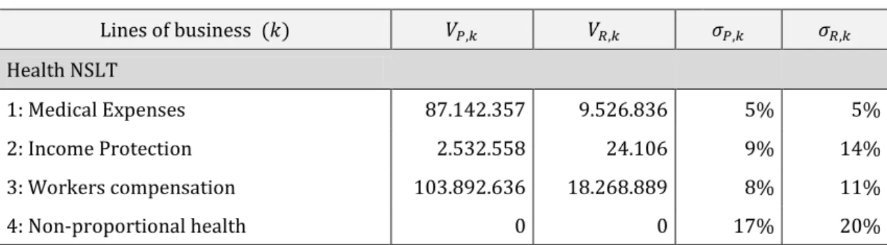
To be able to allocate the capital to each line of business and to Premium Risk and
Reserve Risk separately it was necessary to compute capital charges that can be
interpreted as the SCR for Premium risk and also for Reserve risk for each line of
business, before applying Euler method. To solve this issue the following formulas
were adapted from the ones used in the standard model for the calculation of
premium and reserve risk.
24
Where the represents the Premium component, a Line of Business from the
Premium and Reserve risk submodule and the volume measure of premium
risk of line of business The amounts and are available in the data.
In an equivalent way,
Where the represents the Reserve component, a Line of Business from the
Premium and Reserve risk submodule and the volume measure of reserve risk
of line of business The amounts and are available in the data.
Also,
Where the represents the Premium and Reserve risk submodule and a line
of business. The amount of is calculated with the orientations given by the
Delegated Regulation:
.
With these three formulas it is possible to have a capital charge associated with
each line of business for Premium and Reserve risk and also for both components
in separate. These will be used as the initial risk contributions necessary to apply
Euler method. Another amount that is necessary is the capital associated with the
25
the reserve risk. Using the values obtained is possible to apply the following
formulas:
The last formula must lead to a result equal to the capital requirement for
Premium and Reserve risk submodule given by the insurance company.
The results of this intermediary calculations were calculated for all the lines of
business regarding the Premium and Reserve risk of Health NSLT submodule and
of Non-Life module. As an example, the results related with Health NSLT
submodule can be seen in the following tables.
Table 6.1.1: Capital per line of business for P&R of Health NSTL risk submodule.
Monetary units: Euros
33.815.108 6.861.382 37.702.025
Table 6.1.2: Capital requirements for Premium, Reserve, and P&R of Health NSLT risk submodule.
Monetary units: Euros
26
Notice that the amount is equal to the capital requirement given in the data
for the Premium and Reserve risk of Health NSLT risk submodule. The results are
consistent.
It is now possible to apply Euler allocation method to all the risks components that
the insurance company faces.
6.2. Euler Allocation
The Euler allocation method was applied to all modules of risks, submodules and
lines of business.Remember that the allocation is done backwards and consider
the following notations and formulas that allow the application of this method.
As previously defined, let M= {Market, Health, Default, Life, Non-life} and be the
set of risks belonging to module . Assume always that and
;
It is possible to deduce the amount
which in this case is given by:
3
Therefore, the Euler formula for a risk module is equivalent to:
3 Proof is given in appendix C. Granito and Angelis (2015) also provides a similar approach and
27 For a risk submodule,
Using the same logic it is possible to continue to apply the Euler method to risk
sub-submodules and to lines of business. As an example some of the results are
represented in the next tables.
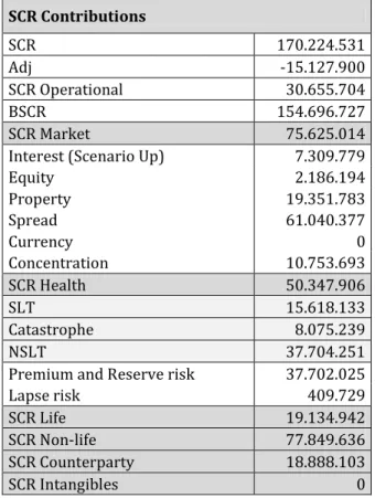
Monetary units: Euros INPUT OUTPUT
SCR Contributions Pre diversification Post diversification
SCR 170.224.531
Adj. 15.127.900
SCROperational 30.655.704 30.655.704
BSCR 154.696.727 154.696.727 Market Risk 75.625.014 57.284.672 Health Risk 50.347.906 25.633.361 Health SLT 15.618.133 5.762.814 Health CAT 8.075.239 1.747.955 Health NSLT 37.704.251 18.122.592 Life Risk 19.134.942 6.846.446 Non-Life Risk 77.849.636 53.444.096 Counterparty/Default Risk 18.888.103 11.488.152
Intangible Risk 0 0
Table 6.2.1: Results of Euler capital allocation method per module of risk.
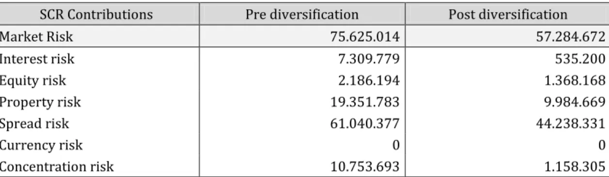
Table 6.2.2: Results of Euler capital allocation method for the Market risk module.
Monetary units: Euros SCR Contributions Pre diversification Post diversification Market Risk 75.625.014 57.284.672 Interest risk 7.309.779 535.200 Equity risk 2.186.194 1.368.168 Property risk 19.351.783 9.984.669 Spread risk 61.040.377 44.238.331
Currency risk 0 0
28
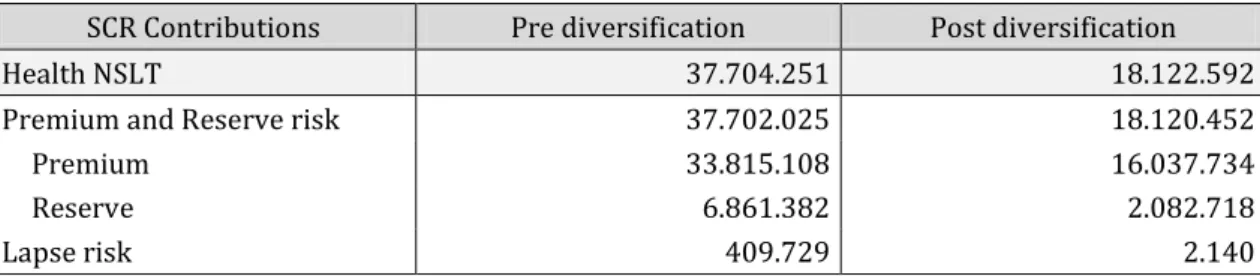
Table 6.2.3: Results of Euler capital allocation method for the Health NSLT risk submodule.
It is possible to see in the previous examples that the full allocation property is
fulfilled and the risk components have an allocated capital lower than the initial
risk contribution. This allows to measure the benefits from diversification effects
resulting from the aggregation of risks.
The allocation of capital was also performed for all lines of business of Premium
and Reserve risk for both Health NSLT submodule and Non-Life module. These
particular cases were chosen to compare the different methods of capital
allocation studied in this work. In the next section it is possible to see an example
regarding to the lines of business of Premium and Reserve Risk of Health NSLT risk
submodule.
6.3. Comparison of Euler method with other methods
This section relates to the comparison of Euler method with the other studied
methods. Since other methods were not applied to all the risk components it was
necessary to assume an allocated capital for the Premium and Reserve Risk for
both Health NSLT and Non-Life risk module. Given that the Euler method is
consider the best method available, the values of the allocated risk capitals for the
Premium & Reserve sub-modules are equal to the ones obtain with Euler principle.
This amounts are used only as a starting point to apply other methods to allocate
the capital to each line of business.
SCR Contributions Pre diversification Post diversification Health NSLT 37.704.251 18.122.592 Premium and Reserve risk 37.702.025 18.120.452 Premium 33.815.108 16.037.734 Reserve 6.861.382 2.082.718
29
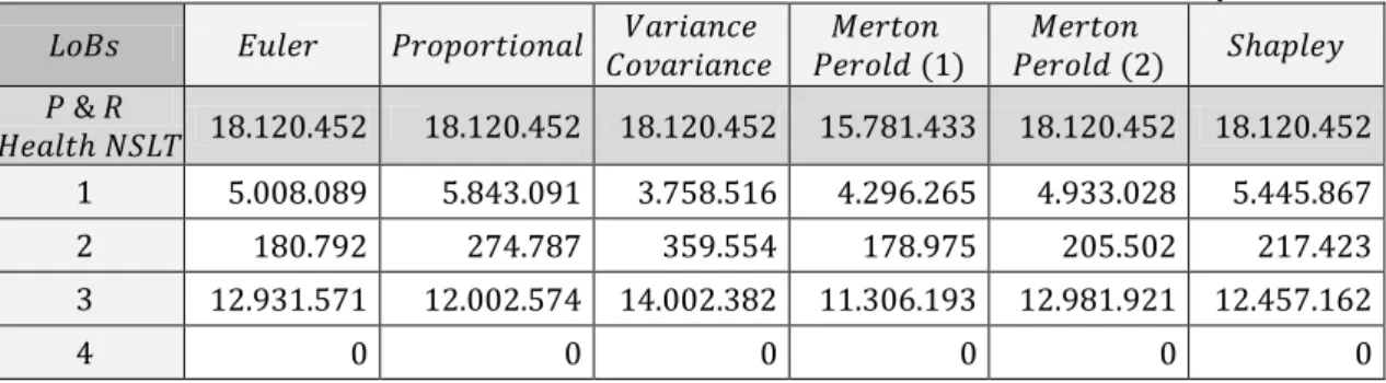
As an example, the allocation to the lines of business of Premium and Reserve risk
of the Health NSLT risk submodule are presented in the next table.
Monetary units: Euros
18.120.452 18.120.452 18.120.452 15.781.433 18.120.452 18.120.452
5.008.089 5.843.091 3.758.516 4.296.265 4.933.028 5.445.867 180.792 274.787 359.554 178.975 205.502 217.423 12.931.571 12.002.574 14.002.382 11.306.193 12.981.921 12.457.162
0 0 0 0 0 0
Table 6.3.1: Allocation to lines of business of P&R risk of Health NSLT risk submodule with different methods.
As it was explained before, Variance Covariance principle is proven not to be a
good choice since is not possible to apply to the other submodules and modules of
risk. Notice that Merton and Perold using formula does not fulfill the full
allocation property as it was expected. However, using formula the
property is now fulfilled and the results seem very similar to the Euler method.
Although is not presented in the example it is important to mention that when
applying the Shapley method to the lines of business of Premium and Reserve risk
of the Non-Life risk module, it was only applied to 9 lines of business due to the
fact that lines 10, 11 and 12 did not have any risk contribution. The first approach
was to construct an excel file able to apply this method to all lines of business and
therefore prepared to receive any data, but the program was constantly shutting
down and also not able to compute all the necessary permutations. Given this
problem, the second tentative was to determine the allocated capital with program
R, even though that was not the chosen tool on which the work had to be done, it
was done to confirm the impossibility to apply Shapley method to 12 lines. Once
30
the method was the most complicate and time-consuming to apply and therefore
not recommended.
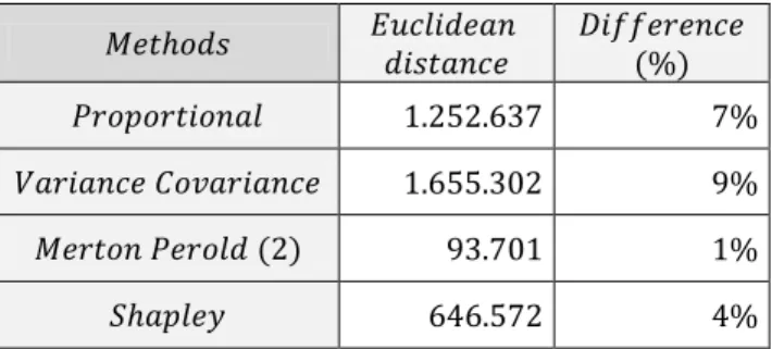
In order to have more insight about the difference between methods the Euclidian
distance was applied.
Definition 6.3.1: Consider a -dimensional space. The Euclidean distance
between two points and is given by:
Euler method is used as a reference. The difference between this method and the
other ones is presented in the next tables.
For the lines of business of Premium and Reserve risk of Health NSLT submodule,
For the lines of business of Premium and Reserve risk of Non-Life module,
1.252.637 7%
1.655.302 9%
93.701 1%
646.572 4%
Table 6.3.2: Euclidean distance between Euler and other methods regarding P&R risk of Health NSLT risk submodule.
5.352.004 12%
3.341.560 8%
685.360 2%
1.878.673 4%
31
As it was expected Proportional allocation and Variance Covariance methods are
the most distant from the Euler method and the Merton Perold method proves to
be the most similar.
Within all the methods studied the preferred method is Euler allocation method
and the most similar to this one is Merton and Perold method (adapted formula).
However, the choice of method should take into account the risk measure, in this
case the risk measure used was VaR which is not a coherent measure of risk.
Theoretically, using TVaR could be more reliable in terms of results because a
coherent risk measure provides a higher chance that the method of allocation is
also coherent and fulfils all the required properties.
Furthermore, the choice of method should be consistent with the purpose of
allocating risk capital, that is, it must be always dependent on the further uses of
32
7. Why allocate capital?
Capital allocation has many applications for the financial institutions. It can be
used for product pricing, for strategic decisions regarding new lines of business, to
decide which lines of business to expand or if a component is worth keeping or not.
Allocating capital is also useful for managing the types of risk a company accepts
and a helpful tool in risk budging, allowing the manager to decide which areas, for
example lines of business, products or even geographical areas, to accept risk. It is
also helpful to evaluate a portfolio performance or even the individual
management performance. In this work the application of a capital allocation
method was needed to find the SES, a concept that is clarified is the next section.
7.1 Single Equivalent Scenario and Loss-absorbing
capacity of technical provisions and deferred taxes
.
The Single Equivalent Scenario (SES) is one of the approaches suggested in the
past by EIOPA, called "alternative approach", to calculate the loss absorbing
capacity (LAC) of technical provisions (TP) and deferred taxes (DT). The SES
assumes a scenario under which all the risks occur simultaneously and regarding
the operational risk, it assumes that the operational loss takes a value equal to the
capital charge of this same risk. To construct this scenario, the capital
requirements for each risk are necessary as inputs. By default, this amounts are the
gross capital requirements, which exactly correspond to the data provided for this
33
represents the 1-in-200 scenario, which can be done by applying a capital
allocation method, for instance, the outputs presented in chapter 6 may be used for
other strategic decisions but also represent the SES for this particular set of data.
Regarding this approach, the following advantages were recognized by EIOPA:
The double counting of LAC TP is avoided.
The LAC DT can also be integrated in the scenario.
More realist management actions.
As for the disadvantages, many undertakings are not familiar with this concept,
referring that it requires more difficult calculations and therefore, this approach
was not extensively tested. In fact, according to CBFA (2011), Central Bank of
Ireland (2011), Dalby (2011), Danish FSA (2011), EIOPA (2011), Financial Services
Authority (2011), Guiné (2011) and Hungarian FSA (2011); countries such as
Belgium, Denmark, Germany, Hungary, Ireland, Norway, Portugal and the United
Kingdom concluded in their QIS5 that only a few participants tried, and some
unsuccessfully, to use the SES approach to calculate the LAC of TP and DT and the
general conclusion was that the calculations are technically very complex. However, this disadvantage can be overcome if there is proper research and
documentation on this matter.
Regarding the LAC DT, some concepts should be clarified just to provide the reader
a brief idea of the following procedures after building the SES.
Deferred taxes (DT) arise from differences between an asset or a liability value, set
for tax purposes, and its SII value. In the SII balance sheet, all items are valued at
their economic value which recognizes unrealized gains/losses, leading to the need
34
represents a liability because it is a tax that is due during the present or has been
assessed but not yet paid. A deferred tax asset (DTA) represents an asset in the
balance sheet that may be used to reduce taxable income, for instance, where there
are any overpaid taxes or taxes paid in advance in the balance sheet, this tax value
will be returned in the future, and therefore may represent an asset.
The loss absorbing capacity of deferred taxes (LAC DT) corresponds to an
adjustment that is equivalent to the change in the net tax position due to the
application of a shock, arising from an instantaneous loss. Building the SES allows
an allocation of this loss to each SII Balance sheet item, that is, an instantaneous
loss can be allocated to the related value of assets and liabilities individually,
resulting on a Balance sheet post shock. After this, is possible to compute the
individual tax adjustments, item by item, which together result on the global
adjustment. The DT aftershock are determined by summing the initial DT and this
global adjustment. The adjustment of LAC DT is therefore, given by the difference
between the value of DT in the SII balance sheet (initial DT) and the value of DT in
the balance sheet post shock (under the SES). The adjustment of LAC DT is only
recognized if the loss leads to a decrease in the DTL or an increase in the DTA. The
decrease in DTL can be immediately recognized for the purposes of the
adjustment, but that is not the case if there is an increase in the DTA, where a
further test must be performed in order to ensure that enough future taxable
income will be available to be used against that assets. Depending on the results of
this test, it is possible that the adjustment for LAC DT has to be narrowed. For
further explanations on the topic, consult CEIOPS (2009) and EIOPA (2014)
35
8. Conclusion
The choice of subject in this report was more specific and since it was more
complex, it was useful to restrict the report to one subject, allowing a greater
understanding and explanation of the topic and all the calculations.
The goal was to find the best capital allocation method to be applied to the SCR.
The proportional allocation is not recommended since it does not take into account
correlations between risks. The variance-covariance method does not satisfy most
of the coherence properties and cannot be used in all modules of risk. The Merton
and Perold method presents results closer to the Euler method, however, it does
not satisfy as many coherence principles as the latter. The Shapley method has the
disadvantage of being difficult to calculate since it is necessary to analyze a high
number of possible combinations between the risk units, resulting in a high
computing time. Finally, the Euler method is the most balanced method between
the ease of its application and the principles of coherence that it satisfies. It is also
well defended by other authors since it is the only appropriate method for
performance measurement. In short, Euler's method is the most recommended to
allocate capital.
For a further research, it would be interesting to perform the allocation under the
two risk measures, VaR and TVaR, to analyze whether the use of a coherent risk
measure affects the results significantly.
In conclusion, this report provides a better understanding of the different
allocations methods and is useful to insurance companies to understand the
36
References
Artzner P. (1999). Application of coherent risk measures to capital requirements in
insurance. North American Actuarial Journal 3 (2), 11- 25.
Artzner, P., Delbaen, F., Eber, J-M., Heath, D. (1999). Coherent measures of risk.
Mathematical Finance 9 (3), 203-228.
Asimit, A. V., Badescu, A. M., Haberman, S., and Kim, E-S. (2016). Efficient risk
allocation within a non-life insurance group under Solvency II Regime.
Insurance: Mathematics and Economics 66, 69-76.
Balog, D. (2011) Capital allocation in financial institutions: the Euler method. Iehas
discussion papers, Institute of Economics, Hungarian Academy of Sciences.
Balog, D., Bátyi, T., Csóka, P., and Pintér, M. (2017). Properties and comparison of
risk capital allocation methods. European Journal of Operational Research
259, 614-625.
Buch, A. and Dorfleitner, G. (2008). Coherent risk measures, coherent capital
allocations and the gradient allocation principle. Insurance: Mathematics and
Economics 42 (1), 235 – 242.
Buch, A., Dorfleitner, G., and Wimmer, M. (2011). Risk Capital Allocation for RORAC
optimization. Journal of Bankink & Finance 35(11), 2001-3009.
CBFA: Banking, Finance and insurance commission (2011). Solvency II Quantitative
Impact Study 5 (“QIS5”) Summary Report for Belgium. Available in:
37
CEIOPS (2009). CEIOPS' Advice for Level 2 Implementing Measures on Solvency II:
SCR standard formula Loss -absorbing capacity of technical provisions and
deferred taxes. CEIOPS-DOC-46/09. Available in:
https://eiopa.europa.eu/CEIOPS-Archive/Documents/Advices/CEIOPS-L2-Final-Advice%20SCR-Loss-absorbing-capacity-of-TP.pdf
CEIOPS (2010). Solvency II Calibration Paper. CEIOPS-SEC-40-10. Available in:
https://eiopa.europa.eu/CEIOPS-Archive/Documents/Advices/CEIOPS-Calibration-paper-Solvency-II.pdf
Central Bank of Ireland (2011). Summary of Irish Industry Submissions for QIS5.
Available in:
http://www.financialregulator.ie/industry-sectors/insurance-companies/solvency2/Documents/Summary%20of%20Irish%20Industry%
20Submissions%20for%20QIS5%20-%20Final%20Report.pdf
Corrigan, J., Decker, J., Delft, L., Hoshino, T., and Verheugen, H. (2009). Aggregation
of risk and Allocation of capital. Milliman. Available in:
http://www.milliman.com/insight/research/insurance/Aggregation-of-risks-and-allocation-of-capital/
Cummins, J. D. (2000). Allocation of Capital in the Insurance Industry. Risk
Management and Insurance Review 3, 7-28.
Dalby, K. (2011). Solvency II: QIS5 for Norwegian Life and Pension Insurance.
Faculty of Mathematic and Natural Sciences, University of Oslo.
Danish FSA (2011). QIS5 Country Report for Denmark. Available in:
https://www.finanstilsynet.dk/~/media/Temaer/2014/Solvens/QIS5-executive-summary.pdf?la=da
38
Dhaene, J., Tsanakas, A., Valdez, E. A., and Vanduffel, S. (2012). Optimal Capital
Allocation Principles. Journal of Risk and Insurance, 79(1), 1-28.
Hungarian Financial Supervisory Authority (2011). QIS5 Country Report for
Hungary. Available in:
https://www.mnb.hu/letoltes/qis5-country-report-public.pdf
EIOPA (2011). EIOPA Report on the fifth Quantitative Impact Study (QIS5) for
Solvency II. EIOPA-TFQIS5-11/001. Available in:
https://eiopa.europa.eu/publications/reports/qis5_report_final.pdf
EIOPA (2014). Final Report on Public Consultation No. 14/036 on Guidelines on
the loss-absorbing capacity of technical provisions and deferred taxes.
EIOPA-BoS-14/177. Available in:
https://eiopa.europa.eu/Publications/Consultations/EIOPA_EIOPA-BoS-14-177-Final_Report_Loss_Absorbing_Cap.pdf
EIOPA (2014). The underlying assumptions in the standard formula for the Solvency
Capital Requirement calculation. EIOPA-14-322. Available in:
https://eiopa.europa.eu/Publications/Standards/EIOPA-14-322_Underlying_Assumptions.pdf
European Union (2015). Regulation - Commission Delegated Regulation (EU)
2015/35 of 10 October 2014 supplementing Directive 2009/138/EC of the
European Parliament and of the Council on the taking-up and pursuit of the
business of Insurance and Reinsurance (Solvency II). Official Journal of the
European Union, L 12, 17. Available in:
39
Financial Services Authority (2011). FSA UK Country Report: The fifth Quantitative
Impact Study (QIS5) for Solvency II. Available in:
https://www.lloyds.com/~/media/files/the-market/operating-at-lloyds/solvency-ii/qis5/qis5_mar11.pdf
Furman, E., and Zitikis, R. (2008). Weighted Risk Capital Allocations. Insurance:
Mathematics and Economics, 43 (2), 263-270
.
Guiné, C. (2011). Solvência II - Resultados do exercício QIS5. Available in:
http://www.asf.com.pt/NR/rdonlyres/052195EE-AF23-4DDD-B225-6167019A726D/0/F31_art1.pdf
Granito, I., and Angelis, P. (2015). Capital allocation and risk appetite under
Solvency II framework. Sapienza University of Rome, Italy.
Gründil, H., and Schmeiser, H. (2005). Capital Allocation for Insurance Companies -
what good is it? Institute of Insurance Economics, University of St. Gallen.
Gulicka, G., Waegenaere, A., and Norde, H. (2012). Excess Based Allocation of Risk
Capital. Insurance: Mathematics and Economics 50, 26-42.
Karabey U. (2012). Risk Capital Allocation and Risk Quantification in Insurance
Companies. School of Mathematical and Computer Sciences, Heriot-Watt
University.
Kaye, P. (2005). Risk Measurement in Insurance: A Guide to Risk Measurement,
Capital Allocation and Relanted Decision Support Issues. Casualty Actuarial
Society Discussion Paper Program. Available in:
https://www.casact.org/pubs/dpp/dpp05/05dpp1.pdf
Merton, R. C., and Perold, A. F. (1993). Theory of Risk Capital in Financial Firms.