I NTERNSHIPR EPORT M ODELLINGR ENEWALP RICEE LASTICITY:ANA PPLICATION TO THEM OTORP ORTFOLIO OFO CIDENTAL

(1)

M

ASTER OF

S

CIENCE IN

A

CTUARIAL

S

CIENCE

M

ASTERS

F

INAL

W

ORK

I

NTERNSHIP

R

EPORT

M

ODELLING

R

ENEWAL

P

RICE

E

LASTICITY

:

A

N

A

PPLICATION TO THE

M

OTOR

P

ORTFOLIO OF

O

CIDENTAL

G

UILHERME

F

ILIPE

P

ALMA

M

OUSINHO

(2)

M

ASTER OF

S

CIENCE IN

A

CTUARIAL

S

CIENCE

M

ASTERS

F

INAL

W

ORK

I

NTERNSHIP

R

EPORT

M

ODELLING

R

ENEWAL

P

RICE

E

LASTICITY

:

A

N

A

PPLICATION TO THE

M

OTOR

P

ORTFOLIO OF

O

CIDENTAL

G

UILHERME

F

ILIPE

P

ALMA

M

OUSINHO

S

UPERVISORS

:

P

ROF

.

D

OUTOR

J

OSÉ

M

ANUEL DE

M

ATOS

P

ASSOS

D

R

.

J

OÃO

F

ILIPE

A

ZEVEDO DOS

S

ANTOS

(3)

Acknowledgements

I would like to thank my supervisor at Ocidental, Filipe Santos, for his indispensable

guidance and availability during this project, along with introducing me to the

capti-vating world of machine learning.

I express my gratitude to my supervisor at ISEG, Professor Jos´e Passos, for his

avai-lability and care for my work.

I am thankful to Professor Lourdes Centeno, for being available to help me secure this

internship.

I am indebted to Sjoerd Smeets and Andr´e Rufino, for providing me with the

oppor-tunity of doing a curricular internship at Ocidental, as well as to the whole Non-Life

Pricing & Business Analytics team, for making me feel like part of it since day one.

I am grateful to Paula Santos, Diana Duarte and Tiago Cavaleiro, for being available

to answer all my questions on the Motor business and much more.

I would also like to thank Rita Costa, for helping me with the inner workings of the

company’s database during the early stages of this project.

(4)

Abstract

The increase in competition in the Portuguese Motor insurance market has lead

insu-rers to consider a more demand-based approach to ratemaking, as a complement to

the usual risk-based approach. Insurance companies now want to have a better

un-derstanding of who their clients are, how they behave, and what actions can insurers

take, during the policy renewal period, in order to prevent their clients from leaving

while maintaining profitability.

This report is the result of a curricular internship that took place at Ocidental

Seguros, with the main goals of modelling the company’s Motor insurance lapse rate

during the renewal period and studying how different covariates influence renewals. We

considered logistic regression, a special case of Generalized Linear Models, to model

the binary response variable renewal/lapse.

By modelling the response as a function of premium change and other covariates,

the lapse probability for each client per amount of premium variation can then be

estimated. As premium change is the only covariate the company has direct control

over, obtaining such knowledge on each client’s price elasticity will allow the insurer

to make better decisions, so that a finer balance between customer satisfaction and

profitability can be achieved.

The model’s capacity to predict which clients will cancel their policy was also

analy-sed. In order to transform the output probabilities into binary classifications, several

threshold optimisation criteria were compared, to find the threshold generating the

best overall discriminatory performance.

(5)

Resumo

O aumento da competitividade no mercado segurador autom´ovel em Portugal tem

levado as seguradoras a considerar uma abordagem de tarifa¸c˜ao mais assente na

pro-cura, como um complemento `a tradicional abordagem baseada no risco. As companhias

de seguros querem actualmente saber mais sobre quem s˜ao os seus clientes, como

es-tes se comportam e que medidas podem as seguradoras tomar, durante o per´ıodo de

renova¸c˜ao de ap´olice, de modo a evitar a sa´ıda dos seus clientes sem prejudicar a

rentabilidade.

Este relatório é o resultado de um estágio curricular que teve lugar junto da

Ociden-tal Seguros, tendo como principais objectivos modelar a taxa de anula¸c˜ao na renova¸c˜ao

do seguro autom´ovel da companhia e analisar como diversas vari´aveis influenciam as

renova¸cões. Considerámos a regressão log´ıstica, um caso particular dos Modelos

Line-ares Generalizados, para modelar a variável de resposta binária renova¸cão/anula¸cão.

Modelando a variável de resposta como uma fun¸cão da varia¸cão do prémio e de

outras variáveis explicativas, é poss´ıvel estimar a probabilidade de anula¸cão por valor

da altera¸cão do prémio para cada cliente. Como a varia¸cão do prémio é a única variável

que a companhia pode controlar directamente, obter tal informa¸c˜ao sobre a elasticidade

pre¸co de cada cliente permitirá à seguradora tomar melhores decisões, com o objectivo

de aperfei¸coar o equil´ıbrio entre o grau de satisfa¸c˜ao dos clientes e a rentabilidade.

A capacidade do modelo em prever que clientes ir˜ao anular as suas ap´olices foi

tamb´em examinada. Para converter as probabilidades obtidas pelo modelo em

classi-fica¸cões binárias, foram comparados vários critérios de optimiza¸cão de ponto de corte,

de modo a encontrar o valor que resulta na melhor capacidade discriminat´oria global.

(6)

List of Figures

3.1 Example of an ROC curve . . . 18

4.1 Calibration plots (both datasets) . . . 24

4.2 Effect of premium change on cancellations . . . 25

4.3 Effect of own damage on cancellations . . . 26

4.4 Effect of claims on cancellations . . . 26

4.5 Effect of payment frequency on cancellations . . . 27

4.6 Lapse probability per conversion rate . . . 28

5.1 ROC curves (both datasets) . . . 30

5.2 Histogram plot (training set) . . . 30

(9)

List of Tables

3.1 Confusion matrix . . . 16

4.1 Difference between observed and estimated lapse rates per cluster (in pp) 24

5.1 Threshold optimisation results (training set) . . . 32

5.2 Application of the chosen threshold (test set) . . . 33

(10)

Chapter 1 Introduction

This Masters Final Work is the result of a curricular internship, which took place

between February and June 2016 at Ocidental Seguros.

When non-life insurance companies develop their pricing strategy, two crucial

mo-ments in their relationship with their clients are taken into account. The first one is

the moment of risk acquisition and signing the contract (conversion). The second one,

which is the focus of this work, is the moment to renew that contract (renewal).

As in most countries, Motor Third-Party Liability insurance is mandatory in

Por-tugal, which has lead to a very competitive Motor insurance market where the average

premium per vehicle systematically decreased over 10 years up to 2014 (Associa¸c˜ao

Portuguesa de Seguradores, 2015). Consequently, very different sets of prices are

avail-able to customers, meaning that, besides the usual risk-based approach to ratemaking,

insurers also need to be very careful with the premium variations presented to

policy-holders, when the time comes to renew their contract. In other words, the increasing

level of competition has compelled insurance companies to start looking into a more

demand-based approach to pricing, by trying to understand who their clients are, how

they behave, and what actions can insurers take, during the policy renewal period, in

order to prevent their clients from leaving while maintaining profitability.

It was under this setting that this work emerged, having as its two main goals

the modelling of the company’s Motor insurance lapse rate and studying how different

covariates influence renewals. By modelling the binary response variable renewal/lapse

as a function of premium change and other covariates, the lapse probability for each

(11)

1. Introduction

As premium change is the only covariate the company has direct control over,

such a model can help the company understand how price elasticity varies from client

to client and what amount of premium change is most adequate for its customers.

Obtaining this knowledge would allow the insurer to make better decisions in order to

achieve a finer balance between customer satisfaction and profitability.

Furthermore, the model can also be adapted to provide predictions of which clients

will cancel their policy. Using these predictions the company could, for instance,

pro-mote proactive retention measures for the customers whose policies were predicted to

be cancelled.

Different approaches to the subject have been studied. Yeo et al.(2001) used

clus-tering and neural networks to model price sensitivities, while more recently Guelman

and Guill´en (2014) have proposed using a causal inference framework, where the

re-sponse isn’t modelled directly. In this work however we followed the more conventional

methodology of using Generalized Linear Models, particularly the special case of

logis-tic regression, to model the response (Bland et al., 1997; Murphy et al., 2000; Guven

and McPhail, 2013).

Although some of the previous works also dealt with the application of the models

in pricing optimisation, our work focused only on the model building and testing

process and on the insights gained from it.

After creating the model, a secondary goal was to evaluate the model’s predictive

capacity and transform its output probabilities into binary predictions. Consequently,

we followed the work of Freeman and Moisen (2008a) by comparing several threshold

optimisation criteria, in order to assess which threshold (above which all policies are

predicted to be cancelled) results in the best overall predictive performance.

The logistic regression approach has also been recently applied by Garraio (2015),

but our work mainly differs in the tests done on the model, the analysis of the model’s

predictive capacity and optimal thresholds, the data (coming from a company

operat-ing in different distribution channels) and the software used.

Regarding the software employed in our work, SAS Enterprise Guide was used for

dataset building and making simple bivariate analyses prior to modelling; Emblem was

used for building the logistic regression model and R was used for testing the model,

evaluating the model’s predictive capacity and optimising thresholds. Use was made of

(12)

1. Introduction

and ‘ggplot2’.

This report is organised as follows. In chapter 2 we discuss the variables used in our

work, describing the response variable and presenting the various covariates analysed.

Chapter 3 begins with an overview of Generalized Linear Models, followed by an

expo-sition of logistic regression and a description of several measures of binary classification

performance. Our modelling strategy and goodness of fit assessment of the model are

presented in chapter 4, followed by a discussion of the more important covariates in

the model. We evaluate the model’s predictive capacity and analyse different

thresh-old optimisation criteria in chapter 5. Our results and suggestions for future work are

(13)

Chapter 2 The data

For the purpose of this work, a training set containing 86 344 policies that went through

the renewal process was built and prepared for modelling, using SAS Enterprise Guide

(Slaughter and Delwiche, 2006). It contains 12 months of data and includes policies

that were up for renewal between March 2015 and February 2016. In addition, a test

set containing 9 714 policies that went through the renewal process in March 2016

was also created, considering the same assumptions and procedures that went into the

creation of the training set. Only individual clients owning passenger cars, commercial

cars or vans were under the scope of this work. For details on the data preparation

stage (the most time consuming part of this work) see section A.1.

In this chapter we start by discussing the response variable in section 2.1. We

present the various covariates in section 2.2, explaining our motivations and

expecta-tions behind them.

2.1 Response variable

For a policy to go through the renewal process, it needs to be in force45 days before the

expiry date of the current term, when the company sends the client a letter indicating

the new premium for the next policy term, in case the client decides to renew. The

policy’s status is then checked 50 days after the expiry date; if it’s still in force it’s

considered to be a renewal, otherwise it’s a cancellation.1

1

This implies that, for a policy with monthly payments, if the client pays the 1st instalment and

(14)

2.2. Covariates

In this work we code the response as 0 if a policy is renewed and as 1 if a policy is

cancelled, meaning that we shall model thelapse or cancellation rate.

Note that, under special circumstances, a policy may be cancelled outside of the

time frame mentioned above. However, as these cancellations aren’t caused by premium

variations they were obviously not considered in our analysis. Keeping the same idea

in mind, policies that were cancelled during that time frame but were motivated by

something certainly not related to premium variations were also discarded from both

datasets.2 _{This includes motives such as total vehicle losses and errors in the company’s}

database.

On the other hand, if a policy was cancelled so that the client could purchase a

new one in the company (policy cannibalisation), it was still kept under analysis as a

cancellation, even though the client hasn’t left the company. This is because this sort

of policy lapse is almost always due to the newer policy having a lower premium for

that customer, so we consider it to be an effect of overpricing on renewals.

2.2 Covariates

In this section we present the different covariates that were included in our datasets,

along with some of our expectations regarding them. Amounting to almost 50

covari-ates, most were suggested in meetings with several key areas in the company dealing

with Motor renewals, such as Actuarial, Underwriting and Marketing. By reviewing

the literature and considering our own intuition, additional ones were added to the list

of variables to analyse. The covariates in our final datasets are marked in bold. For further details see section A.2.

2.2.1 Premium-related covariates

The most important covariate is the premium change, since it’s the only one the

company has direct control over. Thus, we collected for each policy the absolute premium changeand thepercentage premium change. Since these two covariates are obviously correlated, it was decided at start that, when creating the model, testing

would be done to understand which has more explanatory power.

2

(15)

2.2. Covariates

It was discussed whether the full amount of premium being paid should be included

in the list of covariates to analyse since, for example, an increase of AC20 will have

a different impact depending on whether the current premium is AC100 or AC1000.

However, since it’s a function of several rating factors that were also under the scope

of our analysis, the model’s interpretability could be compromised. It was then decided

not to include the current premium in our datasets and, in order to still capture some

of its effect, analyse additional rating factors which weren’t initially considered.

Due to the increasing market competitiveness, it makes sense to account not only

for the company’s own prices but also for the competitors’ prices or, in more general

terms, to how competitive the company’s prices are for different clients. Obviously,

it’s not possible to obtain such information, so it was important to look for a different

way to measure the competitiveness of Ocidental. We followed one of the propositions

given by Murphyet al.(2000) which is to do a conversion analysis, where we estimated

the conversion rate per time of year and customer profile. The motivation behind this idea is that if for a type of client the conversion rates are currently low, then the

company’s price isn’t competitive for those customers and they can find better prices

elsewhere.

It should be noted that using the expected conversion rate as a competitive index

isn’t perfect, as conversion rates reflect how competitive the company is at acquiring

new business, and prices for new customers can be very different from prices for

re-newing clients of the same type (recall that policy cannibalisations weren’t removed

from our analysis). For further details on our conversion analysis see subsection A.2.1.

2.2.2 Customer satisfaction and service levels

In most cases, the customer’s only contact with the company occurs when a policy term

ends and a new one begins. The main exception for this is of course when the client

reports a claim, which is the scenario where the company’s true value presents itself to the client. It was therefore important to analyse whether the client reported a claim

in the previous term and how satisfied they were with the service, as claimants may

focus more on service quality than on premium (Bond and Stone, 2004). Associated

with claims is the level ofbonus-malus discount, which depends on the client’s claim

(16)

2.2. Covariates

To analyse how the company’s service level has an impact on its customers, the

average time to accept a claim and the average time to close a claim were collected, considering only data on Motor claims. To understand how the perception

of service quality by the customers impacts their decision, two Net Promoter Scores

(NPS) (Reichheld, 2003) were used, the claims handling NPSand the call centre NPS (as most clients aren’t claimants but may still contact the company for other reasons).

Still on the topic of customer satisfaction, we observed whether the client had a

rejected claimin the previous term and whether the client made acomplaintin the previous term. Complaints were analysed on a policyholder level and not on a policy

level, as the client’s dissatisfaction with, for example, their Household insurance may

have an impact on their decision to renew the Motor policy.

2.2.3 Client/policy characteristics

Other measures of the relationship between the clients and the company were

inves-tigated. It’s expected that clients that have been with the company for a longer time

are less inclined to cancel their policies, so we collected the policy age and the pol-icyholder’s tenure with the company. Another way to assess customer loyalty is by analysing the number of other policies in force or the number of other lines of business in the company where the clients have policies in force. On the negative side, we collected thenumber of other policies cancelled in the previous term, as we expect that if a client has recently cancelled some other policy then the probability

of cancelling the Motor policy is higher.

Several policy characteristics were also taken into account. An obvious one is the

tariff associated with the policy, as different pricing approaches and retention mea-sures should have a large impact on renewal rates. When analysing Motor policies,

another important factor is whether the policyholder has any own damage cover, since they lead to higher premiums and clients that request them tend to be more

interested in what their insurance provides and more sensitive to claims handling.

Be-sides the previous covariate, we considered thenumber of covers, thesum insured

(17)

2.2. Covariates

number of objects3 _{in the policy and the amount of} _{third-party liability capital}

also made their way into our final datasets.

Another interesting covariate is whether the client made any mid-term changes

to the policy. One example of this may be a policyholder that added own damage

coverage to the policy half way through the term. This policy’s premium has then

increased during the mid-term and the client may only become fully aware of the

amount of this increase during the renewal period, when informed of the new premium

for the full year. The client’s willingness to renew could then decrease.

As for the distribution channel, two levels were considered in this study: “Ban-cassurance” (the company’s main channel) and “Other”. We also looked at the number

of days between the policy issue and start dates, as customers that buy their policy some time before it comes into force may pay more attention to what they’re

buying.

When it comes to the clients themselves, covariates such as their gender and

marital status were analysed. With respect to the former, regulatory constraints prohibit gender-based pricing discrimination, so extra care was taken when dealing

with this covariate.

Regarding ages, besides theclient agewe also kept thedriver agein our datasets. Intuitively, older clients have lower premiums and are financially better off, thus should

be less likely to cancel their policy. The driving licence age, which is usually a rating factor, was analysed as a way to measure the client’s experience in dealing with

insurers.

Covariates related to payments were deemed very important. With respect to the

payment frequency, we anticipate that clients making more payments are less sen-sitive to premium changes, as they don’t feel the variation all at once. Also, clients

paying annually usually only cancel their policy at the end of a policy term (since

they’ve already paid for all of it), so lapse rates for these customers tend to be higher

during the renewal period than for others. As for the payment method, we expect clients paying by direct debit to have a lower cancellation probability, as less effort

goes into making the payments.

Besides the two previous covariates, we looked at whether the client had already

3

(18)

2.2. Covariates

missed paymentsduring the previous term. We considered payments previous to the sending of the letter with the new premium, since failing to make payments is one of

the motives for policy cancellation. Only payments that were missed because the client

couldn’t or didn’t want to pay were taken into account in our work. Still on this topic,

the company has developed a model for classifying customers according to afinancial risk score.

The geographical area where the policyholders live may also offer some

explana-tion for their behaviour during the renewal period. Besides the district, we obtained data from the company’s database on the characteristics of the different postal codes4_,

including covariates such as income deciles, education level deciles, unemploy-ment level and urban-rural classification. A demographic score, using informa-tion from the previous factors and others not considered here, was available per postal

code. The Portugueseunemployment rate (Instituto Nacional de Estat´ıstica, 2016) was also collected and added to the datasets.

Vehicle characteristics were also considered, such as the type of vehicle, the

power-to-weight ratio, theweight, theengine displacement and thefuel. These rating factors were used mostly as a replacement for the full amount of premium, which

as explained previously wasn’t considered in our work. We also analysed the vehicle age, as we expect clients with older vehicles to no longer feel the need for own damage coverage and therefore being more concerned with the price, compelling them to shop

around for different premiums.

4

(19)

Chapter 3 Methodology

In this chapter we start by presenting the Generalized Linear Models (GLM) in

sec-tion 3.1. The special case of logistic regression, appropriate for modelling binary data,

is described in section 3.2, including some considerations on suitable goodness of fit

tests. Section 3.3 contains an exposition of the most commonly used metrics of binary

discriminatory performance.

3.1 Generalized Linear Models

Generalized Linear Models (Nelder and Wedderburn, 1972) are, as the name suggests,

a generalisation of the classical linear model and have been used extensively in

actu-arial work. Just like the classical model, GLM are used to analyse the effect that the

differentcovariates (orfactors for categorical covariates) have on the response variable

of interest, with the additional benefit that non-normal data can now be considered.

For more detailed expositions on GLM see McCullagh and Nelder (1989) or De Jong

and Heller (2008).

A Generalized Linear Model is composed of three components:

• The distribution of the response variableY, belonging to the exponential family

of distributions.

• The linear predictorη=

p X

j=1

xjβj, a linear combination of thepcovariates, where

(20)

3.1. Generalized Linear Models

• The link functiong(µ) =η, whereg(.) is a monotonic differentiable function and

µ=E[Y].

The covariates are incorporated into the model through the linear predictor, while the

link function connects the linear predictor with the mean of the response. The link

function must then be chosen so that the fitted values fall inside the interval of possible

values of µ.

3.1.1 Exponential family

Definition 3.1. A random variableY belongs to the exponential family if its proba-bility function may be written as

fY(y;θ, φ) = exp

yθ−b(θ)

a(φ) +c(y, φ)

, (3.1)

for some specific functionsa(.), b(.) and c(.).

θ is called the natural parameter and φ is the dispersion parameter. The expected

value of a distribution belonging to this family is given by

E[Y] =µ=b′(θ), (3.2)

and its variance by

V ar(Y) =b′′(θ)a(φ). (3.3)

For a proof of these results see, for example, Nelder and Wedderburn (1972).

The exponential family includes several well known distributions, including the

Normal, the Poisson and the Binomial, which can therefore be considered when

de-signing a GLM. For some distribution belonging to this family, the link function where

g(µ) = θ is called the canonical link.

3.1.2 Parameter estimation

Maximum likelihood estimation is used to estimate the parameters of a GLM.

Consid-ering a distribution from the exponential family, the log-likelihood of a random sample

(y1, . . . , yn) is given by

ℓ(θ, φ;y1, . . . , yn) = n X

i=1

lnf(yi;θi, φ) = n X

i=1

yiθi−b(θi)

a(φ) +c(yi, φ)

(21)

3.1. Generalized Linear Models

The maximum likelihood estimates of the coefficients in the linear predictor can

then be estimated, by solving the system of equations

∂ℓ(β)

∂βj

= 0⇔

n X

i=1

∂ℓ(βj, yi)

∂βj

= 0⇔

n X

i=1

yi−b′(θi)

a(φ)

∂θi

∂βj

= 0, j = 1, . . . , p,

where β is the parameter vector.

Since there is usually no closed-form solution, numerical methods such as the

Newton-Raphson or the Fisher scoring methods are used, which are identical when

the canonical link is selected (McCullagh and Nelder, 1989).

3.1.3 Deviance

Consider the so-called saturated model, where the number of parameters equals the

number of observations and therefore the fitted values equal the observed ones. Such

a model will perform poorly when applied to new data, but it can be compared with

a currently fitted model to assess how far this second model is from a perfect fit.

The current model’s deviance is computed as

D= 2φ(ˇℓ−ℓˆ), (3.4)

where ˇℓ is the log-likelihood of the saturated model and ˆℓ is the log-likelihood of the

current model.

For large samples, the distribution of the deviance approximates a χ2₍_n₋_p₎

dis-tribution (under certain conditions), with this result being usually used to assess the

goodness of fit of the model.

3.1.4 Hypothesis testing

To test restrictions on the parameters, including significance testing, the likelihood

ratio test can be used, where the null hypothesis (H0) is that the restrictions hold.

The corresponding test statistic is

LR=−2(ℓ0−ℓ1), (3.5)

whereℓ0 andℓ1 are the log-likelihoods of the models with and without the restrictions,

(22)

3.2. Logistic regression

This test statistic asymptotically follows aχ2(q) distribution, whereqis the number

of restricted parameters. We remark that it’s identical to the difference in the deviance

of both models whenφ = 1.

The Wald test is an alternative that doesn’t require an additional model to be

fitted. The Wald test statistic follows a standard normal distribution for large samples

and, in the simplest case of testing the significance of a parameter, is given by

Z = βˆ

se( ˆβ),

where se( ˆβ) is the standard error estimate of ˆβ.

3.1.5 Non-nested model selection

While the previous tests present a useful way to chose between two nested models, when

comparing non-nested models other means must be contemplated. One commonly used

criterion for model selection is theAkaike information criterion (AIC) (Akaike, 1974),

defined as

AIC =−2ℓ+ 2p.

It balances the model’s goodness of fit (measured by the log-likelihood) with a penalty

for the number of parameters. When comparing a set of different models, all based on

the same observations, the one with the lowest AIC is selected.

3.2 Logistic regression

Consider a binary random variableY, with the two outcomes denoted by 0 and 1, and

define µ=P[Y = 1] as the probability of success. Then, Y ∼Bernoulli(µ) and

fY(y;θ, φ) = µy(1−µ)1−y (3.6)

is its probability function.

It can be easily shown that the Bernoulli distribution belongs to the exponential

family, by writing (3.6) as in (3.1):

fY(y;θ, φ) =µy(1−µ)1−y

= (1−µ)

µ

1−µ

y

= exp

yln

µ

1−µ

+ ln(1−µ)

(23)

3.2. Logistic regression

The natural parameter is then θ = ln₁₋µ_µ, resulting in µ = eθ

1+eθ. We also have φ= 1, a(φ) =φ,b(θ) = −ln(1−µ) = ln(1 +eθ_{) and} _c₍_{y, φ}_{) = 0.}

Consequently, by (3.2) and (3.3), we haveE[Y] = eθ

1+eθ =µandV ar(Y) =

eθ

(1+eθ₎2 =

µ(1−µ), respectively.

A binary response can then by modelled through a GLM by considering the Bernoulli

distribution. Regarding the choice of the link function, any appropriate link must

bound the probability µ between 0 and 1. Such is the case of the canonical link

g(µ) = θ= ln₁₋µ_µ, known as the logit.

A GLM with the Bernoulli distribution and the logit link defineslogistic regression,

which we’ll use in this work. Still, other possibilities for the link include the probit and

the complementary log-log functions. For more on logistic regression, refer to Hosmer

and Lemeshow (2000) or Kleinbaum and Klein (2010).

3.2.1 Goodness of fit testing

Since it falls under the scope of GLM, the results on parameter estimation and model

selection presented in section 3.1 also apply to logistic regression. However, care must

be taken when deciding how to test the fit of the model, as the deviance statistic

presented in (3.4) may not be an appropriate measure to assess the fit of logistic

regression.

We denote bycovariate pattern the combination of the covariates in the model for a

particular observation. For instance, if the model only included two binary covariates,

we would have four possible covariate patterns in the data.1

When the number of distinct covariate patterns in the data (J) is close to the

number of observations (n), the deviance can no longer be assumed to asymptotically

follow aχ2 _{distribution (McCullagh and Nelder, 1989). We remark that comparing the}

deviances for hypothesis testing as in (3.5) is however still applicable in this scenario

(De Jong and Heller, 2008).

A possible alternative in this case is the Hosmer-Lemeshow (HL) test (Hosmer and

Lemeshow, 2000). Rather than considering each distinct covariate pattern, the HL test

groups the observations based on the quantiles of the estimated probabilities. Usually

the deciles of risk are considered, meaning that the observations are divided into 10

1

(24)

3.3. Binary classification measures

groups of equal size, with the first group containing the 10% of observations with the

smallest estimated probabilities and so on.

The number of observed responses in group k is given by

ok= n′

k

X j=1

yj,

where we consider just the n′

k observations in groupk.

The average estimated probability in group k is computed as

¯

µk =

n′ k X j=1 ˆ µj n′ k ,

where ˆµj is the fitted probability for observationj.

The HL statistic is then defined as

HL=

g X k=1

(ok−n′kµ¯k)2

n′

kµ¯k(1−µ¯k)

,

where g is the number of groups considered.

Under the null hypothesis of good fit, the distribution of the statistic is well

approx-imated by a χ2₍_g₋_{2) distribution, being more appropriate when} _J _≈ _n _(Kleinbaum

and Klein, 2010).

Although residual checking is a crucial point when assessing the appropriateness

of a GLM, the usually considered residual plots are uninformative when using logistic

regression and J ≈ n, as for almost all distinct covariate patterns the number of

observed responses is either 0 or 1 (Agresti, 2002).

3.3 Binary classification measures

In this section we discuss binary classification and how to evaluate a model’s

discrimi-natory performance (how good are its class predictions for the different observations).

For an introduction on the topic, refer to Metz (1978).

A classification model will, in the case of binary outcomes, classify each

observa-tion as either positive or negative (1 or 0), leading to some very simple definiobserva-tions.

A true positive (TP) indicates an observation that was correctly predicted as being

positive, while a true negative (TN) indicates a correctly predicted negative instance.

(25)

as positive, while a false negative (FN) denotes an observation that was incorrectly

predicted as negative. We shall denote the total number of observed positive instances

by P and the total number of observed negative instances by N.

The observed and predicted outcomes can be summarised in a confusion matrix,

as shown in Table 3.1.

Observed Positive Observed Negative Total Predicted

Positive True Positive False Positive TP+FP Predicted

Negative False Negative True Negative TN+FN

Total P N P+N

Table 3.1: Confusion matrix

We observe that summing over the main diagonal gives us the number of cases

where the model was right. The fraction of correctly predicted cases is known as

accuracy:

Accuracy= T P +T N

P +N .

While it might seem that this is the main index of classification performance, it

isn’t appropriate when in the presence ofclass imbalance (Chawla, 2005), where one of

the classes is much more prevalent in the data. For instance, if 99% of the cases were

positive, a model could predict every observation to be positive and yield an accuracy

of 99%. Obviously this model would have no practical use, so other measures besides

accuracy should be taken into account.

Thesensitivity is given by the proportion of true positives among all positive cases:

Sensitivity = T P

P .

The specificity on the other hand is the proportion of true negatives among all

negatives cases:

Specif icity = T N

N .

Increasing one of these last two measures usually results in decreasing the value of

(26)

classifi-3.3. Binary classification measures

cation models. In other words, to obtain more true positives the model will generate

fewer true negatives, and vice-versa.

The proportion of true positives among all predicted positive cases is denoted by

precision:

P recision= T P

T P +F P.

Assuming that the positive cases are the class of interest, the main goal would be

to have both a high sensitivity (capture most of the positives) and a high precision

(avoid many false positives). However, these two statistics also tend to have opposite

behaviours, as trying to capture more positives usually leads to an increase in the

number of false positives.

One way to represent this second trade-off is using the F-measure, which is simply

the harmonic mean of sensitivity and precision:

F-measure= ₁ 2

Sensitivity +

1

P recision

.

Another way to measure the overall quality of the predictions is using the kappa

statistic, which compares the model’s accuracy with the expected accuracy in case

predictions were done by chance. The expected accuracy is computed based on the

marginal totals of the confusion matrix as

Expected Accuracy = P ×(T P +F P) +N ×(T N +F N)

(P +N)2 .

Kappa is then computed as

Kappa= Accuracy−Expected Accuracy

1−Expected Accuracy .

A higher value of kappa indicates a better model, with 1 indicating perfect

agree-ment between predictions and observations and 0 indicating a model performing no

better than chance. It’s possible for a model with very high accuracy to have a very

low kappa, if the expected accuracy is also high. This means that the model has poor

predictive capacity despite the accuracy pointing to the contrary, demonstrating the

importance of kappa as a classification measure. For more details on kappa see, for

(27)

3.3.1 ROC analysis

While the statistics discussed thus far are computed from actual class predictions,

probabilistic models such as logistic regression yield a probability rather than a class

prediction. In these cases it’s then necessary to define a threshold or cut-off point

c, so that an instance is classified as positive if its associated probability is higher

than cand classified as negative otherwise. Nevertheless, it’s still possible to evaluate

a probabilistic model’s discriminatory ability without choosing a threshold, with the

most common approach being ROC analysis (Fawcett, 2006).

Receiver Operating Characteristics (ROC) graphs display the sensitivity on the

vertical axis and 1-specificity on the horizontal axis, representing the trade-off between

true and false positives. Consequently, the point (0,1) represents perfect discrimination

while points (0,0) and (1,1) represent the performance associated with thresholds of 1

and 0, respectively.

For probabilistic models, an ROC curve can then be constructed by evaluating the

sensitivity and 1-specificity for the whole range of thresholds and plotting these points

on an ROC graph. An example of an ROC curve is presented in Figure 3.1.

0.0 0.2 0.4 0.6 0.8 1.0

0.0

0.2

0.4

0.6

0.8

1.0

1−Specificity

Sensitivity

ROC Space

Figure 3.1: Example of an ROC curve

ROC curves can be used to compare different models for the same data. If one

model’s curve is always above the other, then the first model has higher sensitivity

and specificity for all possible thresholds, indicating superior performance.

(28)

higher value indicating better performance. The AUC takes values between 0 and 1

and can be used to assess the discriminatory capacity of an individual model, with most

realistic models having an AUC greater than 0.5. It’s equivalent to the probability that

a randomly selected positive instance has a higher associated probability (given by the

(29)

Chapter 4 Modelling the lapse rate

In this chapter we apply the GLM/logistic regression methodology described in

chap-ter 3 to build and test a model for the lapse rate. The model building process and the

decisions that were made during it are presented in section 4.1 and the adequacy of

the model in terms of fit is discussed in section 4.2. The main covariates included in

the model are then examined in section 4.3.

A simple bivariate analysis was performed prior to modelling. See section B.1 for

more details.

4.1 Building the model

We shall now describe the main guidelines followed in our modelling process, where

we made use of the variables and the training set described in chapter 2. Emblem,

a software designed specifically for GLM modelling, was used to build the logistic

regression model.

The backward elimination procedure was chosen, where we start with an initial

model including every covariate and no interactions. However, in order to prevent

collinearity and making sure that this initial model ran without any problem, pairs of

highly correlated covariates had to be initially identified and only one covariate out of

each pair was selected.

We used Cram´er’s V to identify these pairs, considering a threshold of 0.5. Most of

the high correlations were already anticipated, such as the correlation between client

(30)

4.1. Building the model

it makes more sense (the client is the one paying the premiums) and had better data

quality.

Nevertheless, there were cases of more than two covariates being correlated between

them, which could lead to multicollinearity in the model. The demographic covariates

were all correlated with each other, as areas with higher income tend to have lower

unemployment, for instance. We decided in this case to keep only the district in the

initial model.

The decision was made to revisit these removed covariates further down the road,

for instance if the initial chosen covariate was deemed not significant, had less

explana-tory power or, for factors, ended up with so few levels that the initial correlations no

longer had an impact on the model.

Having our initial list of covariates to input in the model, we ran the logistic

regression in Emblem, using the binary variable lapse(1)/renew(0) as our response

variable, with fixed φ = 1. Due to the large number of covariates, in order to test

joint significance of a covariate’s parameters we used the Wald test, which unlike

the likelihood ratio test doesn’t require additional models to be fitted. The different

covariates were ordered by their associated p-values, the one with the largest p-value

was removed and a new model was fitted. This process continued until finding the

model where all covariates were significant at a 5% significance level.

Covariates that didn’t exhibit sensible trends were also removed, as was the case of

the NPS and the unemployment rate. We believe that even if they presented sensible

trends, having only one year of data prevents us from reaching any meaningful

con-clusions for these covariates. We thus recommend a future analysis of these covariates

when more years of data are made available.

We emphasise that, for a factor, testing H0 : βj = 0 only tells us whether level

j is statistically different from the level in the intercept. Therefore we needed to test

H0 :βj =βk for all pairs (j, k), j 6=k of levels of a factor. Emblem provides a matrix

with the result of the corresponding Wald test for each pair of levels. The two levels

that were most statistically similar were then aggregated and a new model was fitted.

This procedure went on until all levels of a factor were statistically different from the

rest, at a 5% significance level.

(31)

4.1. Building the model

capture non-linear effects in the data.1 _{The polynomial terms would then be removed}

according to the significance tests as well as by visually inspecting the curve fitting.

Due to the characteristics of the software, some quantitative covariates had to be

categorised and converted into a score, with this replacement score taking the place of

the original covariate in the model. Additionally, we used the default setting in Emblem

and used orthogonal polynomials to prevent collinearity. Section B.2 has more details

on both of these topics.

Our next step was testing for interactions, with several pairs of covariates being

considered. Due to the nature of our work, there was a larger focus on interactions

between the premium change and other covariates. To prevent the coding of a factor

from impacting tests for interactions terms, the main effects were kept in the model,

even if these weren’t significant after including the interaction (Kleinbaum and Klein,

2010).

As a final step, and as mentioned previously, we revisited the covariates that were

initially discarded due to large correlations. Our strategy here was to introduce each

covariate one by one and test its significance, using the likelihood ratio test. When

the correlations were still an issue, the AIC was used to asses which of the correlated

covariates had more explanatory power, by comparing models including just one of

them (along with the non-correlated ones).

Regarding the absolute and percentage premium change, we observed that the

percentage change was highly correlated with factors such as tariff or bonus-malus.

This lead to difficulties in obtaining sensible fits when percentage rather than absolute

change was in the model, since we were obtaining decreases in lapse probability for

higher positive premium variations. As the model with the absolute change no longer

presented such nonsensical results, this was obviously the one we selected.

As mentioned in subsection 2.2.3, gender-based pricing discrimination isn’t allowed.

So, even though this factor was significant, it couldn’t stay in the final model and was

removed.

As for the financial risk score, for scores greater than 10 there was a ”jump” in

lapse rates. Instead of using a second degree polynomial, a better fit was obtained by

considering just a linear effect with a jump at the score of 11. Emblem makes this by

1

(32)

4.2. Goodness of fit assessment

simply introducing a binary variable indicating whether the score is greater than 10,

which we kept in our final model.

For the final model summary, see section B.3.

4.2 Goodness of fit assessment

After completing the previous steps, the final stage in the model building process was

assessing the goodness of fit of the model. Since the training set contains 86 306 distinct

covariate patterns out of 86 344 observations, the Hosmer-Lemeshow test is preferable,

as stated in subsection 3.2.1. We stress that these covariate patterns take into account

only the covariates in the final model and respective final level groupings.

The R package ‘ResourceSelection’ was used for this purpose, for the R output

see section C.1. The value of the resulting HL statistic is 5.2389, corresponding to a

p-value of 0.7318 for a χ2_{(8) distribution.}

While the null hypothesis of good fit isn’t rejected, we also want the model to

perform well in an out-of-time sample, so we applied the HL test on the test set (with

9 710 distinct covariate patterns out of 9 714). We remark that when applying the test

on validation data the number of degrees of freedom of theχ2 distribution increases to

10 (Hosmer and Lemeshow, 2000). The value of the resulting test statistic is 10.271,

corresponding to a p-value of 0.4170 for a χ2(10) distribution, indicating once again

no evidence of poor fit.

Figure 4.1 shows two calibration plots, one for the training set and another for

the test set, with the observed and average estimated lapse rates plotted against each

other. While the HL test inspects the deciles of risk, each dot in the plots represents

apercentile of risk.

As expected, the fit is much better on the training set, as it contains the

obser-vations used in creating the model. Nevertheless, the graphical analysis doesn’t point

to the model consistently over or underestimating the lapse rates and, in conjunction

with the results of the HL test, we conclude that the model provides an adequate fit

on both datasets.

Furthermore, to check if the model is well calibrated for specific subpopulations

of the portfolio, we estimated the lapse rate for 10 clusters of clients defined by the

(33)

4.3. Empirical results

0.0 0.2 0.4 0.6

Estimated Lapse Rate

Obser

ved Lapse Rate

Percentiles of risk (Training set)

0.0 0.2 0.4 0.6

Estimated Lapse Rate

Obser

ved Lapse Rate

Percentiles of risk (Test set)

Figure 4.1: Calibration plots (both datasets)

estimated rate was close to the observed one on most clusters, with our main concern

being cluster 7, where the rate was almost 3pp off and we have a large number of

observations. After further inspection, we discovered that a modification on the tariff

associated with cluster 7 had occurred, during the month where the test data originates

from, prompting the previously remarked difference. This constitutes an obvious

ex-ample that, as business conditions change, so must this sort of models be recalibrated

over time.

Clusters

1 2 3 4 5 6 7 8 9 10

Difference in rates 1.40 0.58 2.05 2.48 1.70 0.65 2.79 0.99 1.02 0.90

No. of policies 794 689 200 268 446 1740 2086 382 313 2796

Table 4.1: Difference between observed and estimated lapse rates per cluster (in pp)

4.3 Empirical results

We shall now comment the results obtained regarding the most remarkable covariates

in the model. The probabilities shown here were computed with all other covariates

set to their base level. To preserve the confidentiality of the data, probabilities/rates

are presented as a percentage of the highest probability/rate in each axis.

(34)

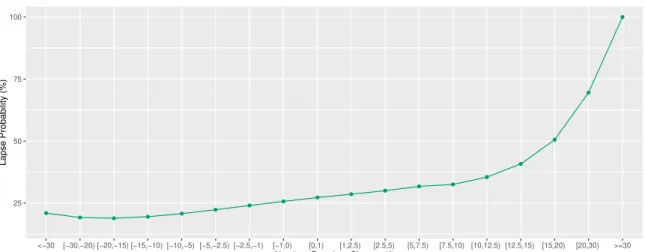
25 50 75 100

<−30 [−30,−20) [−20,−15) [−15,−10) [−10,−5) [−5,−2.5) [−2.5,−1) [−1,0) [0,1) [1,2.5) [2.5,5) [5,7.5) [7.5,10) [10,12.5) [12.5,15) [15,20) [20,30) >=30

Absolute Premium Change (€)

Lapse Probability (%)

Lapse Probability per Premium Change Other variables set to base level

Figure 4.2: Effect of premium change on cancellations

Higher increases in premium lead to higher cancellation probabilities, as expected.

However, the lapse probability flattens off where premium decreases are around AC15

and then increases slightly. Similar effects were observed by Blandet al.(1997) and by

Garraio (2015), with Murphyet al.(2000) stating that this effect is typical of elasticity

curves. Since large decreases are often already anticipated by the customers that receive

them (e.g. by moving to anotherbonus-malus level), one possible justification for this

effect is that those clients feel that the decrease isn’t large enough (Garraio, 2015).

Another possibility is that clients may not understand why they paid so much in the

previous term, compared to what the new premium is, triggering them to look for

alternative prices elsewhere (Murphyet al., 2000; Guven and McPhail, 2013).

Since our final model has interaction terms between the absolute premium change

and three other factors, each client’s estimated price elasticity curve won’t necessarily

have the same shape as the one shown in Figure 4.2. This way, more insights are

gained regarding how the sensitivity to premium variations varies between different

subpopulations of the portfolio.

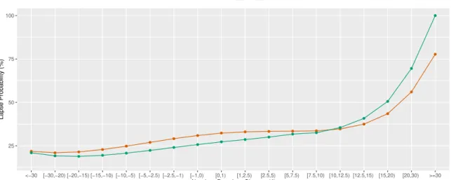
Figure 4.3 shows the same as the previous figure, only this time distinguishing

between clients with and without own damage coverage.

The first interaction effect with the premium change is clear, as policyholders with

additional covers pay higher premiums and are therefore less sensitive to large absolute

variations. Additionally, clients with this coverage tend to care more about the product

(35)

25 50 75 100

<−30 [−30,−20) [−20,−15) [−15,−10) [−10,−5) [−5,−2.5) [−2.5,−1) [−1,0) [0,1) [1,2.5) [2.5,5) [5,7.5) [7.5,10) [10,12.5) [12.5,15) [15,20) [20,30) >=30

Own damage No Yes

Figure 4.3: Effect of own damage on cancellations

also help explain this effect.

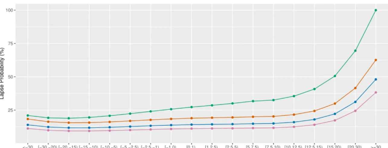
Similarly, claimants are less sensitive to large increases in premium, as can be seen

in Figure 4.4. This effect is in agreement with the results of Guelman and Guill´en

(2014) and occurs since those customers already expect some premium increase. We

remark that the number of clients with claims and who had premium decreases larger

thanAC15 is very small (approximately 2% of the dataset), making it harder to retrieve

any conclusion from the estimated increase in price sensitivity for these clients.

25 50 75 100

<−30 [−30,−20) [−20,−15) [−15,−10) [−10,−5) [−5,−2.5) [−2.5,−1) [−1,0) [0,1) [1,2.5) [2.5,5) [5,7.5) [7.5,10) [10,12.5) [12.5,15) [15,20) [20,30) >=30

Claim No Yes

Figure 4.4: Effect of claims on cancellations

Regarding the payment frequency, Figure 4.5 confirms our expectations that the

(36)

25 50 75 100

<−30 [−30,−20) [−20,−15) [−15,−10) [−10,−5) [−5,−2.5) [−2.5,−1) [−1,0) [0,1) [1,2.5) [2.5,5) [5,7.5) [7.5,10) [10,12.5) [12.5,15) [15,20) [20,30) >=30

Payment Frequency Annual Semi−annual Quarterly Monthly

Figure 4.5: Effect of payment frequency on cancellations

since they receive the full price increase at once.

We emphasise that the bonus-malus discount and the number of other

cancella-tions, besides exhibiting their expected effects, have a noticeable impact on the lapse

probability. Also, customers with several policies in the company have lower

cancel-lation probabilities, showing that clients care about keeping their different insurance

products in one company (Barone and Bella, 2004).

The effects of the different tariffs on the response reinforce the notion that, when

designing new tariffs or products, the long term impact on retention should be taken

into account, and not just the short term impact on new business.

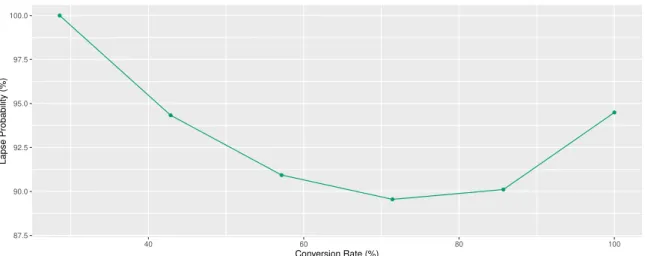
We recall that we estimated the conversion rate per time of year and customer

profile, with Figure 4.6 showing the lapse probability per conversion rate. Since higher

conversion rates are associated with competitive premiums, we expected the lapse

probability to decrease as the estimated conversion rate increased. While this effect

can be observed at first, we see the opposite effect occurring for very high conversion

rates.

As mentioned in subsection 2.2.1, conversion rates are a measure of

competitive-ness on new busicompetitive-ness, not of renewal competitivecompetitive-ness. We thus believe that policy

cannibalisations (clients cancelling their old policy to make a new one) and clients

that tend to shift companies very often are what’s causing lapse rates to increase for

high conversion profiles.

(37)

87.5 90.0 92.5 95.0 97.5 100.0

40 60 80 100

Conversion Rate (%)

Lapse Probability per Conversion Rate Other variables set to base level

Figure 4.6: Lapse probability per conversion rate

as clients who change their policy and consequently see their premium rise are more

prone to cancelling it during the renewal period. As mentioned in subsection 2.2.3, one

possible reason for this may be that clients only become fully aware of the impact on

the premium when the new policy term begins.

As for the district where the customer lives, the final aggregation resulted in groups

with districts which are, in several cases, very far apart from each other. We believe

that this result may be linked to how the level of competition in Motor insurance

differs from one to district to another.

Overall, the effects of the remaining covariates matched our expectations and the

(38)

Chapter 5 Obtaining binary predictions

Our two main objectives for this work were creating a model for the probability of

policy cancellation and, at the same time, gaining insights on how different factors

influence renewals. As a consequence, if a covariate wasn’t significant and/or didn’t

make sense it was promptly removed from the model, even if keeping it would have

increased the model’s predictive ability (as measured by AUC).

Still, it’s clear that obtaining predictions on which clients will cancel their policies

would be advantageous for the insurer, as it could, for instance, help the company

select which clients should be the target of retention measures during the renewal

period.

In this chapter we analyse the model’s predictive ability and study different

thresh-old optimisation criteria, to obtain the best threshthresh-old based on overall performance,

using the binary classification measures discussed in section 3.3.

5.1 Evaluating predictive ability

The ROC curves resulting from the application of the model on the training and

test sets are shown in Figure 5.1. The value of the AUC on the training set is 0.702,

indicating fair discriminatory capacity (Kleinbaum and Klein, 2010). As expected,

when applying the model on the test set the AUC decreases, to 0.678. It’s a small

decrease nevertheless, indicating no strong sign of overfitting and leading us to conclude

that model’s predictive ability translates well into unseen data.

(39)

5.1. Evaluating predictive ability

0.0 0.2 0.4 0.6 0.8 1.0

0.0 0.2 0.4 0.6 0.8 1.0 1−Specificity Sensitivity AUC: 0.70 Training Training set

0.0 0.2 0.4 0.6 0.8 1.0

0.0 0.2 0.4 0.6 0.8 1.0 1−Specificity Sensitivity AUC: 0.68 Test Test set

Figure 5.1: ROC curves (both datasets)

discrimination, this histogram would have almost all renewals on the left side, with

low probability, and almost all lapses on the right side with high probability, showing

clear separation between classes. In that case it would be possible to find a threshold

that could easily discriminate between both classes. However, what we observe is that

while renewals are gathered on the left side of the graph, lapses are spread out over

a large range of probabilities. This is a consequence of the severe class imbalance in

our dataset (the lapse rate is lower than 15%). As most clients renew, the model can

easily achieve high specificity, but predicting cancellations (our event of interest) is

much harder.

Lapse Probability

Number of Obser

vations 0 5000 15000 25000 35000

0.0 0.2 0.4 0.6 0.8 1.0

Lapses

Renewals

Histogram

(40)

5.2. Threshold optimisation

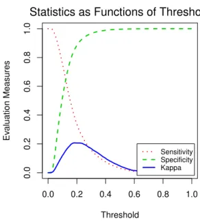
Figure 5.3 shows sensitivity, specificity and kappa on the training set as functions of

threshold. As expected, specificity has a sharp increase, due to the renewals having been

assigned mostly small probabilities. On the other hand, sensitivity decreases quickly

- to capture most of the lapses the model yields a large number of false positives.

Kappa, which evaluates the model’s discriminatory ability overall, is consequently low

for most of the threshold range, barely going above 0.2 at its maximum.

0.0 0.2 0.4 0.6 0.8 1.0

0.0

0.2

0.4

0.6

0.8

1.0

Threshold

Ev

aluation Measures

Sensitivity Specificity Kappa Statistics as Functions of Threshold

Figure 5.3: Sensitivity, specificity and kappa (training set)

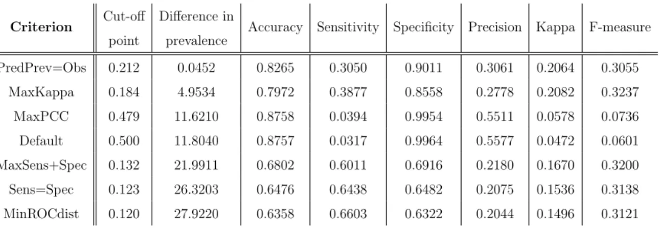
5.2 Threshold optimisation

Since the model displays a reasonable predictive capacity, we now need to define a

threshold to obtain actual lapse predictions from the model. Several threshold

optimi-sation criteria exist, and in our work we consider 7 of such criteria which have been

previously analysed by Freeman and Moisen (2008a).1 _{Besides the evaluation}

mea-sures discussed in section 3.3, we also look at the difference between the observed and

predicted prevalence (lapse rate) given by each threshold. The different criteria are

presented below in bold.

Usually, the thresholds should be determined using a set other than the training

or test sets, especially when dealing with small samples. This is to avoid an overly

1

Freeman and Moisen (2008a) studied additional criteria, such as criteria where the sensitivity or

(41)

optimistic assessment of the model’s quality and to keep the test set completely

in-dependent from the model building process (Kuhn and Johnson, 2013). In this work

however, the training set was chosen to examine the criteria (since we have a large

enough sample), making use of the R package ‘PresenceAbsence’ (Freeman and Moisen,

2008b). The results are shown in Table 5.1 (see section C.2 for the R output).

Criterion Cut-off

point

Difference in

prevalence Accuracy Sensitivity Specificity Precision Kappa F-measure

PredPrev=Obs 0.212 0.0452 0.8265 0.3050 0.9011 0.3061 0.2064 0.3055

MaxKappa 0.184 4.9534 0.7972 0.3877 0.8558 0.2778 0.2082 0.3237

MaxPCC 0.479 11.6210 0.8758 0.0394 0.9954 0.5511 0.0578 0.0736

Default 0.500 11.8040 0.8757 0.0317 0.9964 0.5577 0.0472 0.0601

MaxSens+Spec 0.132 21.9911 0.6802 0.6011 0.6916 0.2180 0.1670 0.3200

Sens=Spec 0.123 26.3203 0.6476 0.6438 0.6482 0.2075 0.1536 0.3138

MinROCdist 0.120 27.9220 0.6358 0.6603 0.6322 0.2044 0.1496 0.3121

Table 5.1: Threshold optimisation results (training set)

The Default criterion, simply consisting of a cut-off point of 0.5, and the Max-PCCcriterion, maximising accuracy2_{, give similar results. While accuracy is very high}

in both cases, due to the class imbalance this is done by “focusing” on renewals, as

they’re much more prevalent, resulting in exceptionally high specificity and extremely

low sensitivity. Precision is higher than for other criteria, due to only the policies

with very high probabilities actually being predicted as lapses. This “unbalance” in

the statistics is reflected by very low values of kappa and F-measure, indicating poor

discriminatory performance.

Sens=Spec finds the threshold where sensitivity equals specificity, while Max-Sens+Spec maximises the sum of the two. As mentioned in subsection 3.3.1, the point (0,1) in ROC space implies perfect discrimination. TheMinROCdist criterion therefore finds the threshold minimising the Euclidian distance to that point. While

precision is now lower for these three criteria, sensitivity is much higher than

be-fore, which is reflected by the increase in F-measure. Still, the predicted and observed

prevalence are too far apart and while kappa is higher than before it’s still possible to

improve it.

2

Percent Correctly Classified (PCC) is the denomination given by Freeman and Moisen (2008a)

(42)

PredPrev=Obs finds the threshold where the predicted prevalence equals the observed one andMaxKappa maximises kappa. They result in the two highest values of kappa and the two lowest differences between observed and predicted prevalence,

with Freeman and Moisen (2008a) observing similar results in their work.MaxKappa

however resulted in a better balance between sensitivity and precision, as given by

F-measure.

If the company wishes to use this model for prediction, we therefore recommend

applying a threshold of 0.184 (MaxKappa), based on overall performance.

The test set has an even lower prevalence than the training set (by 1.88 pp). Besides

the expected decrease in performance when moving to new data, this higher proportion

of renewals means that all the previously computed thresholds lead to lower sensitivity,

precision, kappa and F-measure (when compared with the training set). Once again,

see section C.2 for the R output.

Regarding our chosen threshold of 0.184, the results from the test set are presented

in Table 5.2. Despite the predicted and observed prevalence now being much closer

than when we used it on the training set, there is an obvious decrease in overall

performance, as seen by the low values of kappa and F-measure.

Criterion Cut-off

point

Difference in

prevalence Accuracy Sensitivity Specificity Precision Kappa F-measure

MaxKappa 0.184 0.0515 0.8393 0.2469 0.9098 0.2457 0.1563 0.2463

Table 5.2: Application of the chosen threshold (test set)

We stress that prediction wasn’t our main goal and that class imbalance in the

data notably leads to worse model performance. We believe however that using

sim-ply remedies for class imbalance, such as basic resample methods to construct more

balanced datasets, could lead to significant improvements in model performance, if

prediction is the ultimate goal. For more on dealing with the class imbalance problem

in lapse prediction, including different resampling methods and other models more