Approximate solutions of large amplitude vibration of a string

(1)

Approximate solutions of large amplitude vibration of a string

Abstract

In the present study, the response of a flexible string with large amplitude transverse vibration is studied utilizing amplitude-frequency formulation, improved amplitude-frequency formulation and max-min approach. In or-der to verify the accuracy of these approaches, obtained results are com-pared with other methods such as variational approach method, variational iteration method, coupling Newton’s method with the harmonic balance method and Hamiltonian approach. It has been found that for this problem, while amplitude-frequency formulation and max-min approach give the same results, improved amplitude frequency formulation is not an appro-priate choice.

Keywords

nonlinear vibration, string, amplitude-frequency formulation, improved am-plitude-frequency formulation and max-min approach.

1 INTRODUCTION

Study of nonlinear vibration of strings with large amplitude has attracted the attention of many researches in the fields of physics and engineering. For instance, long cables used in cranes, ships and bridges might expose to forces that causes large amplitude vibrations (Omran et al., 2013). The nonlinear partial differential equation for transverse vibrations of a flexible string under constant tension is presented in equation (1)(Coulson and Jeffrey, 1997).

2 2

2 2 2

2

[1 ( ) ]

2

u

c

x

t



_{ }



(1)

where

c

2



 

0 0, with



0the tension and



0the mass per unit length. The boundary conditions for the string of

length L, vibrating between two fixed end-points are presented in equation (2).

(0, )

( , ) 0

u t



u L t



(2)

By considering the transverse vibration as

u x t V t

( , )

( )sin(

x

)

L





, substituting it into equation (1) and aver-aging over the string length L, an ordinary second-order differential equation (3) is derived as presented in equa-tions (3) - (6)(Gottlieb, 1990).

2

2 4

2

0

1

2

8 d S

S

dt









(3)

where

( )

S t

V t

L





(4)

Rayehe Karimi Mahabadia Mitra Danesh Pazhoohb

*

a_{Department of Mechanical Engineering,}

AmirKabir University of Technology (Tehran Polytechnic), Post Box: 15875-4413, Tehran, Iran Author email: rayehe_karimi@aut.ac.ir

b_{Department of Mechanical Engineering,}

AmirKabir University of Technology (Tehran Polytechnic), Post Box: 15875-4413, Tehran, Iran Author email: daneshm@aut.ac.ir

*Corresponding author

http://dx.doi.org/10.1590/1679-78254122

Received: June 15, 2017

(2)

2

( )

c

L







(5)

with initial conditions

(0)

S



a

,

dS

(0) 0

dt



(6)

Many researches have been conducted to solve equation (3) with different methods such as variational ap-proach method, variational iteration method, coupling Newton’s method with the harmonic balance method and Hamiltonian approach. In the present study, this equation is solved using amplitude-frequency formulation, im-proved amplitude-frequency formulation and max-min approach. Furthermore, obtained results are compared with that of the mentioned methods.

2 METHODOLOGY

2.1 Amplitude-frequency formulation (AFF)

To illustrate this approach, a generalized nonlinear oscillator is considered as presented in equation (7)

( ) 0

u

 

f u



_,

u

₍₀₎



A

_,

u



_{(0) 0}



₍₇₎

Used Trial functions are presented in equation (8) and (9).

1

( )

cos( )

1

u t



A



t

(8)

2

( )

cos( )

2

u t



A



t

(9)

The residuals are as shown in equations (10) and (11).

2

1

( )

1

cos( )

1

( cos( ))

1

R t



 

A



t



f A



t

(10)

2

( )

2

cos( )

2

( cos( ))

2

R



t

 

A



t



f A



t

(11)

The original frequency-amplitude formulation is presented in equation (12).

2 2

2 1 2 2 1 2 1

R

R R







(12)

To find the frequency, He (2008a) used equation (13), Geng and Cai (2007) used another location point which is indicated in equation (14). By substituting



from these equations into

u t

( )



A

cos( )



t

and considering

1 2

cos( ) cos( )



t





t



k

_{, the frequency is obtained.}

2 2

2 1 2 2 2 1 1

2 1

(

0)

(

0)

R

t

R

t

R R





 





(13)

2 2

2 1 2 2 2 1 1

2 1

(

/ 3)

(

/ 3)

R

t

R

t

R R



















(14)

To solve equation (3),

u t

1

( )



A

cos

t

and

u t

2

( )



A

cos2

t

are selected as trial functions. Substituting these

functions into equation (3), the residuals are computed as follows,

1

cos( )

2

_{cos ( )}

2 4

_{cos ( )}

4

1

2

8 R

a

t a

t

a

t

a

t



 



(3)

2

4 cos(2 )

cos(2 )

2

_{cos (2 )}

2 4

_{cos (2 )}

4

1

2

8 R

a

t a

t

a

t

a

t



 



(16)

Substituting equations (15) and (16) in equation (12) and considering

cos( ) cos(2 )

t



t



k

yields equation (17).

2 2 4 4 2 2 4 4

2

2 2 4 4

4 4(

)

1

2

8

2

8

4 ₁

2

8 ak

ak

a k

ak ak









 









_

(17)

Parameter k can be drawn by substituting the natural frequency from equation (17) into the integral equation (18) and assuming

u t

( )



a

cos( )



t

.

2 4

2 2 4 4

0

(

cos

)cos

0

1

2

8

T

a

t a

t

tdt

a

t a

t













(18)

2.2 Improved amplitude-frequency formulation (IAFF)

The accuracy of AFF depends upon the location choice. He (2008b) suggested the method of weighted residual to overcome this shortcoming. A generalized nonlinear oscillator is considered as presened in equation (19).

( ) 0

u

 

f u



,

u

(0)



A

,

u



(0) 0



(19)

Respectively, solutions of the following linear oscillator equations are considered as two trial functions

1

( )

cos

u t



A

t

and

u t

2

( )



A

cos



t

which are respectively represented in equations (20) and (21). 2

1

0 u

 



u



2 1

1 



(20)

2 2

0 u

 



u



2 2 2







(21)

where



is assumed to be the frequency of the nonlinear oscillator in equation (19). The residuals are presented in equations (22) and (23).

1

( )

cos

( cos )

R t

 

t f A



t

(22)

2

( )

cos

( cos )

R



t

 



t f A





t

(23)

In this approach, to overcome the shortcomings, two new residuals are defined as

R

~1 and ~

2

R

as presented in equations (24) and (25).

1/4 ~

1 1

1 0 1

4

T

_{( )cos(}

2 ₎

R

R t

t dt

T







(24)

2/4 ~

2 2

2 0 2

4

T

_{( )cos(}

2 ₎

R

R t

t dt

T







(25)

(4)

~ ~

2 2

2 1 2 2 1 ~ ~

2 1

R

R R







(26)

To solve equation (3) by this method, trial functions are considered as

u t

1

( )



A

cos

t

and

u t

1

( )



A

cos



t

.

Substituting these functions into equation (3), the residuals are computed as presented in equation equation (27) to (30).

1

cos

2

_cos

2 4

_cos

4

1

2

8 R

a

t a

t

a

t a

t



 



(27)

~

2 1

₂

4

₀ 1

cos

R



_





R

tdt

(28)

2

cos

2

_cos

2 4

_cos

4

1

2

8 R

a

t a

t

a

t a

t





 



(29)

~

2

4 ₂

₀ 2

cos

R





R



tdt





_

(30)

By changing variable to

s





t

, the residual

R

~2can be rewritten as presented in equation (31). ~

2

₀ 2

cos( )

R



R

s ds







(31)

Frequency can be obtained by substituting

R

~1and ~

2

R

into equation (26).

2.3 Max-min Approach (MMA)

In this approach, after finding the maximal and minimal solution thresholds, an approximate solution of the nonlinear equation is deduced using He-Chengtian’s interpolation (He, 2008c). For instance, a generalized nonlin-ear oscillator is considered in the form of equation (32),

( ) 0

u u f u







u

(0)



A

u



_{(0) 0}



(32)

where

f u

( )

is a non-negative function of u. The trial function is considered to be

u t

( )



A

cos( )



t

, where



is the frequency. Considering the linear oscillator, equation (33),

min

0 u u f







,

u

(0)



A

,

u



(0) 0



(33)

where

f

minis the minimum value of the function

f u

( )

, the square of frequency in equation (32) is never less than

that of equation (33) with the solution in the form of

u t

1

( )



A

cos(

f t

min

)

. In addition, the square of frequency

never outdoes that of the oscillator in equation (34) which has the solution in the form of

u t

1

( )



A

cos(

f t

max

)

.

max

0 u u f







,

u

(0)



A

,

u



(0) 0



(34)

where

f

maxis the maximum value of the function

f u

( )

. Hence, equation (35) can be concluded. (Bayat et al., 2012) 2

min max

f







f

(35)

(5)

2

mf

min

nf

max

m n







(36)

where

m

and

n

are weighting factors. By defining

k n m



/

, the previous equation can be rewritten as equation (37).

2 min max

1 f

kf

k







(37)

By substituting the frequency from equation (37) into the assumed solution of equation (34), the residual is obtained as equation (38).

2

_{cos( ) ( cos( )). ( cos( ))}

R

 



A



t



A



t f A



t

(38)

Solving equation (39), k is obtained as indicated in equation (40).

2 min max 0

cos

0

1 f

kf

R

tdt

k

 

_







(39) max min 2 0

1 cos . ( cos )

f

k

A



_{x f A}

_{x dx}











(40)

Substituting k from equation (40) into equation (37), frequency can be obtained (Bayat et al., 2012).

To apply this method for the nonlinear partial differential equation for transverse vibrations of a flexible string, equation (1) is rewritten in the form of equation (41).

( ) 0

u u f u







(41)

where

( )

₂ ₄

1

2

8 u

f u

u







. The trial function to solve equation (41) is considered as

u t

( )



A

cos



t

. Frequency

is computed utilizing equation (37), in which

f

min and

f

maxare substituted from equations (42) and (43).

min 2 4

1

2

8 f

a







(42)

max

f





₍₄₃₎

Substituting equations (42) and (43) into equation (37), square of the frequency is obtained as indicated in equation (44).

2 2 4 4

2

1

2

8

1 k

a k

k



_









(44)

Substituting equation (44) into the equation (41), the residual is presented in equation (45).

2

2 2 4 4

cos

1

2

8 R a

t a

t

a

t a

t









(6)

By using equation (46) and equation (44), the frequency can be attained. The obtained results are compared in the next section.

2 4

2 2 4 4

0

(

cos

) cos

0

1

2

8

T

a

t a

t

tdt

a

t a

t















(46)

3 Results and discussion

3.1 Free vibration response of the cable

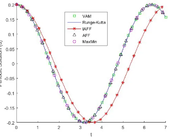
The response of the cable under free vibration is compared by different methods, including VAM, Fourth order Runge-Kutta, IAFF, AFF and MaxMin, for different amplitudes in Figure 1 to Figure 5.

(7)

Figure 2: Response comparison for

a



0.2

and





1

.

(8)

Figure 4: Response comparison for

a



5

and





1

.

(9)

Obtained solutions using AFF, IAFF, MMA and Runge-Kutta are compared to the results of variational Iteration Method (VIM) (Taghipour et al., 2014), Hamiltonian Approach (HA) (Taghipour et al., 2014) and Variational ap-proach method (VAM) which is reproduced using the derived equations in (Omran et al., 2013) in Table 1 and Table 2.

Table 1: Response comparison when

t



0.5( )

s

and





1

.

a _{(Taghipour et al., 2014) (Taghipour et al., 2014)}VIM HA VAM (Omran et al., 2013) IAFF AFF MMA Runge-Kutta 3 2.7467 3.0299 2.9605 2.9608 2.9501 2.9501 2.9759 4 3.8690 4.0171 3.9783 3.9743 3.9673 3.9673 3.9878 5 4.9267 5.0102 4.9874 4.9823 4.9775 4.9775 4.9931 10 9.9691 10.0016 9.9981 9.9951 9.9938 9.9938 9.9990

Table 2: Response comparison when

t



1( )

s

and





2

.

a _{(Taghipour et al., 2014) (Taghipour et al., 2014)}VIM HA VAM (Omran et al., 2013) IAFF AFF MMA Runge-Kutta 3 2.6120 3.2420 2.6891 1.6209 2.6089 2.6089 2.8034 4 3.4277 4.1377 3.8278 2.1612 3.7412 3.7412 3.9014 5 4.7012 5.0816 4.8993 2.7015 4.8210 4.8210 4.9452 10 9.5103 10.0130 9.9849 5.4030 9.9503 9.9503 9.9923

Comparing the results in tables 1 and 2, the computed response of the cable under the large amplitude vibra-tion using VAM, AFF and MMA are near eachother, while those of the IAFF is far apart from other methods. Moreo-ver, the obtained results by MMA and AFF are the same for this problem.

3.2 Period parameter

The obtained period parameter



T

from AFF, IAFF and MMA are compared to that of VAM (Omran et al., 2013), second-order analytical approximation constructed by harmonic balance method (Gottlieb, 1990), First-order, second-order and third-order analytical approximation developed by coupling Newton’s method with the harmonic balance method (NHB) (Lai et al., 2008) and the exact solution (Lai et al., 2008).

Table 3: Comparison of the period parameter T_.

a



T

exact



T

HB2



T

1



T

2



T

3

(Lai et al., 2008) (Gottlieb, 1990) (Lai et al., 2008) (Lai et al., 2008) (Lai et al., 2008)

0.1 6.294977 6.294980 6.294977 6.294977 6.294977

0.2 6.33047 6.33052 6.33047 6.33047 6.33047 0.5 6.58377 6.58576 6.58377 6.58379 6.58379

5 42.173 48.345 42.173 41.875 41.918

10 152.9 179.9 152.9 149.4 148.8

a



T

VAM



T

_IAFF



T

_AFF



T

_MMA

(Omran et al., 2013)

0.1 6.294975 7.103118 6.294975 6.294975

0.2 6.33047 7.14314 6.33044 6.33044

0.5 6.58372 7.42763 6.58257 6.58257

5 44.2076 37.3552 33.1052 33.1052

(10)

Comparing the results in table 3, one can conclude that for small values of a, obtained results by MMA and AFF is in agreement with the exact solution, and by increasing the value of a, the results deviate from the exact solution. Moreover, utilizing IAFF for this problem is not appropriate since its error is more than other mentioned methods.

4 CONCLUSION

In this paper, AFF, IAFF and MMA are employed to derive the analytical approximate solution for large ampli-tude nonlinear vibration of a string. The obtained response from these methods were compared to other methods such as VAM, VIM, HA and HB. It is shown that the obtained response from MMA and AFF are the same for this problem. On the other hand, IAFF is not appropriate method for this problem since it is not accurate enough in comparison to other mentioned methods.

References

Bayat, M.; Pakar, I.; Domairry, G.; “Recent developments of some asymptotic methods and their applications for nonlinear vibration equations in engineering problems: A review”, Latin American Journal of Solids and Structures, 9(2) 1-93, 2012.

Coulson, C.A.; Jeffrey, A.; Waves, 2nd edition, London: Longman, 1997.

Geng, L.; Cai, X.C. “He’s frequency formulation for nonlinear oscillators”, European Journal of Physics, 61(8) 923-931,2007.

Gottlieb, H.P.W.; “Non-linear vibration of a constant-tension string”, Journal of sound and vibration, 143(3) 455-460, 1990.

He, J.H.; “An elementary introduction to recently developed asymptotic methods and nanomechanics in textile en-gineering”, International Journal of Modern Physics B, 22(1) 3487-3578, 2008a.

He, J.H.; “Comment on He's frequency formulation for nonlinear oscillators”, European Journal of Physics, 29, 19-22, 2008b.

He, J.H.; “Max-min approach to nonlinear oscillators”, international Journal of Nonlinear Sciences and Numerical Simulation, 9(2) 207-210, 2008c.

Lai, S.K.; Xiang, Y.; Lim, C.W.; He, X.F.; Zeng, Q.C.; “Higher-order approximate solutions for nonlinear vibration of a constant-tension string”, Journal of Sound and Vibration, 317(3-5) 440-448, 2008.

Omran, M.P.; Amani, A.; Lemu, H.G.; “Analytical approximation of nonlinear vibration of string with large ampli-tudes”, Journal of Mechanical Science and Technology, 27(4) 981-986, 2013.