Vectors
Aluizio Arcela
Department of Computer Science University of Brasilia Campus Universitário, Asa Norte
Phone: +55 (61) 33072705 Zip 70910-900 - Brasilia - DF - BRAZIL
Received 07 January 2008; accepted 04 July 2008
Abstract
A pitch model is proposed which is supported by a vec-tor representation of tones. First, an algorithm capable of performing the vector addition of the spectral components of two-tone harmonic complexes is introduced which ini-tially converts the amplitude, frequency, and phase (AFP) parameters into coordinates of the here introduced quo-tient, distance in octaves, and loudness (QOL) tone space. As QOL is isomorphic to the hue, saturation, and value (HSV) color space, a transformation from QOL to the red, green, and blue (RGB) vector space can be formulated so that the vector addition of two pure tones is conceived by analogy with color mixing operations. Since the QOL to RGB transformation is invertible, the resulting RGB vector sum can be transformed back to QOL. Then, by converting QOL coordinates back to AFP parameters, a tone is found whose frequency supposedly corresponds to the pitch evoked by the original two-tone complex. As for complexes having more than two components, the al-gorithm is to be sequentially applied to pairs of vectors in such a way that initially the first two vector tones are added together, then the resulting vector is added to the third vector tone, and so on.
Keywords: pitch computation, vector representation of tones, two-tone complexes, missing undamental.
1. I
NTRODUCTIONSeebeck [21] proposed a relationship between pitch and periodicity after having observed that the wave-form’s repetition period could be perceived as pitch even if there is no spectral component at the corresponding
frequency—a consideration which gave rise to the con-cept of “missing fundamental”. Later on, a dispute began between Seebeck and Ohm [16], who believed that to a perceived pitch there corresponds the frequency of a non-null spectral component. Some years later, von Helmholtz [31] presented arguments in favor of Ohm’s view, when he further conjectured about a possible analogy between the phenomena of mixed colors and those of compound musical tones. Incidentally, this latter hypothesis is taken as the starting point of the present study which is con-cerned with applying the mathematics of colors to pitch computation.
This paper assumes that three-dimensional vectors are an appropriate representation of tones since they have means of adding them in a convenient way. Indeed, the addition of pure tones as vectors does not yield a “com-plex” [10], such as occurs in the addition of pure tones as sinusoids, but it just yields a single pure tone. Fur-thermore, taking into account that a complex is always characterized by one definite pitch [19], it is hypothesized here that the addition of tones as vectors can find a result-ing tone whose frequency corresponds to such definite pitch. This tone is called here the vector addition tone, while its frequency is referred to as the computed pitch.
equi-librium theorem—from which a loudness scale is derived for pure tones. Finally, it describes how to find a measure of the symmetry of the second-derivative’s zero-crossing pattern, which acts as a magnitude coefficient in the vec-tor addition operation.
Section 3 introduces the vector representation of tones in two subsections. In the first one, it defines the quotient, distance in octaves, and loudness (QOL) space for rep-resenting tones in a three-dimensional system. Any pure tone expressed in amplitude, frequency, and phase (AFP) parameters can be represented in the QOL space. In the second subsection, by taking into account that the QOL’s mathematical structure is isomorphic to that of the hue, saturation, and value (HSV) color space [30], it shows that QOL tones can be converted to red, green, and blue (RGB) colors, so that any pure tone can be expressed as a RGB vector.
Section 4 details how to compute the overall vector addition tone for harmonic complexes by first describing the algorithm for the vector addition of two tones. This also includes the inverse transformations which are to be applied initially from RGB back to QOL, and then from QOL back to AFP. Next, it shows how the final pitch is computed for harmonic complexes having more than two components by adding vector pairs across the com-ponents.
Section 5 first shows how pitch is related to fre-quency ratios in two-tone harmonic complexes, a descrip-tion based on the geometric properties of the vector repre-sentation of tones. Subsequently, it describes how phase relationships affect the pitch of these complexes.
Section 6 ends the paper with a discussion on the con-ditions necessary for the pitch of a complex being equal to the frequency (F0) of the fundamental, along with the pitch computation of ten selected complexes having more than two components. They are presented in a sequence which intends to illustrate the main points of the men-tioned conditions, being the first three complexes taken from the literature so as to compare the results found in this study with those of some important pitch models (e.g., [5, 6, 8, 17, 18, 29, 32]) either from the “temporal” view, which is based on the “autocorrelation” hypothesis raised by Licklider [13], or from the “pattern matching” models which was first described by de Boer [6]. The re-sults found with vector addition tones show that the pitch of harmonic complexes corresponds to the frequency of the fundamental only in some special cases.
2. K
EYP
ROPERTIES OFT
WO-T
ONEH
ARMONICC
OMPLEXESSome concepts introduced in this paper are derived from two-tone harmonic complexes. In this way, a
math-ematical description of these complexes is given be-low by using a terminology as close as possible to that found in the literature related to such class of complexes [7, 10, 11, 25]. A few terms are introduced, however, as a consequence of considering other aspects of two-tone complexes, as the equilibrium (Section 2.2) and the sym-metry of the second derivative with respect to time (Sec-tion 2.3).
The lower componentx(t)and the upper component
y(t)of a two-tone harmonic complex are according to
x(t) =axsin (2πfxt+px) (1)
and
y(t) =aysin (2πfyt+py), (2)
whereaxanday are amplitudes;fxandfy are frequen-cies; and px andpy are phase angles (in radians; when expressed in degrees, they are represented as [px] and
[py]). The addition of these components together defines the class of two-tone harmonic complexesc(t), orm:n -complexes for short, that is,
c(t) =x(t) +y(t). (3)
t t + τ c
x(t ): Lower component
( c ) ( b ) ( a )
y(t ): Upper component
c(t ): Two-tone complex
time
Figure 1. Sinusoid addition of lower and upper components of a two-tone harmonic complex.
There are three properties ofm:n-complexes which are relevant to the present theory, as described below in Sec-tions 2.1-2.3.
2.1. THE PERIOD OFm:n-COMPLEXES
The first relevant property of am:n-complex is that its period is calculable. That is to say, since the ratio between its component frequencies can be written as
fx fy =
m
n, (4)
where m and n are integers such that m ≤ n and
one periodτcof am:n-complex comprisesmperiods of
x(t)againstnperiods ofy(t), that is,
τc= m fx =
n
fy. (5)
Therefore, to find the period of a m:n-complex from Equation (5), it is first necessary to find one of the num-bersmorn, which can be done by means of the equations
m= num ·
F µ
fx fy
¶¸
(6)
and
n= den ·
F µfx
fy ¶¸
, (7)
whereFis a method for converting a decimal number to a common fraction reduced to lowest terms, that is, the methodFgives two integers, being the first one collected by the methodnumwhile the second one is collected by the methodden. These two numbers are referred to here as reduced harmonic numbers.
As studied in Sections 2.2 and 2.3, the focus here is that the period τc is a length of time along which the waveform of am:n-complex (1) has a well-defined num-ber of peaks, and (2) the symmetry of the zero-crossing pattern of its second derivative with respect to time af-fects the amplitude of the vector addition tone, as studied in Section 4.
2.2. THE EQUILIBRIUM THEOREM
The second relevant property is related to the num-ber of maxima am:n-complex has within one periodτc. Since this number is exclusively either mor n, am:n -complex may be said to have two states: thelow state, when there aremmaxima within the periodτc, and the high state, when there arenmaxima. In this way, there is a border separating the low from the high state, which is referred to here as theequilibriumof them:n-complex.
One way of counting the number of maxima is by means of the waveform inflection points, for any maxi-mum occurs in a curve segment having a down concavity. Since the inflection points, that is, the points where the concavity changes from up to down, occur at values oft
where the second derivative ofc(t)with respect to time is null, this second derivative must be taken and then its zero crossings must be found so as to determine the number of times the concavity of the complex’s waveform changes from up to down.
All possible waveforms for am:n-complex at a given phase relationship can be obtained by holdingaxconstant while allowing ay to vary from a small value up to be equal toax, as shown in Figure 2 for one period of a4: 5 -complex with phasespx = py = π/2. The waveforms in the upper half-surface are in the low state, all of them
having four maxima, that is,mpeaks, whereas the wave-forms in the bottom half-surface are in the high state, all of them having five maxima, that is,npeaks. At the bor-der between these states, the waveform is in equilibrium, as shown by the thick waveform drawing.
1 2 3 4 5 1
1 2 3 4 1
t[sec] t + τ c
Low state
High state
peak number
Figure 2. The two possible states in a full periodτcof a4: 5-complex
along with the equilibrium waveform (the white line) which is the boundary between the regions of low and high states.
Phase relationships between px andpy do not cause changes of state. Although they can modify the position of the inflection points, they cannot change the number of them. The state can only be changed by amplitude changes, for there is a well-defined amplitude propor-tionax/ay associated to the equilibrium of everym:n -complex. Such proportion is given by a theorem [1], which is stated as follows.
Theorem 1 (Equilibrium theorem)Am:n-complex is in equilibrium if
ax ay =
³n
m ´2
. (8)
Proof.Lettµbe a instant such that0≤tµ < τcat which the lower tonex(t)is at a maximum, i.e.,x(tµ) =ax, as shown in Figure 1. In terms of periodsτxofx(t), it can be expressed as
tµ=kτx+ ∆t, (9)
wherek is the number of full periodsτx between0 and
tµ, i.e., k = int(tµ, τx); and ∆t is the amount of time separating the end of theseksuccessive periods fromtµ, i.e., ∆t = mod(tµ, τx). Therefore, according to Equa-tions (1) and (5), the phasepxneeded for the occurrence of a maximum ofx(t)attµis such that
m µ2πtµ
τc 
+px= (4k+ 1)π
2. (10)
x(t )
y(t)
ax
- ay
kτx ∆t
τ
x 2τx
t µ
0 time τ c
Figure 3. The lower and upper componentsx(t)andy(t)can be displaced with respect to one another, so that a maximum of one of the
sinusoids occurs at the same instant a minimum of the other also occurs. More precisely, to every phasepxof the lower tone, there is a
phasepyof the upper tone where at a given instanttµa positive peak
ofx(t)coincides with a negative peak ofy(t). Such maximum-minimum coincidence inside one complex’s periodτcis
shown as occurring at the(k+ 1)-th periodτxof the lower tone.
causes the positioning of a minimum ofy(t)attµ, i.e.,
y(tµ) = −ay, thus producing a peak and valley opposi-tion as shown in Figure 1, a fact that simplifies this proof. In this way, from Equations (2) and (5), it follows that
n µ2πtµ
τc 
+py= (4k+ 1)3π
2 . (11)
Now combining Equations (10) and (11) so as to elimi-natetµ/τcgives that the expression
py= n
mpx+ (4k+ 1) µ
3m−n 2m
π (12)
is the desired relationship between the phases.
As for the amplitudes, three different proportions oc-curring at instanttµare compared in Figure 4, where the more powerful component forces the waveform of the complex to be in an inflection state in which the ber of maxima is according to its reduced harmonic num-ber. More precisely, if the second derivative ofc(t)attµ
is negative, as in Figure 4(a), the waveform is concave downward, and just one single maximum exists for the length of time whose extent is1/mtimes the periodτc. This situation characterizes the low state. By contrast, if the second derivative is positive, as in Figure 4(c), the waveform is concave upward, so that two maxima, which are symmetrical in relation totµ, replace that single max-imum of Figure 4(a), thus increasing the overall number of maxima within the periodτc. This puts the waveform in the high state. Finally, if the second derivative is null, as in Figure 4(b), them:n-complex is in equilibrium, for it has a null curvature at tµ. That is to say,c(tµ)is an inflection point separating waveforms with just one max-imum attµfrom waveforms with two maxima aroundtµ. In order to find the amplitude proportionax/ay which is associated to the equilibrium of a given m:n-complex, the second derivative c′′(t)
is obtained from x′′(t) and
y′′
(t)taken separately. From Equations (1) and (2), these derivatives are expressed as
x′′
(t) =−4π2axfx2sin(2πfxt+px), (13)
and
y′′
(t) =−4π2ayfy2sin(2πfyt+py), (14)
so that at the instanttµthey are
x′′
(tµ) =−4π2axfx2sin
³π
2 ´
, (15)
and
y′′
(tµ) =−4π2ayf2 ysin
µ3π
2 
. (16)
c ( t )
(a). Low state: c " ( t µ )< 0
t µ
c ( t )
(b). Equilibrium: c " ( t µ )= 0
t µ
c ( t )
(c). High state: c"( tµ)> 0
tµ x (t )
y (t ) ax
ay
t µ
x (t ) y (t ) ax
ay
t µ
x (t ) y (t ) ax
ay
t µ
time time
Figure 4. Addition of the spectral components of am:n-complex in the region of a maximum-minimum coincidence at a timetµ. It is
shown on the left hand side of the figure the waveforms of a pair of lower and upper componentsx(t)andy(t)at three different amplitude
proportions corresponding respectively (a) to low state, (b) to the equilibrium, and (c) to the high state. On the right hand side, the complex’s waveform segments are shown at different states.
As the second derivative ofc(t)must be null at the instant
tµ, according to Equation (3) the following relation must hold
c′′
(tµ) =x′′
(tµ) +y′′
(tµ) = 0. (17)
Therefore, from Equations (15) and (16), it follows that
axfx2sin
³π
2 ´
+ayfy2sin µ3π
2 
= 0, (18)
or,
axfx2=ayfy2, (19)
which can be reduced to Equation (8) by means of Equa-tion (4), thus ending the proof of Theorem 1.
If besides this condition the componentsx(t)andy(t)
are in cosine phase, that is, [px] = [py] = 90◦ , the
2.2.1. A loudness scale for pure tones: Theorem 1 gives a way of constructing a loudness scale or, more pre-cisely, a pitch-strength scale ([28]; [22] ) since it is ap-plied just for pure tones. Hence, its modeling is done on a theoretical basis different from that of classical loudness models—most of them based on the sound pressure level, as found in [15], [26], [27], and [20].
As inferred from the loudness experiment described below in which Theorem 1 is applied to different tones, the expression
i=af2 (20)
derived from Equation (19) establishes a loudness scale which is assumed to be linear, that is, a tone withi2units of loudness wherei2=k i1is perceived as beingktimes louder than a tone havingi1units.
In this way, letT be a sequence of pure tones within two octaves of the major diatonic scale, such that their frequencies are, for example, 192, 216, 240, 256, 288, 320, 360, 384, 432, 480, 512, 576, 640, 720, and 768 Hz. If they all have the same amplitude and are gen-erated at a uniform tone-duration—for instance, 600 ms for each note, and a sound pressure level of 65 dB SPL for the first one—they are perceived as having increas-ing loudness levels. As a consequence of this, increasincreas-ing pitch tones are only heard at equal loudness levels when their amplitudes are gradually decreasing. Here, the con-cept of equilibrium ofm:n-complexes can account for a melodic loudness equality, since a sequence of increas-ing pitch tones is heard at equal loudness levels if every pair of contiguous tones is in equilibrium. That is, by ap-plying Theorem 1 to the sequenceT relatively to the first tone, the amplitudes will be proportional to(192192)2 = 1, (192216)2 = 0.7901, (192
240)2 = 0.64, (
192
256)2 = 0.5625,
(192288)2 = 0.4444, (192
320)2 = 0.36, (
192
360)2 = 0.2844,
(192384)2 = 0.25, (192432)2 = 0.1975, (192480)2 = 0.16,
(192
512)
2 = 0.1406, (192
576)
2 = 0.1111, (192
640)
2 = 0.09,
(192
720)
2 = 0.071, and(192
768)
2 = 0.0625. Under the same conditions used in the equal amplitude case—a duration of 600 ms for each note, and a sound pressure level of 65 dB SPL for the first note—the tones are now perceived as having about the same pitch strength, as demonstrated experimentally in [2].
The role of the above defined loudness scale for pure tones is to be one of the three dimensions of the QOL tone space, according to the description of Section 3.
2.3. THE ZERO-CROSSING PATTERN OF THE SEC -OND DERIVATIVE
The third and last relevant property of am:n-complex is that its second derivativec′′
(t)has a zero-crossing pat-tern whose symmetry is a significant piece of information, as discussed below.
The tone whose frequency is supposed to be the
cor-relate of the pitch of a givenm:n-complex—as described in Sections 3 and 4—has an amplitude which results from the reciprocal action between the components, so that it can assume any value from zero to a certain limit, being a null result only possible with the 1: 1-complex, for if
ax=ay, andpy=px±π, the amplitude of the resulting sinusoid is zero. For allm:n-complexes in whichm6=n, a null amplitude is impossible, unless the amplitudesax
andayare both null.
A measure of this reciprocal action between the two components can be found from the zero-crossing pattern of c′′(t)
along one period τc. Here, it is appropriate to substitute the timetof Equations (1) and (2) by an angle
αaccording to
t= τc
2πα, (21)
such that they can be rewritten as
x(α) =axsin (mα+px) (22)
and
y(α) =aysin (nα+py), (23)
where0≤α <2π. In this way, the zero-crossing pattern can be found from the functionc′′(α) =x′′(α) +y′′(α)
, i.e.,
x′′
(α) =−m2axsin (mα+px) (24)
and
y′′
(α) =−n2aysin (nα+py). (25)
The symmetry (ξ) of the zero-crossing pattern (℘) changes according to the phase relationship betweenpx
andpy as well as according to the amplitude proportion
ax/ay. As measured by comparing the halves of the zero-crossing pattern to each other, the symmetry ranges from
0 to1, that is, from no symmetry to full symmetry, ac-cording to the AlgorithmSbelow.
2.3.1. Finding the symmetry: The symmetry of the second-derivative’s zero-crossing pattern is found by the AlgorithmSwhich is defined as follows.
Algorithm S (Symmetry algorithm). Given two har-monic tones x(t) and y(t) expressed in AFP quanti-ties, find the symmetryξof the zero-crossing pattern of
c′′(t) =x′′(t) +y′′(t) .
step S1.[Find the numbersmandn.] By applying Equa-tions (6) and (7), obtain the reduced harmonic numbersm
andn.
step S2.[Get the second derivative calculation.] By adding Equations (24) and (25), findc′′(α)
for0 ≤α < 2π, as in the example shown in Figure 5;
c " ( α ) ( ampl. scale 1:40)
α
2π 0
angle (rd)
Figure 5. Second derivative plot along one periodτcof a4: 5-complex
tone at an amplitude proportionax/ay= 1.5625and phases
[px] = 0◦and[py] = 216◦. This second derivative waveform is
drawn at a1: 40amplitude scale in relation to the corresponding complex’s waveform.
as in the example of Figure 6. If the zero-crossing refers to a negative-to-positive crossing, i.e., if the third deriva-tive is posideriva-tive at the zero-crossing’s abscissaαi, that is, ifc′′′
(αi)>0, insert an upward arrow, otherwise insert a downward one;
c " ( α ) 2πradians
0.58 1.28 1.97 2.68 3.37 4.07 4.77 5.26 5.47 6.17
α
0
angle (rd)
Figure 6. Placement of marks in the zero-crossing angles so as to be oriented according to the curve inclination at these positions.
step S4.[Construct a Boolean pattern.] From the zero-crossing marks, build a Boolean pattern℘(α)with dark rectangles for representing negative values (false) of the second derivative, and light rectangles for representing positive values (true), as shown in Figure 7;
c " ( α )
℘ ( α )
0.58 1.28 1.97 2.68 3.37 4.07 4.77 5.26 5.47 6.17
0 2π
α
angle (rd)
Figure 7. Building of a Boolean zero-crossing pattern from the marks by using dark and light rectangles. A dark rectangle represents a second derivative waveform segment with up concavity, while a light
one represents a down concavity segment.
step S5.[Extract the half-patterns.] Extract two sections of the pattern℘(α), as shown in the example of Figure 8. For the first one, just take the left half of the pattern℘(α), i.e., the sub-pattern℘L(α)extending from 0 toπradians, that is,
℘L(α) = sub[℘(α),0, π], (26)
wheresub(℘(α), α1, α2)gives the subpattern of℘(α) ex-tending fromα1toα2. For the second one, take the mir-ror image℘IR(α)of the right-half of℘(α)as detailed in
Figure 8, that is,
℘IR(α) = inv{sub[℘(α), π,2π]}, (27)
which gives the inversion of the right half-pattern of℘(α). That is, every angular positionαin℘(α)whereπ≤α≤ 2πbecomes2π−α.
c " ( α )
0.58 1.28
0.58 1.28
1.97 2.68
1.97 2.68
0 2π
α
0 π
℘L α ()
℘ α ( )
℘ IR α ( )
0 0.11 0.81 1.02 1.51 2.21 2.91π angle (rd)
angle (rd)
Figure 8. Sectioning of the Boolean zero-crossing pattern℘(α)into two halves. In order to be compared with the left-half pattern, the right-half one is inverted by a180◦rotation around a vertical axis
passing at3π/2rd so that its mirror image is obtained.
step S6.[Take the exclusive-or of the halves.] Find the symmetry measuring patternχ(α)given by the Boolean exclusive-or operation of the patterns℘L(α)and℘IR(α), as in the example shown in Figure 9, i.e.,
χ(α) =℘L(α)⊕℘IR(α). (28)
step S7.[Calculate the symmetry.] Finally, take the aver-age valueξofχ(α), i.e.,
ξ= 1 π
J−1
X
j=0
w[χ(α), j], (29)
where w[χ(α), j] is the angular width of the j-th dark rectangle of the patternχ(α); andJis the number of dark rectangles. This ends the symmetry algorithm.
℘ L α ()
0.58 1.28 1.97 2.68 π
0
℘ IR α ( )
0.11 0.81 1.02 1.51 2.21 2.91π
χ α ( ) : symmetry measuring pattern ξ= 0.566
angle (rd)
Figure 9. Calculation of the symmetryξof the pattern℘(α)from the average value of the symmetry-measuring patternχ(α)which is found
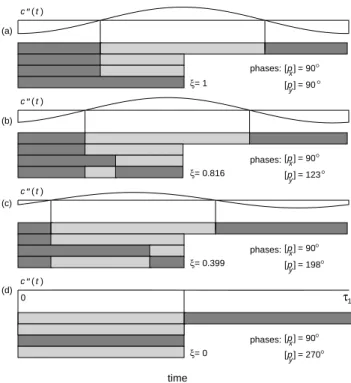
c " ( t )
ξ= 1
phases: [px] [p
y] = 90
= 90
° °
c " ( t )
ξ= 0.816
phases: [px] [p
y] = 90
= 123
° °
c " ( t )
ξ= 0.399
phases: [px] [p
y] = 90
= 198
° °
c " ( t )
ξ= 0
phases: [px] [p
y] = 90
= 270
° °
time 0
(a)
(b)
(c)
(d)
τ 1
Figure 10. Zero-crossing patterns defined in the second derivative
c′′(t)of a1: 1-complex having equal-amplitude components for different phase relationships. (a) The full symmetry(ξ= 1)gives the greatest resulting amplitude. This occurs when the phases are such that
[px] = [py] = 90◦. (b) With phases[px] = 90◦,[py] = 123◦, the
resulting amplitude is smaller as a consequence of a smaller symmetry
(ξ= 0.816). (c) With phases[px] = 90◦,[py] = 198◦, the resulting
amplitude is still smaller, due to a still smaller symmetry(ξ= 0.399). (d) A null symmetry(ξ= 0)gives a null resulting amplitude.
2.3.2. The symmetry in the1: 1-complex : The zero-valued symmetry only occurs in the 1: 1-complex. Al-though in perceptual terms a1: 1-complex is considered more as a single tone than as a complex, it plays a basic role in theoretical terms, not only for revealing how the symmetry of the zero-crossing pattern ofc′′
(t)affects the resulting loudness, but also for being a kind of unity ele-ment of the class ofm:n-complexes. Figure 10 shows the relationship between the pattern symmetry and the ampli-tude of the resultant sinusoid in a1: 1-complex.
3. V
ECTORR
EPRESENTATION OFT
ONESThe addition of two pure tones according to Equa-tion (3) results in a different entity because a complex has properties not present in pure tones. However, as men-tioned in Section 1, it is hypothesized that a computable pure tone exists whose frequency corresponds to the pitch of the complex. This hypothesis leads to the consideration of a mathematical model whose addition operation when applied to a pair of sinusoidal tones just yields a single
sinusoidal tone, instead of a superposition of sinusoidal functions, so that the pitch problem can be formalized in this way. For this purpose, it is first necessary to arrange the tones in a three-dimensional mathematical space.
3.1. THEQOLSPACE
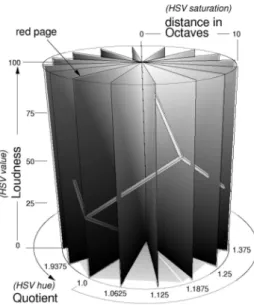
One way of organizing spatially the tones is through the rectangular QOL space shown in Figure 11 where tones are arranged inpages. More specifically, QOL is a space of tones having three dimensions, namely quotient, distance in octaves, and loudness, where all the tones be-longing to a same page have the same quotient.
Figure 11. Rectangular QOL organization of tones into pages, each of them corresponding to a different quotient in the range1≤q <2.
Each page is a Cartesian coordinate system of distance in octaves versus loudness, that is, a rectangle where all tones having the same
quotient are located. (Color online at http://www.cic.unb.br/docentes/arcela/cpv/f11.eps )
3.1.1. Building QOL from AFP: In order to set proper limits to the quantities involved in the AFP rep-resentation of Equations (1) and (2), it is assumed a lin-ear working of the auditory system, where the frequencies can have any value in the range ofN octaves, i.e., from
fmin to2Nfmin(for theoretical purposes,N is assumed
to be ten); the amplitudes can assume any value between zero and the limit given by Equation (35); and the phases, any value in the range from 0 to360◦
. For eachha, f, pi
triple, that is, for each tone with amplitudea, frequency
f, and phasep, there is a correspondinghq, o, litriple in QOL, and vice versa, so that there is a bijective transfor-mation between AFP and QOL spaces.
octavesνexisting betweenfminandf, i.e.,
q= f
2νfmin, (30)
whereνis given by
ν = int ·
log2
µ f
fmin ¶¸
. (31)
The term “quotient” as employed here has a meaning sim-ilar to that of “tone chroma” [4] in that both refer to the tone position within an octave. For example, notes hav-ing the same name also have the same chroma as well as the same quotient, regardless of the octave in which they are located. In color theory, however, the term “chroma”, which was introduced by Munsell [14], has a meaning that could result in a conflicting terminology if both tone and color spaces are used together, as occurs in the present study. In view of this, the term “chroma” is avoided.
The distance in octaves (o) of a tone is a quantity given by the number of octaves separatingf fromfmin
plus a fractional part due to the phasep. Therefore, it lies in the range0 ≤ o < 10. This definition of distance in octaves may be illustrated by means of the helix of pitch [23] shown in Figure 12, where the integer part is given by the number of turns fromfmintof, since each turn of the helix counts as one octave. In Figure 12(a), the helix is at the normal angular position, that is, its lower end is at zero radian. A tone in the normal helix is assumed to have a null phase. Starting atfminand going up to the higher frequencies, the helix intersects a certain horizontal cir-cle (a cross section of the helix’s circumscribed cylinder) defining the position of frequencyf at a pointp0. If the tone has a non-null phasep, as indicated in the same hori-zontal circle, the whole helix must be rotated bypradians so as to reach that circle exactly at pointp, as shown in Figure 12(b). In summary, the number of octavesνgives the integer part of the distance in octaves, while the dec-imal part is given by the quotient between the phase and the maximum possible rotation in the helix, i.e.,
o=ν+ p
2π . (32)
The concept of distance in octaves is thus like that of “tone height” found in [4]. However, since the phase is included, the distance in octaves is based on a continuous scale, instead of a discrete one.
Finally, theloudness dimension(l)is built in accor-dance with the definition presented in Section 2.2.1. In order to be included as one of the dimensions of the QOL tone space, the loudness must be rescaled to the range 0-100 loudness units. Therefore, it follows from Equa-tion (20) that
l= 100
µaf2
imax 
, (33)
whereimaxis the upper limit of the loudness scale, that is, a value above which the auditory system loses linearity. It is given by
imax=amaxfmin2 , (34)
wherefmin is the frequency corresponding to the lower limit of pitch discrimination, andamaxis the largest am-plitude which is supported by the auditory system under linearity conditions atfmin. If the equilibrium theorem is taken along the whole audible frequency range rela-tively to Equation (34), the corresponding amplitude (a) at a given frequency (f) is such that
a≤imax
f2 . (35)
The loudness unit—orlut for short—for the scalel de-fined in Equation (33) is derived from the assumption that a tone with frequency fmin and amplitude amax has a loudness of 100 luts. That is to say, at five octaves above
fmin, for example, a tone with 100 luts of loudness has an amplitude equals to(1/1024)amax.
frequency
octave count
p0
p0
0 1 2 3
0
f min 2f min
f 4f min 8f min
(a) normal position (b) rotated helix
phase amount
∆p p p
Figure 12. A geometric interpretation of distance in octaves by means of the helix of pitch. (a) The whole number of turns separating the lower limit of pitchfminfrom the frequencyfof the tone. (b) The
inclusion of phase in the helix of pitch is such that its effect is to rotate the whole helix by an angle corresponding to its magnitude.
3.2. THEQOLTORGBTRANSFORMATION
cannot be mathematically combined from a coordinate-by-coordinate addition, for example. However, the QOL space can be mapped onto the RGB color space—where the addition operation can be carried out—if, as a first step, its rectangular organization is converted to a cylin-drical one. That is, by transforming the quotientq, which lies in the range1 ≤ q < 2, into an angle lying in the range0−360◦
, a cylinder of pages is defined according to Figure 13 as having the same organization as that of the HSV color space. More specifically, by conveniently po-sitioning, scaling, and orienting the RGB cube relatively to the QOL cylinder, a correspondence is established be-tween quotient and hue, distance in octaves and satura-tion, and loudness and value. Here the cylinder’s axis coincides with the achromatic diagonal KW of the cube, which is aligned with the vertical direction; the radius of the cylinder’s base is equal to the projection of the vector
Y =R+Gon the horizontal plane; and thered page(the QOL page defined byq = 1) contains the edge KR of
the cube. Although the angular spacing of QOL pages is continuous, only a discrete set of pages is shown in order to render the inner side of the volume visible.
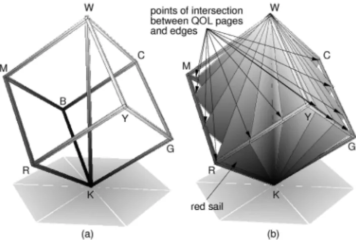
The QOL to RGB transformation requires a mapping of every page of the cylinder into a corresponding verti-cal triangle enclosed in the RGB cube, referred to here as sail, which is defined by the pointsK,W, and the inter-section point of the corresponding QOL page and one of the edgesRY,YG,GC,CB,BM, orMR, of the cube, as shown in Figure 14. That is, each tone of a given QOL page is mapped into a vector of the corresponding RGB sail. This can be done by taking advantage of the analogy between QOL and HSV, so that a QOL to HSV transfor-mation must be carried out first.
3.2.1. The QOL to HSV transformation: As the ge-ometries of QOL and HSV spaces are coincident, the con-version of ahq, o, litone to ahh, s, vicolor is according to
h= 360 (q−1), (36)
s= o
10, (37)
and
v= l
100. (38)
Therefore, the ranges are0≤h <360◦
,0≤s≤1, and
0≤v≤1.
3.2.2. The HSV to RGB transformation: A pair of algorithms allowing forward and inverse transformations between HSV and RGB color spaces was introduced by Smith [24]. Such algorithms are based on the “hexcone” representation of the HSV space which is equivalent to the cylindrical one. In this way, letΓ(hh, s, vi, k)be the
Figure 13. RGB-cube positioning, scaling, and orienting inside the QOL cylinder in a way that its achromatic diagonal coincides with the vertical axis of the cylinder. The vertexRof the cube is positioned on the surface of the cylinder in the same plane as the cylinder[0◦]-page (the red-page, i.e., whereq= 1). In this way, the vertexGis positioned
on the[120◦]-page, whereq= 4/3; and the vertexBis positioned on the[240◦]-page, whereq= 5/3. Although the cylinder is shown with a finite number of pages, the angular spacing is continuous, so that to
any quotient between 1 and 2 there is a corresponding page. (Color online at http://www.cic.unb.br/docentes/arcela/cpv/f13.eps)
Smith’s HSV to RGB algorithm, where each one of the coordinatesr,g, andbis indexed byk. That is,
r= Γ(hh, s, vi,0), (39)
g= Γ(hh, s, vi,1), (40)
and
b= Γ(hh, s, vi,2). (41)
The convention adopted here in relation to these algo-rithms is that found in [30] where the hue is taken in de-grees, that is, from0to360◦
, instead of0to1.
Figure 14. (a) RGB cube with its achromatic diagonal (defined by the verticesKandW, which correspond respectively to the colors black and white) aligned with the vertical direction. Indication of the vertices
R,G,B,C,M, andYwhich correspond respectively to the colors red, green, blue, cyan, magenta, and yellow. (b) Illustration of some sails as the result of the transformation of some QOL pages into RGB. The red
sail contains the vertexR. (Color online at http://www.cic.unb.br/docentes/arcela/cpv/f14.eps)
4. T
HEV
ECTORA
DDITIONT
ONE The purpose of applying the mathematical equiva-lence between a tone space and a color space in the com-putation of the pitch of a given complex is that it becomes possible to find a single tone as the final result of adding vectorially the respective component tones. Naturally, this is done in analogy with the addition—or mixing— of colors in the RGB cube, which is an operation that necessarilly results in a single vector, since regardless of the number of colors being mixed together, a single color must be produced at the end of the mixing procedure. In other words, the approach to compute pitch which is pre-sented here could not be proposed if the addition of tones were done by means of common algebraic addition of sine functions.Therefore, the methods introduced in Section 3 for representing tones as vectors are now combined so as to compute pure tones having supposedly pitch equivalence with harmonic complexes. The basic operation is the vec-tor addition of a pair of tones, which is carried out by Al-gorithmAas described below. For complexes with more than two components, the computation is carried out by AlgorithmM, which is described in Section 4.2. Multi-tone complexes are broken into several temporarym:n -complexes, so as to be resolved by successive applications of AlgorithmA, each of them producing a vector addition tone referred to as a temporary component.
4.1. THE VECTOR ADDITION OF TWO TONES
The computation of the vector addition tone for a
m:n-complex requires a sequence of three basic
oper-ations, namely down-transposition, vector composition, andup-transposition which are respectively carried out by the algorithmsD,C, andU described below.
4.1.1. Down transposition: The need for this oper-ation is due to the nature of the angular representoper-ation of tones in the QOL space, for the transformation given by Equation (36) which maps quotients into hues is not linear. For instance, if the lower component of a 2: 3 -complex is such thatfx/fmin is a power of two, so that the lower and upper quotients are respectively qx = 1
andqy = 1.5, the QOL page offxis the same as that of
fmin. Hence, according to Equation (36), the angular dif-ference between the HSV page of the upper component
y(t) and that of the lower componentx(t)is 180◦ , for
hy = 360(1.5−1) = 180◦
andhx= 360(1−1) = 0◦ , so that∆h = 180◦
. This means that the resulting vec-tor will be found on one of the two pages since they are in the same plane (Section 5.2). Now, whenfx/fminis not a power of two, the angular difference is not180◦
, as can be seen with a 2: 3-complex having qx = 1.25. In this case, the quotient of the upper component isqy = 1.25(3/2) = 1.875, so thathy = 360(1.875−1) = 315◦
, andhx= 360(1.25−1) = 90◦
, i.e.,∆h= 225◦
, and not
180◦
as in the first case. Therefore, in order to have a vec-tor composition as a homogeneous operation with respect to the frequency ratiom:n, and whose result does not de-pend on the value set tofmin, the down transposition is a required operation.
After the down-transposition operation, both lower and upper components will have their parameters changed in a particular way. More specifically,x(t)becomesx¯(t)
by first dividing its frequencyfxby its quotientqx, so that
¯
x(t)will be a component having a unitary quotient, that is,q¯x= 1, whiley(t)becomesy¯(t), a component which
is lowered by the same factor qx, so that the frequency ratiom:nis held. Next, the amplitudes are increased in the proportion given by the equilibrium theorem so as to preserve the loudness of both components. Finally, the phases are transformed in such a way that the transposed lower componentx¯(t)has its phase set toπ/2rd, while the phase of the transposed upper componenty¯(t)is set to a value at which the waveform of¯x(t) + ¯y(t)assumes— in a different time scale—the same shape as that of the waveform ofx(t) +y(t), as shown in Figure 15. The pur-pose of this phase transformation is to have a reference for measuring the waveform’s symmetry with Algorithm
S (Section 2.3.1), since a m:n-complex whose compo-nents are both in cosine phase is symmetrical.
Algorithm D(Down transposition algorithm). Given a
m:n-complex whose lower and upper components are, respectively, [x]AF P = hax, fx, pxi and [y]AF P = hay, fy, pyi, find the transposed components[¯x]AF P = ha¯x, fx, p¯ x¯iand[¯y]AF P =hay, f¯ y¯, py¯i.
step D1.[Find the quotient of the lower component.] Use Equations (30) and (31) to findqx.
step D2.[Down-transpose the lower component.] Find the frequency fx¯ of the down-transposed lower compo-nentx¯(t)by dividingfxby the quotientqx, that is,
fx¯= fx
qx. (42)
Then, find the amplitudeax¯by considering that the trans-posed component ¯x(t) must have the same loudness as
¯
x(t). That is, by applying Theorem 1,
a¯x=ax µfx
fx¯
¶2
. (43)
Now set the phasepx¯toπ/2. That is,
px¯= π
2. (44)
step D3.[Down-transpose the upper component.] Find the down-transposed upper componenty¯(t)according to
fy¯= fy
qx, (45)
ay¯= ly f2
¯ y
, (46)
and
py¯=py−
³n
m ´
px,¯ (47)
where the relationship betweenpx¯andpy¯is the same as that ofpxandpy.
4.1.2. Vector composition: This operation is applied to the transposed componentsx¯(t)and y¯(t). After ob-taining the symmetry ξ of the zero-crossing pattern of the second derivative of the transposed complexc¯(t) = ¯
x(t) + ¯y(t), which is the same as that of the untransposed complexc(t), it finds the vector composition of the two transposed tones as a vector addition under a magnitude coefficientξas described below.
AlgorithmC(Vector composition algorithm). Given the transposed tonesx¯(t)andy¯(t), find their vector composi-tion[¯u]RGB.
step C1.[Convert to QOL.] Convert the transposed components [¯x]AF P = ha¯x, fx, p¯ x¯i and [¯y]AF P = hay, f¯ y, p¯ y¯iinto QOL by using Equations (30)–(33). step C2.[Convert to HSV.] Convert the transposed com-ponents[¯x]QOL =hqx, o¯ x, l¯ x¯iand[¯y]QOL =hqy, o¯ y, l¯ y¯i into HSV by using Equations (36)–(38).
step C3.[Convert to RGB.] Convert the transposed components [¯x]HSV = hhx, s¯ x, v¯ x¯i and [¯y]HSV = hhy¯, sy, v¯ y¯iinto RGB by using Equations (39)–(41). step C4.[Find the symmetry.] Apply AlgorithmS (sym-metry algorithm; Section 2.3.1) to the transposed tones
¯
x(t)andy¯(t)in order to find the symmetryξof the zero-crossing pattern of¯c′′(t) = ¯x′′(t) + ¯y′′(t)
, i.e.,
ξ=S(¯x, y¯). (48)
step C5.[Add the vectors.] Find the transposed vector composition[¯u]RGB by using the symmetryξas a scalar
multiplier to the vector addition[¯u∗]
RGB = [¯x]RGB + [¯y]RGB. That is,[¯u]RGB=ξ[¯u∗]RGB, or
ru¯=ξ(rx¯+ry¯), (49)
gu¯=ξ(g¯x+g¯y), (50)
and
bu¯=ξ(bx¯+b¯y). (51)
4.1.3. Up transposition: The up transposition, which is the inverse operation of the down transposition, is ap-plied to the down transposed vector[¯u]RGB in order to
find and place the resulting tone u(t)in respect to the original untransposed tones x(t) andy(t), as shown in Figure 17. Before the up transposition is effectively ap-plied, the vector[¯u]RGB is first converted from RGB to
HSV, then to QOL, and finally to AFP.
AlgorithmU(Up transposition algorithm). Let Γ−1(hr
¯
u, gu, b¯ u¯i, k) represent the k-th component (0≤k≤2) of the RGB to HSV transformation.
step U1.[Go back to HSV.] Find the componentshu¯,su¯. andv¯u, by using
hu¯= Γ−1(hru, g¯ u, b¯ ¯ui,0), (52)
su¯= Γ−1(hru, g¯ u, b¯ u¯i,1), (53)
and
vu¯= Γ−1(hru, g¯ u, b¯ u¯i,2). (54)
step U2.[Go back to QOL.] Use Equations (55)–(57), which are derived from Equations (36)–(38), to convert the above computed HSV values back to QOL:
qu¯= 1 + h¯u
360, (55)
ou¯= 10su,¯ (56)
and
lu¯= 100vu.¯ (57)
vector addition toneu¯(t) =au¯sin(2πfut¯ +pu¯)by calcu-lating first the frequencyf¯u, then the amplitudeau¯, and finally the phasepu¯, that is,
fu¯=qu¯2int(ou¯)fmin, (58)
whereint(ou¯)is the integer part ofou¯. The amplitudeau¯ is then given by
au¯= imaxlu¯
100f2 ¯ u
, (59)
and the phasep¯ucomes from
p¯u= 2π[ou¯−int(ou¯)]. (60)
step U4.[Transpose the tone up.] Find the vector addition tone [u]AF P = hau, fu, pui by up transposing [¯u]AF P
under the factor1/qx. From Equations (45)–(47) used to down transpose the toney(t), the equations for the up transposition of toneu(t)can be deduced. They are
fu=qxfu,¯ (61)
au=au¯
µ fu¯ fu
¶2
, (62)
and
pu=p¯u+ (px−px¯)
µfu
fx 
, (63)
wherefuis the computed pitch.
4.1.4. Grouping the algorithms: At this point, the above described algorithms D, C, and U are combined together so as to define the algorithmAfor computing the vector addition of two tones, as illustrated in Figure 18.
AlgorithmA(Vector addition tone algorithm) Given the components x(t) andy(t) of a m:n-complex, find the vector addition toneu(t).
The componentsx(t)andy(t)are expressed in AFP quantities, that is,[x]AF P =hax, fx, pxiand[y]AF P = hay, fy, pyi, where the phases are in degrees.
step A1.[Do the down transposition.] Apply Algorithm
D to the components x(t) and y(t) so as to find the transposed tones[¯x]AF P = ha¯x, fx, p¯ ¯xiand[¯y]AF P = hay, f¯ y, p¯ y¯i.
step A2.[Do the vector composition.] Apply Algorithm
C to[¯x]AF P and[¯y]AF P so as to obtain the transposed
vector composition[¯u]RGB =hru, g¯ u, b¯ u¯i.
step A3.[Do the up transposition.] Apply AlgorithmU
to[¯u]RGBso as to find the vector addition tone[u]AF P = hau, fu, pui.
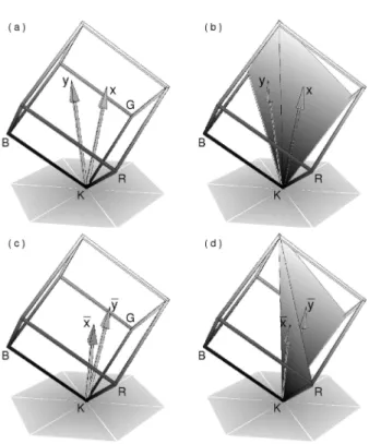
Figure 15. The down transposition of am:n-complex. (a) Waveforms of the spectral componentsx(t) = 2 sin[2π(468)t]and
y(t) = 1.3 sin[2π(585)t+ 216(π/180)]. (b) The corresponding 4:5-complex, that is,c(t) =x(t) +y(t). (c) The transposed componentsx¯(t)andy¯(t). (d) The transposed complex has a period
1.22(the approximate value ofqx) times greater than that of the
untransposed complex and, while it is phase shifted, its waveform has the same shape as the untransposed complex. (Color online at
http://www.cic.unb.br/docentes/arcela/cpv/f15.eps)
4.2. COMPLEXES HAVING MORE THAN TWO TONES
For complexes having more than two components, the vector addition tone is found by extending the application of Algorithm A to all the components of the complex. More specifically, the first two vector tones are added to-gether, the sum of which is added to the third component vector, and so on.
Algorithm M (Vector addition tone algorithm for har-monic complexes having more than two tones). Let
C(t) = {z0, z1, . . . , zk−1} be a complex having k har-monic components. Find the vector addition tone u(t)
by sequentially applying AlgorithmAto pairs of tones as follows:
step M1.[Add up the first two spectral components.] Find the first temporary componentu1(t)for the vector addi-tion tone by applying AlgorithmAto the first two spectral components, that is,
u1(t) =A(z0, z1). (64)
step M2.[Add up the remainder components.] Compute each iteration of the following operation sequence
uj(t) =A(uj−1, zj) ; for 2≤j < k, (65)
Figure 16. A pair of tones inside the RGB cube. (a) The vector representation for the tonesx(t) = 2 sin[2π(468)t]and
y(t) = 1.3 sin[2π(585)t+ 216(π/180)]. (b) The sails forx(t)on the right and fory(t)on the left. (c) The vector representation for the transposed tonesx¯(t)andy¯(t). (d) The sails for¯x(t)and fory¯(t). (Color online at http://www.cic.unb.br/docentes/arcela/cpv/f16.eps)
gives the resulting vector addition tone of the complex
C(t), i.e.,
u(t) =uk−1(t). (66)
This ends the algorithmM.
5. G
EOMETRY OFC
OMPLEXESThere is a close relationship between the geometry of any vector composition and the corresponding reduced harmonic numbers m, nfrom which relevant properties related to the pitch of complexes can be derived. Some of these properties refer to the problem of the missing fun-damental. In this way, in order to address the conditions of equality between the computed pitch and the frequency of the fundamental, four basic frequency ratios are stud-ied here.
5.1. COMPONENTS AN OCTAVE APART
According to Equation (31), in a two-tone complex whose components are one octave apart, that is,m:n = 1: 2, the difference between the number of octaves of the transposed toney¯(t)relatively tofminand that ofx¯(t)is
νy¯−ν¯x= 1. (67)
Figure 17. Up transposition. (a) The transposed vector addition tone
¯
u(t)of componentsx(t) = 2 sin[2π(468)t]and
y(t) = 1.3 sin[2π(585)t+ 216(π/180)]. (b) The up transposition operation gives the final vector addition toneu(t), where the frequency
is multiplied by the quotientqxof the original lower tone so that the
resulting tone has a period in the same scale of time as that of the original complex. (Color online at
http://www.cic.unb.br/docentes/arcela/cpv/f17.eps)
As shown in Figure 19(a) for the respective vector com-position, since the RGB sails of both transposed tones are coincident, that is,
qx¯=qy¯= 1, (68)
the transposed addition tone will be located on this com-mon sail. That is to say, any quotient the lower tone
x(t)might have, which is always equal to that of y(t), the vector-addition toneu(t)will have the same quotient (Section 4.1.4, step A3), that is, qu = qx. However, mainly due to the phase relationship and secondarily due to the amplitude proportion, the resulting pitch can be ei-therfx orfy. For instance, when the1: 2-complex is in equilibrium, that is,
lx¯=ly,¯ (69)
the transposed vector addition toneu¯(t)has a distance in octavesou¯equal to the arithmetical mean of the distances in octavesox¯andoy¯of the transposed componentsx¯(t) andy¯(t). As a consequence, if the phasepxis set toπ/2
rd whilepy can assume any value between0 and2πrd, the pitch will correspond tofx when 0 ≤ py < 3π/2, and will correspond tofy when3π/2 ≤py <2πrd, as demonstrated below.
The HSV equivalents of Equations (68) and (69) are given respectively by Equations (36) and (38), that is,
Figure 18. Vector composition of tones. (a) The vector representations
[¯x]RGB,[¯y]RGB, and[¯u]RGBof the componentsx(t)andy(t)along
with and transposed vector addition toneu¯(t). (b) The sails of
[¯x]RGB,[¯u]RGB, and[¯y]RGB(the latter is not visible in the figure).
(c) The vector representation[¯u]RGBof the vector addition toneu(t)
of the componentsx(t) = 2 sin[2π(468)t]and
y(t) = 1.3 sin[2π(585)t+ 216(π/180)]. (d) The sails for[x]RGB,
[x]RGB, and for the addition vector[u]RGB. Here, a180◦rotation
has been applied to the cube so as to make all the three sails visible. (Color online at http://www.cic.unb.br/docentes/arcela/cpv/f18.eps)
and
vx¯=vy¯= lx¯
100. (71)
In terms of RGB coordinates, the necessary conditions for a vector to be located on the red sail are that (1) the coordinates g and b are equal, and (2) the coordi-nate r is the greatest among the three, that is, rx¯ = max(rx, g¯ ¯x, bx¯)and r¯y = max(ry, g¯ y, b¯ y¯). Therefore, according to the HSV to RGB transformation represented by Equations (39)–(41) and the conditions indicated by Equations (70) and (71), the transposed RGB vectors can be obtained. The vector [¯x]RGB is given by rx¯ = vx¯, gx¯=vx¯(1−sx¯), andbx¯=gx¯, that is,
r¯x= l¯x
100, (72)
gx¯= lx¯ 100
³
1−o10x¯´, (73)
and
bx¯=gx.¯ (74)
In the same way, the vector[¯y]RGBis given by
ry¯= lx¯
100, (75)
g¯y= lx¯ 100
³
1−o10y¯´, (76)
and
b¯y=gy.¯ (77)
From Equations (72)–(77), the coordinates of the trans-posed resulting vector[¯u]RGB =hrx¯+ry, g¯ x¯+gy, b¯ x¯+ by¯iare given by
ru¯= lx¯
50, (78)
gu¯= lx¯ 100
µ
2−ox¯10+oy¯ 
, (79)
and
bu¯=gu.¯ (80)
In order to find the distance in octavesou¯, first the satu-rationsu¯ must be obtained from the RGB to HSV trans-formation indicated by Equations (52)–(54), that is,su¯= [max(r¯u, gu, b¯ u¯)−min(ru, g¯ u, b¯ u¯)]/max(r¯u, gu, b¯ u¯). As the maximum isru¯and the minimum isgu¯, it follows that
su¯=
ru¯−g¯u ru¯
. (81)
Substitutingsu¯ =ou/¯ 10, as given by Equation (37), to-gether with Equations (78)–(79) into Equation (81) yields
ou¯=
ox¯+oy¯
2 , (82)
which, according to Equation (32), can be rewritten as
ou¯= 1 2
³ νx¯+
px¯
2π+νy¯+ py¯ 2π ´
. (83)
Now, taking into account Equation (67) yields
ou¯=νx¯+ 1 2+
px¯+py¯
4π . (84)
Therefore, if
1 2+
p¯x+py¯
4π ≥1, (85)
that is, ifpx¯+py¯≥2π, the number of octavesνu¯of the transposed vector addition tone will be 1 plus the number of octavesνx¯, so that the resulting pitch equalsfy. Oth-erwiseνu¯will be equal toν¯x, and so the pitch will befx.
For example, ifpxis set toπ/2which, according to Equa-tions (44) and (47), implies in a equality betweenpxand
p¯xas well as betweenpyandpy¯, then for0≤p¯x<3π/2,
Figure 19. Vector composition of transposed components of
m:n-complexes having simplem:nratio. (a) Vector addition of tones in octaves. (b) Vector addition of tones in fifths. Definition of the red-cyan rectangular section. (c) Vector addition in fourths. (d) Vector
addition in major thirds. (Color online at http://www.cic.unb.br/docentes/arcela/cpv/f19.eps)
5.2. COMPONENTS A FIFTH APART
For a complex whose components are a fifth apart, that is,m:n = 2: 3, the vector placement is that shown in Figure 19(b). In this case, the sails of the transposed tones are complementary, so that the association of them defines the red-cyan rectangular section of the RGB cube. Because of this singular alignment of sails, the transposed resulting vector[¯u]RGBwill be located exclusively either
on the sail of[¯x]RGBor on that of[¯y]RGB. As illustrated
in Figure 20 for the red-cyan rectangular section, if the angle ψbetween the transposed addition vector[¯u]RGB
and the diagonal KC (of the face KBCG) is greater than
δ= tan−1(√2/2)—the angle between the diagonal KW of the cube and the diagonal KC of the face—the result-ing vector will be on the red sail, so that its quotient will be the same as that of[¯x]RGB. Otherwise, it will be on
the cyan sail, and so its quotient will be equal to that of
[¯y]RGB.
Since the necessary condition for a RGB vector to be located on the red-cyan rectangular section is that its com-ponentsgandbhave the same value, it holds for the
vec-tor[¯x]RGB thatgx¯ = bx¯, while for the vectory¯it holds thatgy¯=by¯, so that the projection of the resulting vector [¯u∗]
RGBon the side KR is given by
ru¯∗ =rx¯+r¯y, (86)
while its projection on the diagonal KC is
cu¯∗ = (g¯x+g¯y)
√
2. (87)
Therefore, as
tanψ= r¯u∗ cu¯∗
, (88)
the resulting vector will be located on the red sail if
rx¯+ry¯ (g¯x+gy¯)
√ 2 >
√ 2
2 , (89)
that is,
rx¯+r¯y> gx¯+gy,¯ (90)
whereas it will be located on the cyan sail if
rx¯+r¯y< gx¯+gy.¯ (91)
5.2.1. Computed pitch under equilibrium: When the
2: 3-complex is in equilibrium, that is,l¯x=l¯y, it follows
from Equation (57) that
vx¯=vy¯, (92)
a condition whose RGB equivalent is found from the RGB to HSV transformation mentioned in Section 3.2.2 according to which vx¯ = max(rx, g¯ x, b¯ x¯), and vy¯ = max(ry¯, gy¯, b¯y). Therefore, since
max(r¯x, gx, b¯ ¯x) =r¯x (93)
and
max(ry, g¯ y, b¯ y¯) =gy¯, (94)
it holds that
r¯x=gy.¯ (95)
Substituting Equation (95) into Equation (90) gives the condition for the transposed resulting vector being located on the red sail, that is,
r¯y> gx.¯ (96)
Substituting Equation (95) into Equation (91) gives the condition for the transposed resulting vector being located on the cyan sail, that is,
r¯y< gx.¯ (97)
[max(r¯y, gy¯, by¯) − min(ry, g¯ y, b¯ y¯)]/max(ry¯, gy, b¯ ¯y).
Since min(rx, g¯ x, g¯ ¯x) = g¯x andmin(ry, g¯ y, g¯ y¯) = ry¯, and by using Equations (93)–(95), it follows that
s¯x=
rx¯−gx¯ rx¯
(98)
and
sy¯=
r¯x−ry¯ r¯x
. (99)
To find the condition for the transposed resulting vector being on the red sail under equilibrium, it is necessary to compare Equations (98) and (99) one to the other while taking into consideration Equation (96). In this way, it follows thatsx¯ > s¯y, or, according to Equation (56), the
respective distances in octaves are such that
o¯x> oy¯, (100)
which, from Equation (32), yields
νx¯+ px¯
2π > ν¯y+ py¯
2π. (101)
Sincef¯xis a power of two timesfmin, it follows from
Equations (30) and (31) thatf¯x andfy¯are in the same octave relatively tofmin. Therefore,
ν¯x=ν¯y. (102)
Then, substituting Equations (44) and (102) into Equa-tion (101), it follows that
py¯< π
2. (103)
That is, under equilibrium conditions of the2: 3-complex, the resulting transposed vector will be on the red sail if the phase of the transposed higher toney¯(t)is lesser thanπ/2
rd. Otherwise, that is, if
π
2 < py¯<2π, (104)
it will be on the cyan sail. Therefore, the pitch of a
2: 3-complex in equilibrium has a bipolar response to the phase relationship, since it can assume just one of two values, i.e., according to Equation (61), fminqx, when the transposed resulting vector is on the red sail, and
1.5fminqx, when it is on the cyan sail.
Finally, if both tones not only have the same loudness but also are in cosine phase, that is, the2: 3-complex is in entire equilibrium (Section 2.2), the resulting vector will be aligned with the achromatic diagonal KW, which is the border between the red and cyan sails. This means that in this very particular case, the resulting pitch is indefinite.
ψδ x
y u∗
u
K
C
R
W
s
s√2
g y√2
cu*
g x√2 r
x ru*
r y KR = side of the RGB cube = s
KC = diagonal of the face = s√2
KW = diagonal of the cube = s√3
KRW = red sail
KCW = cyan sail
ψ = resulting angle
δ = tan -1
(
√2 2)
≈ 35.26°Figure 20. A vector composition on the red-cyan rectangular section of the RGB cube where the resulting transposed vectoru¯is found on the
red sail. In this case, the vector addition tone will have the same quotient as that of¯x.
5.3. COMPONENTS A FOURTH APART
For a complex whose components are a fourth apart, that is,m:n= 3: 4, the placement of vectors is that shown in Figure 19(c). Now, as the sails of the transposed tones are angularly spaced apart by120◦
, the transposed result-ing vector[¯u]RGBcan be located on any sail defined
be-tween0and120◦
. Therefore, the quotient of the vector addition tone has a value between the component quo-tients.
When a 3: 4-complex is in entire equilibrium, the value of its computed pitch is an octave below the arith-metic mean of the component frequencies, that is,fu = (fx+fy)/4. (A proof of this statement is not given here). The effects of phase in this complex are described below in Section 5.5
5.4. COMPONENTS A MAJOR THIRD APART
For a complex whose components are a major third apart, that is, m:n = 4: 5, the placement of vectors is that shown in Figure 19(d). In this case, the sails of the transposed tones are angularly apart by 90◦
, so that the transposed resulting vectoru¯(t)can be located on any sail defined between0and90◦
. Therefore, the computed quo-tient is a value between the component quoquo-tients.
5.5. PHASE EFFECTS ON THE PITCH OF m:n -COMPLEXES
By keeping the phasepxat90◦
whilepyis allowed to vary from0to360◦
, it is possible in terms of phase sensi-tivity to classifym:n-complexes into four major groups according to the way the pitch changes in each of them.
the phase relationship, although the loudness of the vector addition tone is affected.
The second one is constituted of complexes having a bipolar effect, that is, those in which, for a certain phase subrange for py, the resulting pitch corresponds to one of the component frequencies, while for the complemen-tary subrange it corresponds to the other component fre-quency, as occurs with1: 2and2: 3complexes discussed above in Sections 5.1 and 5.2.
The third one comprises complexes whose pitch re-sponse has a discontinuity, that is, there are two comple-mentary phase subranges where pitch varies continuously, being these subranges about one octave apart one from the other. For example, the pitch of a4: 5-complex in equilib-rium increases continuously 44 cents relatively to a given frequency value as py goes from0to330◦
, while from
330to360◦
it increases continuously from1244to1247
cents relatively to the same reference value of the first subrange. Other examples include5: 6,22: 27, and 5: 8
complexes.
Finally, the fourth and last group comprises m:n -complexes in which the pitch varies continuously along the full phase range, in general for a small interval. For instance, the pitch of a 3: 4-complex in equilibrium in-creases continuously about 88 cents aspy goes from0to
360◦
, while a8: 9-complex in equilibrium increases about 20 cents. Other examples include25: 36,3: 5, and8: 15
complexes.
6. T
HEM
ISSINGF
UNDAMENTALThe application of Algorithm M to three examples selected from the literature is first considered. Subse-quently, the possibility for the pitch of a harmonic com-plex to be the same as the frequency of the fundamental is investigated by exploring the geometric properties of the vector pairs operated by AlgorithmA inside Algorithm
M. An audible demonstration of these complexes and their respective vector-addition tones is found in [3].
From this point on, the notation “Hk” for a spectral
component is used, which is intended to mean that the integerkis the harmonic number of the respective com-ponent, that is, fHk = kfH1, being Hk the same as
Hk(t) =aHksin(2πfHkt+pHk).
6.1. PITCH COMPUTATION FOR A COMPLEX WITH SUCCESSIVE HARMONICS
The complex C1 = {H3,H4,H5} to be considered in the first place has component frequencies according to 600, 800, and 1000 Hz, respectively, so that its miss-ing fundamental is at 200 Hz. A study of this com-plex was reported in [9] where the components H3, H4, and H5 have the same amplitude and are in
co-sine phase. Their values in AFP quantities are taken as
[H3]AF P = h0.9,600,90i, [H4]AF P = h0.9,800,90i,
and[H5]AF P =h0.9,1000,90i. In this way, their
loud-nesses are according tolH3 = 36,lH4 = 64, andlH5 =
100luts. The amplitudes are set to 0.9 units because this value is appropriate in relation to the upper limit ampli-tude of the highest componentH5, which is also the loud-est one. More precisely, for a lower limit pitchfmin set to 30 Hz [12] and an upper limit amplitude[amax]fmin
set to 1000 units, then according to Equation (34) the maximum loudness isimax= 900000. Therefore, it fol-lows from Equation (35) that the upper-limit amplitude forH3is[amax]fH3 = 900000/1000
2 = 0.9
units. As the amplitude values are relative to each other, overall gain adjustments are required for a suitable sound pres-sure level as, for example, a value around 65 dB SPL for
H5. The final vector addition tone is found by applying AlgorithmMto the set of the three components such that
u(t) = M(H3,H4,H5) = A[A(H3,H4),H5], that is, the Algorithm A is first applied to the components H3 andH4 thus yielding a temporary toneu1(t), then it is applied again, this time to the pair(u1,H5). In this way, the computed pitch for the complexC1is 229.145 Hz, that is, 236 cents above the 200-Hz fundamental. As for the loudnesslu, the computed toneu(t)has a loudness of 45 luts, therefore a value between the loudnesses ofH4and H5.
6.1.1. Phase sensitivity: Small changes in any of the phases of components H3, H4, and H5 produce small changes in the pitch of C1. There are, however, some phase relationships that produce significant changes in the pitch as, for example, when the phase ofH3is set to0◦ while those ofH4andH5 are held at90◦, the resulting tone is[u]AF P = h1.87,485.25,150i, that is, the
com-puted pitch is 1299 cents above that value found in the case where the components are all in cosine phase, with a loudness of 49 luts. If the phase ofH4 is set to180◦ while the phases ofH3andH5are held at90◦, the result-ing tone is[u]AF P =h0.65,983.88,199.17i, that is, the
pitch is 2523 cents above the first computed value, with a loudness of 70 luts.
6.2. ANOTHER COMPLEX WITH SUCCESSIVE HAR -MONICS
The complex C2 = {H9,H10,H11} to be consid-ered now was mentioned in [5]. It has component fquencies according to 1800, 2000, and 2200 Hz, re-spectively, so that its missing fundamental is at 200 Hz. In AFP quantities they are taken as [H9]AF P = h0.0675,1800,0i, [H10]AF P = h0.15,2000,0i, and [H11]AF P = h0.0675,2200,0iso that the
correspond-ing loudnesses arelH9 = 24,lH10 = 66, andlH11 = 36
[u]AF P = h0.21,2024.38,359.88i. Thus, the computed
pitch, that is, 2024.38 Hz, is 4007 cents above the fre-quency of the fundamental. The loudness is 97 luts.
6.3. A COMPLEX HAVING NONSUCCESSIVE HAR -MONICS
The complex C3 = {H46,H51,H56} to be consid-ered now was also mentioned in [5]. It has compo-nent frequencies according to 1840, 2040, and 2240 Hz, respectively, so that its missing fundamental is at 40 Hz. In AFP quantities they are taken as [H46]AF P = h0.0675,1840,0i, [H51]AF P = h0.15,2040,0i, and [H56]AF P = h0.0675,2240,0iso that the
correspond-ing loudnesses arelH46 = 25,lH51 = 69, andlH56 = 37
luts. After applying AlgorithmM toC3, it is found that [u]AF P = h0.11,2058.17,359.88i. Thus, the computed
pitch, that is, 2058.17 Hz, is 29 cents above the value found for the preceding complex. The loudness is 53 luts.
6.4. COMPUTED PITCH COMPARED TO THE FRE -QUENCY OF THE FUNDAMENTAL
The pitch computation for the complexes C1 andC2 above indicates that successive harmonics are not a nec-essary and sufficient condition to assure the equality be-tween pitch and the frequency of the fundamental. The same is true for nonsuccessive harmonics, as shown with complex C3. The equality between pitch and the fre-quency of the fundamental (whether present or missing) is discussed below through the pitch computation of some selected complexes, followed by the description of a well-defined class of harmonic numbers related to such equal-ity.
6.4.1. Complex having the first three harmon-ics. First case: the computed pitch is equal to the frequency of the fundamental: First, let C4 = {H1,H2,H3} be a complex having the first three har-monics. According to AlgorithmM, the vector addition tone of complexC4 can be found by two successive ap-plications of AlgorithmA, namelyu1(t) = A(H1,H2), andu2(t) =A(u1,H3). After generating the down trans-posed tonesH¯1andH¯2in the first step of AlgorithmD, since fH¯2 = 2fH¯1, it follows from Equation (30) that
qH¯1 = qH¯2 = 1. That is, the vectors [ ¯H1]RGB and
[ ¯H2]RGB are on the same RGB sail. Therefore, the
tem-porary componentu1(t)has the same quotient asH1, as discussed in Section 5.1 for a1: 2-complex. Now the sit-uation is like that described above in Section 5.2 for a
2: 3-complex. That is, if u1(t) when compared to H3 is such that Equation (89) holds, the resulting toneu2(t) will have the same quotient asu1(t), which is the same as that ofH1. Therefore, the computed pitch will be equal to the frequency of the fundamental. Otherwise, it will
have the same quotient asH3, for it will be on the page qu2 = qH3. In this case, the computed pitch will be the
same as a fifth above the frequency of the fundamental. For a direct numerical example, let the spectral components H1, H2, and H3 of C4 be [H1]AF P = h4,200,90i,[H2]AF P = h3,400,90i, and [H3]AF P = h0.34,600,90i. According to Equation (33), the cor-responding loudnesses are lH1 = 18, lH2 = 53, and
lH1 = 14 luts. After applying Algorithm M toC4, it
is found that [u]AF P = h16.89,200,55.39i. Thus, the
computed pitch—200 Hz—is the same as the frequency of the fundamental, the loudness being 75 luts.
6.4.2. Complex having the first three harmonics. Second case: the computed pitch is a fifth above the frequency of the fundamental: For a complexC5 hav-ing the same first three harmonicsH1, H2, and H3 as C4, but having another proportion of amplitudes, namely [H1]AF P = h3,200,90i, [H2]AF P = h1.05,400,90i,
and [H3]AF P = h2,600,90i—that is, the
correspond-ing loudnesses arelH1 = 13,lH2 = 17, andlH3 = 80
luts—after applying AlgorithmM toC5, it is found that [u]AF P =h7.25,150,152i. Thus, the computed pitch—
150 Hz—is a fourth below the frequency of the funda-mental, with a loudness of 18 luts.
6.4.3. Complex having the first four harmon-ics. First case: the computed pitch is equal to the frequency of the fundamental: Let C6 = {H1,H2,H3,H4} be a complex having the first fourth harmonics. According to Algorithm M, the vector addition tone of complex C6 can be carried out by three successive applications of Algorithm A, that is,
u1(t) = A(H1,H2), u2(t) = A(u1,H3), andu3(t) = A(u2,H4). If the components are such that[H1]AF P = h4,200,90i, [H2]AF P = h3,400,90i, [H3]AF P = h0.75,600,90i, and[H4]AF P = h0.5,800,90i—that is,
the corresponding loudnesses arelH1 = 18,lH2 = 53,
lH3 = 30, andlH4 = 36luts—after applying Algorithm
M toC6, it is found that[u]AF P = h22.35,200,167i.
Thus, the computed pitch—200 Hz—is the same as the frequency of the fundamental with a loudness of 99 luts.
6.4.4. Complex having the first four harmonics. Second case: the first three components have the same loudness; the computed pitch is one octave below the frequency of the fundamental: Let C7 = {H1,H2,H3,H4} be a complex having the first fourth harmonics. If the components are such that[H1]AF P = h6,200,90i, [H2]AF P = h1.5,400,90i, [H3]AF P = h0.65,600,90i, and[H4]AF P =h0.23,800,90i—that is,
the first three have the same loudnesslH1=lH2=lH3 =


![Figure 15. The down transposition of a m:n-complex. (a) Waveforms of the spectral components x(t) = 2 sin[2π(468)t] and y(t) = 1.3 sin[2π(585)t + 216(π/180)]](https://thumb-eu.123doks.com/thumbv2/123dok_br/18976836.455599/12.892.443.798.175.517/figure-transposition-complex-waveforms-spectral-components-sin-sin.webp)