Abstract---For improved estimation of oxygen tension in retinal blood vessels, regularization of least squares estimation method was proposed earlier and it was shown to be very effective. Optimum points of the regularized least squares (RLS) cost function were found using iterative methods and closed form solutions for the estimation, and bias and variance of the estimators were not provided. In this study, we derive the closed form solution for the RLS estimation and using the closed form solution we derive bias and variance of the RLS estimator. With the help of the bias and variance, statistical performance analyses of the RLS estimator are realized without the need of the Monte Carlo simulations and effective examinations of the regularization parameters on the performance become available. Therefore, preferable ranges for the parameters that can be adjusted during the acquisition and estimation can be found easily to have enhanced estimates.
Index Terms---performance analysis, bias and variance, regularized estimation, retinal oxygenation.
I. INTRODUCTION
Accurate estimation of oxygen tension (pO2) in retinal vessels is of primary importance since abnormality of oxygenation in retinal tissue, in many cases, gives important clues regarding devastating common eye diseases such as diabetic retinopathy, glaucoma, and age related macular degeneration [1]-[2]. Oxygen tension of retinal vessels can be estimated using phosphorescence lifetime imaging model (PLIM) [3]-[4] whose mathematical model was developed by Lakowicz et al. [5] for fluorescence lifetime imaging model (FLIM). In [3]-[4], the least squares (LS) estimation method was used to obtain estimate of oxygen tension in retinal vessels using PLIM. While the LS estimation method is efficient in the computation sense, it produces high variance, and artificial peaks in the estimates, and therefore gives values outside of the physiological range. In order to overcome these shortcomings, regularization of the LS estimation methodwas proposed by Yildirim et. al. [6].
Regularization has been extensively used in several problems such as image processing [7-9], biomedical imaging [10-13], and astronomical imaging [14] and its success in many problems was the main motivation of Yildirim et al. [6] to develop a RLS estimation method in the estimation of oxygen tension in retinal vessels
G. Gunay is with the Department of Electrical and Electronics Engineering, Bozok University, 66900, Yozgat, TR. (E-mail: ggunay@ itu.edu.tr).
I. Yildirim is with the Department of Electrical and Electronics Engineering, Istanbul Technical University, 34469, Maslak, Istanbul, TR. Yildirim is also with Master of Engineering Department, University of Illinois, Chicago, 60607, IL, USA. (E-mail: iyildirim@ itu.edu.tr, [email protected])
In their study, after considering the physiology of retinal tissue in which oxygen tension of a retinal vessel does not vary rapidly in a small neighborhood [15], they assumed that mean value of a pixel value in an oxygen tension map of retinal blood vessel can be formulated as equal to weighted mean of oxygen tension values of its neighboring pixels. It was shown that their RLS method is much better than the LS estimation approach in many senses such as robustness to noise, having much less variance, obtaining smoother pO2 maps and therefore generating pO2 values
which are in the physiologically expected range. However, in their study, iterative procedures such as steepest descent algorithm were used to find minimum of the RLS cost function and a closed form solution was not provided. Bias and variance of the estimator were also estimated using some Monte-Carlo simulations.
In this study, we derive bias and variance of the RLS estimator after obtaining closed form solution of RLS estimation method proposed in [6]. With the help of the bias and variance of the RLS estimator, we examined and showed the effects of the regularization parameters, window size and weighting coefficients of neighboring pixels, which are used in formation of regularization term in the model, and phosphorescence observation number on the statistical performance of the estimator. Considering the outcomes of the analyses, we give the preferable ranges for the parameters that can be controlled to generate the pO2 maps.
II. DERIVATION OF THE CLOSED FORM SOLUTION FOR THE RLS ESTIMATION
Phosphorescence intensity observation images are represented in a vector form by reordering the matrix elements column wise. For the ith pixel, the RLS cost function can be given as follows:
, (1)
where , and stand for noise corrupted observation vector, regularization coefficient and the system matrix (see Appendix A). Additionally, the parameter to be estimated and its mean are as follows:
and
, : , : , : , (2) where , and are vectorized parameter values and K
is weighted mean averaging matrix defining interrelations between pixels’ , and parameters (see Appendix B). Since the regularization term in (1) involves all
Statistical Performance Analysis of the RLS
Estimator for Retinal Oxygen Tension Estimation
pixels’ , and parameters, there is no pixel-wise solution and the problem must be handled for all pixels. Therefore, the global RLS cost function is defined as:
∑ , (3) where M is number of pixels in the oxygen tension map.
Let ∈ , ‖ ‖ is called as Frobenius norm in space and
‖ ‖
∑ ∑ , (4)
where tr() denotes trace of inner matrix. The operation is called as Frobenius inner product [17].
Following that, the global cost function using Frobenius inner product can be given as follows:
‖ ‖ ‖ ‖ , (5) where A is the system matrix, is the regularization
coefficient and:
… … …
… …
… … … , … …
⋮ … ⋮ … ⋮ … … ⋮ … ⋮ … ⋮
… …
, (6)
where and S are respectively pth phosphorescence intensity observation for ith pixel and number of observation per pixel.
Considering the definition of the X, equations (2) and (5)
can be rewritten as follows:
, : , (7)
‖ ‖ ‖ ‖ . (8) For the PLIM parameters, the regularization term in the cost function (8) can be fragmented as follows:
‖ ‖
‖ ‖ ‖ ‖ ‖ ‖ (9) The data fidelity term in equation (8) can be rewritten as:
‖ – ‖
(10)
Since is as follows:
/
/ , (11)
where S is number of observation per pixel, becomes:
. (12)
Additionally, from the definition of the Frobenius inner product, can be rewritten as follows:
: , : , : , . (13)
Considering the equations above, the global cost function can be given as:
: ,
: , + : ,
‖ ‖ ‖ ‖ ‖ ‖ . (14)
Finally, after taking gradient of the cost function with respect to parameter and equalizing the gradients to zero, we get the RLS estimate of the parameters.
: ,
. (15)
Further, assuming that / , we can rewrite equation (15) as follows:
: , .
Finally, we get as:
: , . (16) Since the same procedure is followed, we use the results of the parameter for the parameter .
Considering the definition of and its pseudo-inverse, it is explicit that : , and : , are the LS estimates of the and parameters, respectively. Therefore, we can rewrite the RLS estimates of parameter as follows:
, (17)
To abbreviate the notation, we define a new matrix L as:
, (18)
where, Istands for the identity matrix.
Using the matrix L, the RLS estimates of the parameter
and can be rewritten in a simpler form as:
, (19)
. (20)
A. Bias for the LS and RLS Estimators
We modeled our observation corrupted by the additive zero mean i.i.d. Gaussian noise, therefore the expectation of the LS estimation becomes equal to:
. (21)
Following this fact and using (19), we can define the bias vector of the RLS estimator as:
(22) In order to facilitate visualization of the bias in graphs, we define a normalized scalar bias as follows:
B. Variance for the LS and RLS Estimators
Oxygen tension depends on ratio of the model parameters
b1 and a1 [6]. However, variance of this ratio cannot be found since ratio of two Gaussian distribution does not have a defined variance value [16]. In this regard, we only consider variance of a1 which is equal to variance of b1. We define the LS estimate of parameter vector as:
: , , (24)
where i denotes pixel number under consideration. Covariance matrix of the observation vector is equal to the covariance matrix of the noise.
: , ⋮ ⋮ …⋱ ⋮
… (25)
: , (26)
Since Var : , ,
/ /
/
. (27)
Considering parameters of i-th pixel, as can be seen from
Var x , cross-covariances of a , a and b are equal to zero and their auto-covariances are /S , σ /S and σ /S, respectively. Since there is no relationship between pixels in the LS estimation, auto-covariance matrix of a can be given as:
/ . (28)
Turning our attention to the RLS estimation, as shown above, a is equal to L a . Using this, we can write variance of a as:
/ (29)
IV. RESULTS
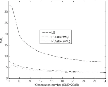
Fig.1. shows the simulated data and its estimates in the presence of noise with 20 dB SNR and a beta value of 10 using the (2) LS and (3) RLS methods, respectively. This simulated data is used to compare MAE performances of the LS and RLS estimators given in Fig. 3.
Fig.2. gives variance and normalized bias of the LS estimator and of the RLS estimator for different regularization window sizes and parameters. As the beta increases, variance of the RLS estimate decreases as expected. Variance of the LS estimate is 0.2 times the noise variance whereas for a beta value of 6 variance of the RLS estimator gets lower than 0.025 times the noise variance for 3x3 and gets lower than 0.012 times the noise variance for 5x5 window sizes. Increasing values of the regularization coefficient leads to increase in bias of the RLS estimation method as expected whereas helps to obtain lower variance values of the estimates. There exists a bias-variance tradeoff. Therefore, the beta cannot be selected arbitrarily large.
Between two different window sizes, we see that there is a slight superiority of 5x5 window size over 3x3 window size in the variance performance of the RLS estimation method.
However, in the bias sense, 3x3 performs considerably better than 5x5 window size. Therefore, in the sense of bias-variance performance of the RLS estimation method, 3x3 window size is more preferable than 5x5 window size.
Additionally, as can be seen from Figure 2 that for the beta values greater than 5, bias performance of the RLS estimation method decreases rapidly whereas there is a relatively slow improvement in the variance performance. In this regard, the beta values greater than 5 may not be recommended.
The phosphorescence intensity observation number which is an experimental set up parameter plays a key role in the performance of the estimators. As the observation number increases, performances of the both LS and RLS estimators increase in both MAE and variance of the estimate senses as shown in Figures 3 and 4. However, the experimental cost increases with the increasing number of the observation number.
Therefore, it cannot be chosen arbitrarily large. Since the change in the performance of the RLS estimation method gets less noticeable after the observation number 10, observation number may be selected around 10 depending on the experimental cost.
We also examined performance of the proposed method for different values of weighting coefficients in the regularization window that controls values of the matrix . In Figure 5, (1) and (2) denote the RLS estimates for two different 3x3 regularization windows’ l, p and q coefficients by considering the geometric distance and choosing regardless of the distance in the window as follows:
l p √ , (2) l p q ,
where l, p and q are the coefficient of the self, adjacent and cross-adjacent pixels, respectively. We see that considering variance performances of the RLS estimation method for two different regularization window weighting coefficients, there is a negligible difference. On the other hand, for increased beta, bias performance of the RLS estimation using the second type of window decreases faster than the one using the first type of window. Therefore, the first type of window becomes more preferable when compared with the second type of window as expected.
V. CONCLUSION
Fig. 1- Simulated data (1) and its estimates in the presence of noise with 20 dB SNR and using the LS (2) and RLS (3) methods, respectively. The color bar represents oxygen tension in mm-Hg.
Fig. 2. Comparison of relative variance and normalized bias of the LS and RLS estimation methods for 5x5 and 3x3 window sizes and different beta values.
Fig. 3. MAE of the LS and RLS estimation methods for different phosphorescence intensity observation numbers.
Fig. 4. Variances of the LS and RLS estimation methods for different observation number.
APPENDICES
Appendix A
⋮ cos⋮ sin⋮ cos sin
, (A.1)
where
, ∑ cos , ∑ sin , ∑ cos ,
∑ sin , ∑ sin cos .
If is chosen as / which satisfies the requirement of the classical Fourier transform, then from the orthogonal properties of Fourier transform:
, and
/ .
Then, /
/ and finally: /
/
/ . (A.2)
Appendix B
For 3x3 interrelation window size K is formed as:
First we assume that interrelation window for pixels in the image has coefficients as:
(B.1)
where l, p and q denote weight of pixel to itself, weight of direct adjacent pixels and weight of cross adjacent pixels to the pixel under consideration, respectively. In order for mean of the weighting window to be one, we equalize these coefficients as:
/ ∗ ,
p / ∗ ,
/ ∗ . (B.2)
After defining l, p and q, we form the K as follows:
,
, (B.3)
where K(j,k) denotes weight coefficient of the kth pixel on jth pixel on the image or vice versa, and M denotes the number of rows.
For the interrelation window having 5x5 size, the same way described above for the 3x3 window size is followed.
REFERENCES
[1] V.A. Alder, E.N. Su, D.Y. Yu, S.J. Cringle, and P.K. Yu, “Diabetic retinopathy: Early functional changes”, Clin. Exp.Pharmacol. Physiol., vol. 24, pp. 785–788, 1997.
[2] B.A. Berkowitz, R.A. Kowluru, R.N. Frank, T.S. Kern, T. C. Hohman, and M. Prakash, “Subnormal retinal oxygenation response precedes diabetic-like retinopathy”, Investigative Ophthalmology & Visual Science, vol. 40, No. 9, 1999.
[3] M. Shahidi, A. Shakoor, R. Shonat, M. Mori, and N.P. Blair, “A method formeasurement of chorio-retinal oxygen tension”, Curr. Eye Res., vol. 31, pp. 357–366, 2006.
[4] R D. Shonat and A.C. Kight, “Oxygen tension imaging in the mouse retina”, Ann. Biomed. Eng., vol. 31, pp. 1084–1096, 2003.
[5] J.R. Lakowicz, H. Szmacinski, K. Nowaczyk, K.W. Berndt, and M. Johnson, “Fluorescence lifetime imaging”, Anal. Biochem., vol. 202, pp. 316–330, 1992.
[6] I. Yildirim, R. Ansari, J. Wanek, I.S. Yetik, and M. Shahidi, “Regularized estimation of retinal vascular oxygen tension from phosphorescence images” IEEE Transaction on Biomedical Engineering vol. 56, no. 8, pp. 1989 – 1995, 2009.
[7] M.C. Hong, M.G. Kang, and A.K. Katsaggelos et al., “An iterative regularized algorithm for improving the resolution of video sequences”, Proceedings of the IEEE International Conference on Image Processing vol. 2, pp. 555-559, 1997.
[8] J. Liu and P. Moul, “Complexity-regularized image restoration”, Proceedings of the IEEE International Conference on Image Processing, vol. 1, pp. 555-559, 1998.
[9] R.C. Hardie, K J. Barnard, and E.E. Armstrong, “Joint MAP registration and high-resolution image estimation using a sequence of undersampled images”, IEEE Transactions on Image Processing, vol. 6, pp. 1621 – 1633, 1997.
[10] W. Zhu, Y. Wang, Y. Deng, Y. Yao, and R.L. Barbour, “A wavelet-based multiresolution regularized least squares reconstruction approach for optical tomography”, IEEE Transactions on Medical Imaging, vol. 16, pp. 210 – 217, 1997.
[11] X. He, L. Cheng, J.A. Fessler, and E.C. Frey, “Regularized image reconstruction algorithms for dual-isotope myocardial perfusion SPECT (MPS) imaging using a cross-tracer prior”, IEEE Transactions On Medical Imaging, vol. 30, no. 6, pp. 1169 – 1183, 2011.
[12] J.A. Fessler, D. Yeo and D.C. Noll et al.,” Regularized fieldmap estimation in MRI”, IEEE International Symposium on Biomedical Imaging, pp. 706 – 709, 2006.
[13] A.R. De Pierr, “A modified expectation maximization algorithm for penalized likelihood estimation in emission tomography”, IEEE Transactions on Medical Imaging, vol. 14, pp. 132 – 137, 1995, [14] R.A. Frazin, “Tomography of the solar corona, a robust, regularized,
positive estimation method”, The Astrophysical Journal, vol. 530, pp. 1026 – 1035, 2000.
[15] A. Shakoor, N.P. Blair, M. Mori, and M. Shahidi, “Chorioretinal vascular oxygen tension changes in response to light flicker”, Investigative Ophthalmology & Visual Science, vol. 47, no. 11, pp. 4962-4965, 2006.
[16] Cedilnik, A., K. Košmelj, and A. Blejec. The distribution of the ratio of jointly normal variables. Metodološki Zvezki, vol. 1, no. 1, pp. 99-108, 2004.
[17] R. A. Horn and C. R. “Johnson Matrix Analysis”, Cambridge University Press, ISBN 978-0-521-38632-6, 1985.
Date of modification: 13.02.14
Change list
Figures
‐> All figures were converted to monochrome form as stated in
‐>Fig1 caption from
“(1) Phantom data and its estimates in the presence of noise with 20 dB SNR and using the (2) LS and (3)
RLS methods, respectively. The color bar represents oxygen tension in mm‐Hg.”
To
“Simulated data (1) and its estimates in the presence of noise with 20 dB SNR and using the LS (2) and RLS (3) methods, respectively. The color bar represents oxygen tension in mm‐Hg.”
‐>Fig 4 caption from
“Variances of the LS and RLS estimators for different
observation number.”
To “Variances of the LS and RLS estimation methods
for different observation number.”
‐>Fig 5 caption from
“Bias and variance of the LS estimator and of the RLS estimator for different regularization windows.” To “Bias and variance of the LS and RLS estimation
methods for different regularization windows.”
‐>Previous beta values in the Figures 3 and 4 were 2 and 4 and we have changed them to 6 and 10 with the appropriate graphs.
Others
‐>In result section at the first and second lines “phantom” was replaced with ” simulated data”.
‐> Required spaces before the titles were added.