Size Distribution of Stuttering Chains
Seth Blumberg1,2,3*, James O. Lloyd-Smith1,2
1Fogarty International Center, National Institute of Health, Bethesda, Maryland, United States of America,2Department of Ecology and Evolutionary Biology, University of California, Los Angeles, California, United States of America,3F. I. Proctor Foundation, University of California, San Francisco, California, United States of America
Abstract
For many infectious disease processes such as emerging zoonoses and vaccine-preventable diseases, 0vR0v1 and infections occur as self-limited stuttering transmission chains. A mechanistic understanding of transmission is essential for characterizing the risk of emerging diseases and monitoring spatio-temporal dynamics. Thus methods for inferringR0and the degree of heterogeneity in transmission from stuttering chain data have important applications in disease surveillance and management. Previous researchers have used chain size distributions to inferR0, but estimation of the degree of individual-level variation in infectiousness (as quantified by the dispersion parameter, k) has typically required contact tracing data. Utilizing branching process theory along with a negative binomial offspring distribution, we demonstrate how maximum likelihood estimation can be applied to chain size data to infer bothR0 and the dispersion parameter that characterizes heterogeneity. While the maximum likelihood value forR0is a simple function of the average chain size, the associated confidence intervals are dependent on the inferred degree of transmission heterogeneity. As demonstrated for monkeypox data from the Democratic Republic of Congo, this impacts when a statistically significant change in R0 is detectable. In addition, by allowing for superspreading events, inference of k shifts the threshold above which a transmission chain should be considered anomalously large for a given value ofR0(thus reducing the probability of false alarms about pathogen adaptation). Our analysis of monkeypox also clarifies the various ways that imperfect observation can impact inference of transmission parameters, and highlights the need to quantitatively evaluate whether observation is likely to significantly bias results.
Citation:Blumberg S, Lloyd-Smith JO (2013) Inference ofR0and Transmission Heterogeneity from the Size Distribution of Stuttering Chains. PLoS Comput
Biol 9(5): e1002993. doi:10.1371/journal.pcbi.1002993
Editor:Neil Ferguson, Imperial College London, United Kingdom
ReceivedAugust 21, 2012;AcceptedFebruary 4, 2013;PublishedMay 2, 2013
This is an open-access article, free of all copyright, and may be freely reproduced, distributed, transmitted, modified, built upon, or otherwise used by anyone for any lawful purpose. The work is made available under the Creative Commons CC0 public domain dedication.
Funding:Financial support was provided by the RAPIDD program of the Science and Technology Directorate, Department of Homeland Security, and the Fogarty International Center, National Institutes of Health, and by the National Science Foundation under grants EF-0928690 and PHY05-51164. JOLS is grateful for the support of the De Logi Chair in Biological Sciences. The funders had no role in study design, data collection and analysis, decision to publish, or preparation of the manuscript.
Competing Interests:The authors have declared that no competing interests exist.
* E-mail: [email protected]
Introduction
There are many circumstances in infectious disease epidemiol-ogy where transmission among hosts occurs, but is too weak to support endemic or epidemic spread. In these instances, disease is introduced from an external source and subsequent secondary transmission is characterized by ‘stuttering chains’ of transmission which inevitably go extinct. This regime can be defined formally in terms of the basic reproductive number,R0, which describes the
expected number of secondary cases caused by a typical infected individual. Stuttering chains occur when R0 in the focal
population is non-zero but less than the threshold value of one that enables sustained spread (i.e. 0vR0v1). Transmission is
therefore subcritical, and epidemics cannot occur. However there are many settings where such transmission dynamics are important. A major set of examples comes from stage III zoonoses, such as monkeypox virus, Nipah virus, and H5N1 avian influenza and H7N7 influenza [1–6]. Because most human diseases originate as zoonoses, there is significant public health motivation to monitor stage III zoonoses [7–10]. Subcritical transmission is also associated with the emergence of drug-resistant bacterial infections in some healthcare settings, such as hospital-acquired
MRSA [11]. In addition, stuttering chains characterize the dynamics of infectious diseases that are on the brink of eradication, such as smallpox in the 1960s and 1970s [12] and polio now [13,14]. Furthermore, stuttering chains are seen with measles and other vaccine preventable diseases when they are re-introduced to a region after local elimination [15–17].
(i.e. the total number of cases infected) is much easier to obtain, since it does not require detailed contact tracing and can be assessed retrospectively based on case histories or serology. Accordingly, the most common data sets for stuttering pathogens are chain size distributions, which describe the number of cases arising from each of many separate introductions. Such data can be used to make estimates of R0 (or the ‘effective reproductive
number’ in the presence of vaccination; for simplicity we will use the termR0for all settings) [2,15,21–23]. This strategy has been
applied successfully, particularly in the context of vaccine-preventable diseases, but one important simplification is that these analyses typically have not allowed for an unknown degree of heterogeneity in disease transmission among individual cases. This is an important omission, because individual variation in infectiousness is substantial for many infections [24] and can cause significant skews in the chain size distribution [25]. Thus it may be expected to affect conclusions about chain size distribu-tions. For example, failure to account for superspreading events caused by highly infectious individuals can trigger false alarms in systems designed to detect anomalously large chains [2,19].
We use simulations and epidemiological data to explore the influence of transmission heterogeneity on inference from chain size data, and to show that the degree of heterogeneity can actually be inferred from such data. Building upon prior studies we assume that the offspring distribution, which describes the number of secondary infections caused by each infected individual, can be represented by a negative binomial distribution. This has been shown to be an effective model for the transmission dynamics of emerging pathogens [24], and it encompasses earlier models (based on geometric or Poisson offspring distributions) as special cases. The negative binomial model has two parameters: the mean number of secondary infections,R0, and the dispersion parameter,
k, which varies inversely with the heterogeneity in infectiousness. Knowledge of R0 and k has important applications for
stuttering chains, including quantifying the risk of endemic spread, predicting the frequency of larger chains, identifying risk factors for acquiring disease, and designing effective control measures. Such information helps to predict how changes in environmental
or demographic factors might affect the risk of emergence. Meanwhile, the dispersion parameter alone is a useful measure of transmission heterogeneity, and serves as a stepping stone towards understanding whether heterogeneity arises from variance in social contacts, different intensities of pathogen shedding, variability in the duration of infectious period or some other mechanism.
Until now, estimation of individual variation in infectiousness (summarized byk) has depended on relatively complete contact tracing data, or on independent estimates ofR0combined with the
proportion of chains that consist of isolated cases [24]. While this approach has been successful, its application has been limited severely by data availability. Also it has sometimes led to internal inconsistencies within previous analyses, as for example when an R0estimate predicated on the assumption thatk??was used to obtain estimates ofkv1[24]. We show that maximum likelihood (ML) approaches can be used to estimate R0 and determine
reliable confidence intervals from stuttering chain data, while allowing for an unknown amount of heterogeneity in transmission. The relationship betweenR0,kand the chain size distribution has
been derived for varying degrees of heterogeneity [22,23], but none of these studies has treatedk as a free parameter and this introduces a wildcard into the inference process. By providing a unified framework for inference of R0 and k, we prevent such
difficulties.
We demonstrate the epidemiological significance of our ML approach by analyzing chain size data obtained during monkey-pox surveillance in the Democratic Republic of Congo from 1980– 1984 [26,27]. Monkeypox is an important case study for these methods, because recent reports indicate that its incidence has increased 20-fold since the eradication of smallpox in the late 1970s [28], raising the urgent question of whether the virus has become more transmissible among humans. Meanwhile, challeng-ing logistics make the collection of follow-up data difficult and resource-intensive. Fortunately, surveillance data from the 1980s data set is unique in its detail and it allows us to demonstrate how chain size data yields results that are consistent with harder-to-obtain contact tracing data. This suggests that future monitoring of R0 can be achieved by monitoring chain size data by itself. We
demonstrate that accurate knowledge of the dispersion parameter is important for reliably determining when an apparent change in transmissibility is statistically significant. In addition, our focus on chain size distributions permits us to determine quantitative thresholds for chain sizes that can be used during surveillance to decide if a particular transmission chain is unusually large and likely to indicate an abrupt increase inR0. Such indications can
facilitate targeted, cost-effective implementation of control mea-sures. Lastly, we consider the real-world difficulties that can arise in obtaining transmission chain data, including the possibility that cases remain unobserved and the complications of overlapping transmission chains. We present a summary of when such observation errors can interfere significantly with reliable inference of transmission parameters.
Results/Discussion
We define a ‘stuttering transmission chain’ as a group of cases connected by an unbroken series of transmission events. Trans-mission chains always start with a ‘spillover’ event in which a primary case (sometimes referred to as an index case) has been infected from an infection reservoir outside the population of interest. Mechanisms of spillover differ among pathogens and circumstances, but include animal-to-human transmission, infec-tion from environmental sources or geographical movement of infected hosts. The primary case can then lead to a series of Author Summary
secondary cases via human-to-human transmission within the focal population. Sometimes no secondary transmission occurs, in which case a transmission chain consists of a single primary case. We define an infection cluster as a group of cases occurring in close spatio-temporal proximity, which may include more than one primary infection and thus be composed of more than one transmission chain. Some authors use ‘outbreak’ or ‘infection cluster’ for what we call a transmission chain.
Comparison of contact tracing and chain size analysis To characterize the transmission of subcritical diseases, epidemiologists might record data describing the total disease incidence, the number of cases in each transmission chain, the number of transmission generations in each transmission chain, or complete contact tracing data. Because the collection of high-resolution epidemiological data is resource and labor intensive, there is great benefit to understanding the type and quantity of data needed for a specific type of assessment. For instance, total incidence data on its own is not sufficient to infer human-to-human transmissibility for subcritical infections, because the contribution of spillover cases is unspecified. However, chain size and contact tracing data can be used to inferR0. In fact, for our
negative binomial model of disease transmission, the ML estimate ofR0is identical when the likelihood is based on either chain size
data only, chain size data coupled with knowledge of the transmission generation when the chain went extinct, or complete contact tracing data (see methods). This shows that for the purpose of estimating R0, chain size data can be equivalent to contact
tracing data. However these theoretical observations must be
placed in proper context as contact tracing is often valuable for many other reasons, such as helping to ensure data quality and minimizing unobserved cases.
The detailed and accurate data describing human transmission of monkeypox virus in the 1980s [26,27] provide an opportunity to compare the result obtained by inferringR0andkfrom chain size
data to those obtained from contact tracing data. Inference results show that the confidence region obtained from contact tracing data is nested within that obtained from chain size analysis (figure 1A and table 1). In fact, the ML value for R0 and the
associated univariate confidence intervals are identical for the two methods. Meanwhile, the ML value fork is similar for the two methods, but the confidence interval is broader for chain size analysis than for contact tracing analysis. When compared to previous inference results [24] our chain size and contact tracing estimates forktend to lower values (though confidence intervals overlap). Since the previous results were based entirely on the first generation of transmission, this indicates that transmission of secondary cases may be more variable than transmission by primary cases.
The chain size distribution predicted by models fitted under various assumptions about transmission heterogeneity exhibit subtle, but important differences (figure 1B). Overall, allowing a flexible amount of transmission heterogeneity produces a model that has a higher proportion of isolated cases and larger chains, but a lower proportion of intermediate-sized chains. Meanwhile, all of the models are compatible with a higher proportion of longer chains (w6cases) than were actually observed. This suggests that household structure or some other factor may act to reduce transmission after chains reach a moderate size (possibly because the local pool of susceptibles is depleted), but the data do not support a definitive conclusion.
Monitoring change inR0can be accomplished with chain size data
When incidence of an emerging disease increases, a frequent goal of surveillance is to assess whether this is attributable to a rise in transmissibility in the focal population, as manifested by an increasedR0. For instance, the observed 20-fold rise in incidence
of human monkeypox [28] might be explained by an increasedR0
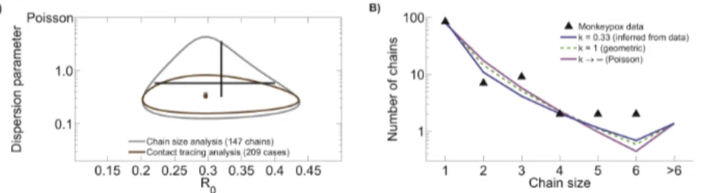
in the human population or by an increase in animal-to-human transmission. Since a relatively low incidence limits the data available for monkeypox (and many other subcritical diseases), it is helpful to determine how the type and quantity of data impacts the Figure 1. Contact tracing and chain size analysis of monkeypox data.A) Ninety percent confidence regions forR0andkinference are
shown for monkeypox data gathered between 1980 and 1984 in the Democratic Republic of Congo [26,27]. The two confidence regions are based on the same set of data. The chain size analysis is based on the number of cases in isolated outbreaks of monkeypox, whereas the contact tracing data are based on the number of transmission events caused by each case. The black cross hairs indicate the previously reported 90% confidence intervals for monkeypox transmission parameters based on the first generation of transmission in this data set [R0~0:32(0:22{0:40),k~0:58(0:32{3:57)]
[24]. B) Model predictions for the chain size distribution based on three different values ofk, including the ML value ofkthat is based on contact tracing data. A subset of the chain size data consisting of only those chains having exactly one identified primary infection is shown for comparison to model predictions. When the two-parameter ML value for the contact tracing data is compared to the likelihoods of thek~1andk??models, theDAICscores for the latter models are 4.3 and 23.3 respectively.
doi:10.1371/journal.pcbi.1002993.g001
Table 1.Inference results for monkeypox data.
R0 k
ML value for chain size analysis 0.30 0.36
90% CI for chain size analysis 0.22–0.40 0.16–1.47
95% CI for chain size analysis 0.21–0.42 0.14–2.57
ML value for contact tracing analysis 0.30 0.33 90% CI for contact tracing analysis 0.22–0.40 0.19–0.64
95% CI for contact tracing analysis 0.21–0.42 0.17–0.75
ability to detect a specific change inR0. Utilizing the results ofR0
andkinference for monkeypox in the 1980s, we can ascertain how the power to detect a statistically significant change inR0 varies
with the size of the data set and the magnitude of the change inR0
(figure 2A). As expected, the more data that are available, the more statistical power there is to detect a change in R0. The
sensitivity of chain size analysis for detecting a change in R0 is
almost identical to that of contact tracing analysis (when allowing kto be a free parameter in both analyses). This suggests that when faced with a trade-off, monitoring of R0 is enhanced more by
obtaining additional data on chain sizes (provided the sizes are accurately assessed) than by obtaining detailed contact tracing on a subset of available data.
Equally as important as detecting a change inR0 is knowing
when there may be an inaccurate report of a change. In the case of monkeypox, we find that assuming an incorrect level of transmission heterogeneity in a chain size analysis can lead to over-confident detection of a change in R0 relative to the 1980s
data. This is because under-estimating the degree of transmission heterogeneity leads to inappropriately narrow confidence intervals for the estimatedR0. Over-confident detection of a change inR0is
most worrisome when two data sets simulated using identical parameters give rise to distinct estimates ofR0 more often than
expected (table 2). This over-confidence arising from incorrect assumptions about k can also lead to a lack of specificity for detecting a change inR0 in simulated data sets, when inference
based on lettingkbe a free parameter is used as the gold standard (figure 2B). While it could initially appear preferable that incorrect kvalues can lead to greater probabilities of detecting changes in R0, this trades off against the higher rate of false positive detections
and a general loss of statistical integrity (e.g. the coverage of confidence intervals will not match the nominal levels).
Chain size thresholds provide an alternative approach to detecting change inR0
For many surveillance systems, large chains are more likely to be detected than isolated cases. This could give rise to biases in the chain size distribution data, which we address in a later section. In these situations, an alternative approach to detecting a change in R0 is to determine the size of the largest chain that would be
expected by chance (for some arbitrary threshold in the cumulative probability distribution) [2]. The size cutoff for what is then considered an anomalously large chain depends on the values of
bothR0andk(figure 3). As the assumed value ofkdecreases, the
chain size that is considered anomalously large will rise because superspreading events become more frequent. If chain size probabilities are calculated using traditional assumptions ofk~1 ork??, then too many false alarms may be raised concerning the number of chains that are perceived to be anomalously large, particularly for pathogens that exhibit significant transmission heterogeneity. The determination of a chain size cutoff also depends on whether the detection of large chains is based on individual reports versus the investigation of the largest chains in a collection of surveillance data (compare figures 3A and 3B).
In some situations, a rapid response protocol might be instituted to quickly investigate worrisomely large chains. In this case, an anomalous size cutoff can be chosen based on there being real-time reports of the size of single chains (as distinct from considering the largest chain obtained from an entire surveillance data set). However, assuming an incorrect value ofkcould trigger many false alarms for chains that are actually consistent with known transmission patterns (table 3). For instance if we assume that monkeypox transmission follows the parameters estimated with our ML model (blue line of figure 1B), then for a 99.9% cumulative distribution threshold settingk??will result in five-fold more chain investigations than ifkis set at the ML value of k~0:33.
In other situations, chain sizes may be evaluated collectively after a predefined period of surveillance. For the ML values ofR0
and k estimated for monkeypox in the 1980s, the cumulative distribution of chain sizes shows that there is a 95% chance that the largest of 100 observed chains will be less than 17 cases and a 99.9% chance that the chains will all be less than 31 cases. These results suggest cutoffs for chain sizes that deserve increased investigation (17 cases) and provides a chain size cutoff for determining when R0 has almost certainly increased (31 cases).
This contrasts with the 95% and 99.9% chain size cutoffs of 10 and 16 obtained whenk??is assumed.
Characterizing maximum likelihood inference ofR0 and kfrom chain size distributions
By demonstrating the concordance of results based on chain size and contract tracing data when inferringR0andk, our analysis of
monkeypox data provides motivation to further characterize the performance of inference based on chain size data. To evaluate the accuracy and precision of ML inference ofR0and kfrom chain
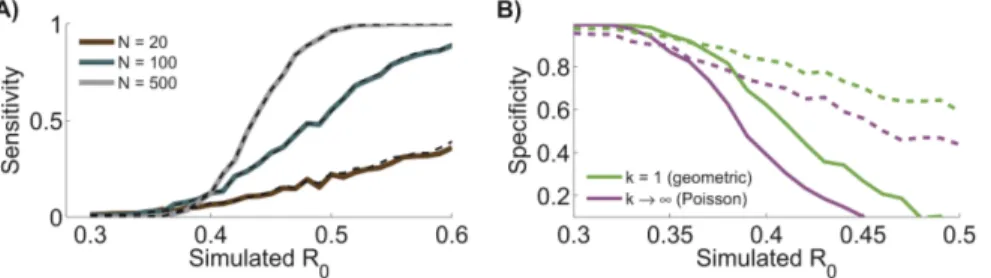
Figure 2. Chain size analysis clarifies surveillance needs.A) Applying maximum likelihood estimation to simulated data shows the sensitivity of chain size analysis and contact tracing analysis for detecting a change inR0. Results show the probability of detecting a significant change
between the monkeypox data from the 1980s and a simulated data set withk~0:33(equal to the ML value for the 1980s data) andR0specified along the x-axis. Statistical significance was determined by setting a 95% confidence threshold on the likelihood ratio test (details provided in methods section). Curves represent different values for the number of simulated chains,N. Results are depicted for inference from detailed contact tracing data (dashed line) or more readily available chain size data (solid line). B) The specificity for detecting a statistically significant change inR0(as
compared to 1980s monkeypox contact tracing data) is shown when various values ofkare assumed during chain size analysis (as applied to the same chain size data simulated for panel A). The specificity is defined as the probability that a change is not detected for an assumed value ofk conditioned on our gold standard for a lack of change (e.g. a change is not detected whenkis allowed to be a free parameter during inference). The solid line corresponds toN~500chains and the dashed line toN~100.
size data, we ran simulations for various combinations ofR0, k,
and number of observed transmission chains, N. For each simulated dataset, we determined the ML R0 and k values
(equations 9, 11 and 12) and evaluated whether the realized coverage probability of the 90% confidence intervals conformed to expectations (equations 22).
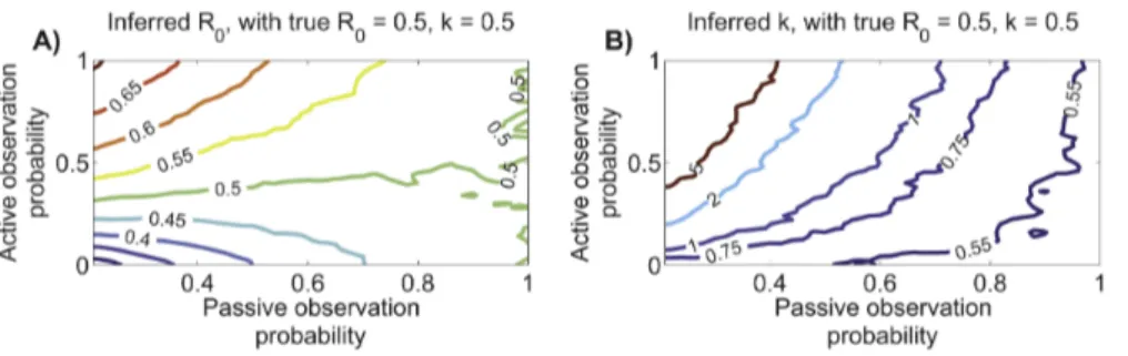
Due to the challenges of illustrating the dependence of inference error on three variables, this section considers two special cases of parameter values. First we fix N~100 and consider how the inference error depends onR0andk(figure 4 - left column). This
provides an assessment of error bounds when a realistic amount of data is available and when there is no prior information onR0or
k. Next we fix k~0:5 and consider how the inference error depends on R0 and N (figure 4 - right column). This scenario
highlights the relationship between inference accuracy and data set size when a significant amount of transmission heterogeneity is present. Qualitatively similar results are obtained when fixing different values forN ork(data not shown).
We limit our simulation results toR0§0:1because whenR0is close to zero there are too few secondary infections for inference to be meaningful. We also limit ourselves toR0ƒ0:9because large stuttering chain sizes become increasingly likely when R0
approaches one, and so our modeling assumption that transmis-sion is independent of stuttering chain size becomes increasingly dubious. Consistent with the range of inferred k from prior analysis of a variety of infectious diseases, we restrict our analysis to k§0:1 [24]. Meanwhile, we focus on kƒ10 since kw10 is similar to the Poisson distribution limit ofk??[29]. Lastly, we choose a range of 10 to 1000 forN since this reflects the size of most empirical data sets.
Inference of R0 from chain size distributions exhibits
little bias. We summarized the error inR0inference using the
root mean square of the relative and absolute errors,ar and aa
(equations 14 and 15). The relative error ar increases as R0
decreases, owing to the smaller denominator, andaralso increases
as k decreases because of increased variation arising from stochasticity as the offspring distribution becomes more skewed (figure 4A - left column). Meanwhile since ML inference is asymptotically unbiased,ardecreases as the data set size increases
(figure 4A - right column).
As with relative error, the absolute error aa increases as k
decreases. In contrast to ar, the dependence of aa on R0 is
relatively weak for high values ofkandN(figure 4B). However, if significant heterogeneity is present or when the data set is small, thenaagrows asR0increases. As with relative error,aatends to
zero for large data sets.
To further our understanding of the error inR0 inference, we
computed the bias and standard deviation arising in ML inference of R0. The former is a measure of accuracy and is potentially
correctable, while the latter is representative of imprecision inherent in stochastic processes and is uncorrectable. The bias of ML inference ofR0(figure 4C) is due to discrepancy between the
observed and predicted average chain size. The bias is always negative due to the non-linearity of equation 12, which makesR0
inference more sensitive to underestimates of the average chain size than to overestimates. The amplification of bias seen with decreasing k arises because greater transmission heterogeneity tends to produce chains that are either very small or very large, thus accentuating the influence of Jensen’s inequality on equation 12. Similarly, the magnitude of the bias increases for small N
Table 2.Probability of falsely detecting a change inR0.
Number of chains simulated Percentage whenkinferred Percentage whenk~1
Percentage whenk??
20 1.7 10.2 14.9
100 5.0 10.8 15.5
500 5.1 10.8 15.7
As detailed in the methods section, a statistical difference was determined by using the likelihood ratio test to compare two transmission models. The first model assigns separate values ofR0to the 1980s monkeypox data and the simulated data, while the second model assigns a singleR0to both data sets. Both models assign a single value ofkto both data sets. Since the second model is nested in the first, statistical significance was determined by setting a 95% confidence threshold on the likelihood ratio test. Probability values that exceed 5% indicate an over-abundance of false positive detections of change inR0. Each result was based on 10,000 simulations.
doi:10.1371/journal.pcbi.1002993.t002
Figure 3. Size of anomalously large chains.A) Size of an observed chain that is anomalously large as a function ofR0andk. The cumulative
because the stochastic nature of small data sets results in a larger sampling variance of the observed average chain size.
In principle, bias-correction could be applied toR0 inference.
However, this would be hard to do in a self-consistent manner because the bias depends on R0. To decide whether the extra
effort is worthwhile, it is instructive to know the fraction r by which aa would decrease if bias were eliminated (equation 18).
This fraction increases asR0increases,kdecreases, orNdecreases
(figure 4D). Howeverrremains less than0:1for a large region of parameter space. Therefore, given other uncertainties in data acquisition and analysis, it seems that bias correction will rarely be worthwhile.
Transmission heterogeneity can also be reliably inferred
from chain size distributions. Assessing inference of
transmis-sion heterogeneity is complicated by the inverse relationship betweenkand the variance of the offspring distribution. Thus we
measure the error ofkestimation in relation to1
k(equation 16). This emulates earlier work on ML estimation ofk, both as a general biostatistical problem and from contact tracing data [29,30]. In broad terms, the error of estimatingk from chain size data (ak)
decreases as R0 and N increase (figures 5A and 5B). This is
explained by there being more observed transmission events that provide information on transmission patterns. Meanwhile, the error tends to increase with decreasingk. This is likely due to a need for relatively large sample sizes to observe the rare superspreading events that are characteristic of lowkvalues [29]. Some caution is
needed in interpreting this trend because our error metric of 1 k increases as heterogeneity increases. However it is unlikely that this trend is an artifact of our chosen metric because it is also seen when other error metrics are used, such as the difference between the inferred and true coefficient of variation (data not shown).
Table 3.Frequency of anomalously large chains.
Cumulative distribution threshold k~0
:33assumed k~1assumed k??assumed
95% 4.9% (§3cases) 4.9% (§3cases) 4.9% (§3cases)
99% 0.88% (§7cases) 1.29% (§6cases) 1.94% (§5cases)
99.9% 0.09% (§14cases) 0.22% (§11cases) 0.43% (§9cases)
The cutoff for a chain sizes that are considered anomalously large was determined by when the cumulative chain size probability exceed the cumulative distribution threshold forR0~:30(ML value for 1980s monkeypox data) andkas indicated in the table. The frequency of outlier detection was then determined according to the probability that chain sizes would exceed the chain size cutoff as predicted by the ML values ofR0~:30andk~0:33for monkeypox.
doi:10.1371/journal.pcbi.1002993.t003
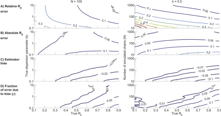
Figure 4. Characterization ofR0inference as a function ofR0andkwithN~100(left column) and as a function ofR0andNwith k~0:5(right column).The axes represent the trueR0,kandNinputs for the simulations. A) Root mean square relative error for ML inference ofR0
(ar). B) Root mean square absolute error for ML inference ofR0(aa). C) Bias ofR0inference (d). D) Fraction of theR0absolute error that is attributable
to bias (r). The contour plots were generated based on a lattice of simulation results for linearly spaced values ofR0and logarithmically spaced
values ofkorN. The values for each lattice point were computed by averaging the results of 2,000 simulations. For visualization purposes, simulation results were smoothed by a one-neighbor moving average.
Because of the non-intuitive relationship between ak and
confidence intervals for k, we have illustrated the performance ofkinference for four specific choices ofR0andN (figures 5C–
5F). These plots reinforce the trends seen in panels A and B. In particular, narrower and more consistent confidence intervals for largeN and largeR0 support the conclusion that this region of
parameter space allows the most precise and accurate inference of k. The confidence intervals are also narrower for smaller k. However, this does not accurately reflect the uncertainty in the degree of transmission heterogeneity because small changes in small values of k can significantly change the offspring distribu-tion’s coefficient of variation. In contrast, the more rugged curves for ML inference when kw1 should be interpreted with consideration of the offspring distribution changing minimally for higher values ofk. Despite the inherent difficulties of inferring low values ofk, the ML approach appears robust because there is no discernible bias of the ML estimate of k and the median confidence intervals consistently include the true values ofk.
Motivated by the observation that the ML estimator forR0is a
simple function of the average chain size, we explored whether accurate inference forkcan be obtained by considering just the first two moments of the chain size distribution (equation 7, figures 5C–5F). Second moment inference improves as N increases, but there is a clear bias towards over-estimation ofk. The non-negligible bias suggests that whenever possible it is preferable to estimatekby ML inference from the full distribution of chain sizes.
Confidence intervals show accurate coverage. Since
confidence interval calculations are independent of the particular metric used for quantifying inference error (e.g. insensitive to our
use of1
kfor our error metric), their coverage accuracy provides a useful assessment of ML inference [31]. For most of theN~100 andk~0:5parameter space slices, the 90% coverage probability ofR0estimates varied from 88% to 93% and tended to increase
with increasingk (data not shown). This coverage probability is
consistent with the expected value of 90%. The one exception was fork~0:5, Nv20 and R0v0:5when the coverage probability rose as high as 98%. This occurred because confidence intervals got wider for these small data sets, and not becauseR0inference
was more precise. The coverage probabilities for confidence intervals ofkestimates show similar concordance. As with theR0
estimates, whenR0andNare both low, the coverage probability
forktended to be higher than the nominal level of 90%. It was also too high whenkapproached higher values, but this is likely due to the boundary effects whenk??. The take-home message is that for most of parameter space, the confidence intervals forR0
andkinference can be trusted when ML inference is applied to high quality data.
Overall, our characterization of the inference ofR0andkfrom
the size distribution of stuttering chains shows that estimation accuracy is more likely to be limited by data or shortcomings of our modeling assumptions than by biased inference. For simulated data over a wide range of parameter values, inference ofR0has an
error of less than 10%, negligible bias and reliable confidence intervals. Inference ofkalso has reliable confidence intervals, but unlikeR0, the parameter itself is typically not the direct focus of
epidemiological interest. Thus caution is needed in interpreting the absolute error inkestimates, due to the nonlinear relationship betweenkand the coefficient of variation and other measures of heterogeneity for the offspring distribution.
Data limitations have variable impact on inference results The preceding analyses have shown the potential for accurate inference of transmission parameters from chain size data, but we have not yet considered how imperfect case detection impacts inference results. We have also ignored complications arising when multiple chains are mixed into a single cluster. This latter scenario allows the possibility that some primary infections are falsely classified as secondary cases. Here we consider whether and how these types of data limitations impact inference results.
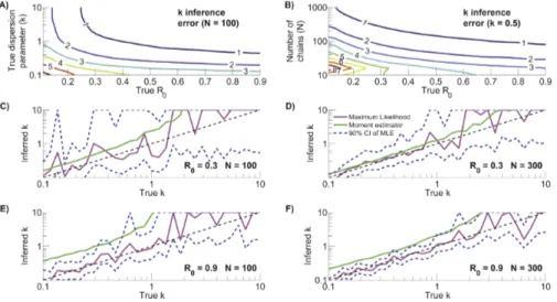
Figure 5. Characterization ofkinference.A) Error ofkinference as quantified by the root mean square of the absolute differences between the reciprocals of the inferred and true value ofkfor simulated data (ak). The contour plot was generated based on the same simulations and inference
procedure that was used to produce theN~100panels of figure 4. B) Same as panel A except thatk~0:5for all simulations and now the number of simulated chains varies. C) Summary of how wellkinference works whenR0~0:3andN~100. The dashed black line represents a perfect match
between the true and inferredkvalues. The magenta line shows the median value of ML inference ofk. The dashed blue lines show the median values of the upper and lower limits of the 90% confidence intervals fork. For visualization purposes and becausekw10is essentially a Poisson distribution, the upper confidence intervals were bounded atk~10. The green line shows the median estimate forkinference based solely on the first and second moments of the simulated data,^kkh (equation 7). All curves were determined from the results of one thousand simulations for logarithmically distributed values of the truek. D–F) Same as panel C, but for differentR0andNpairs.
The bias arising from imperfect observation depends on
which cases are unobserved. No surveillance system is perfect
and some cases will be missed. However the mechanisms underlying imperfect observation can alter R0 estimation in
different ways [2]. For instance, if the observation of each case is independent of all other cases, then the average observed size of a chain will be smaller and the resultingR0estimates will be smaller.
However, other processes such as retrospective investigation can paradoxically increase the average observed chain size and thus lead to higher estimates ofR0.
By modeling observation as a two-step process, we can explore the impact of a diverse range of scenarios. We define the passive observation probability as the probability that any case will be detected by routine surveillance measures. This probability applies independently to all cases, so multiple cases in the same chain can be detected by passive surveillance. In some settings, there is an active surveillance program that investigates outbreaks that have been detected by the passive system. We define the active observation probability as the probability that a case will be detected by active surveillance, conditional on that case not having been detected by passive surveillance. Cases can be detected by active surveillance only if they belong to a transmission chain where at least one case is detected by passive surveillance. (When the active observation probability is zero or one, respectively, our observation model maps onto the ‘random ascertainment’ and ‘random ascertainment with retrospective identification’ scenarios previously analyzed [2].).
When the passive observation probability approaches one, essentially all cases are observed and so the inferredR0andkare
close to their true value (figure 6). If the passive observation probability is less than one and the active observation probability is low, the average observed size of chains is smaller than the true value, and theR0tends to be under-estimated (figure 6A). When
the passive observation probability is low but the active observation probability is high, there is a tendency to observe most cases in most of the large chains but to miss many of the small chains entirely. This leads to over-estimation ofR0.
Imperfect observation tends to cause over-estimation of k, particularly when the passive observation probability is low and the active observation probability is high (figure 6B). This trend arises because the observed fraction of chains that are isolated cases is likely to be under-estimated. Since a high proportion of isolated cases is a hallmark of transmission heterogeneity, inference from data that under-represent isolated cases will be biased toward homogeneity. This implies that when chain size analysis suggests thatkv1(such as with the 1980s monkeypox data), the conclusion is likely to be a true reflection of heterogeneous transmission dynamics. In contrast, if initial data analysis suggests that transmission is relatively homogeneous, then the possibility that the analysis is impacted by imperfect observation of cases should be considered.
Overall, our observation model suggests that inference of R0
andkis relatively robust when at least eighty percent of cases are observed. Due to the extensive resources provided for monkeypox surveillance in the 1980s [1], this is likely to have been true for the monkeypox data set we have analyzed. However this level of case detection is unlikely to be attainable for many surveillance programs. An important direction for further work is to correct for imperfect data by incorporating the observation process into the inference framework.
Accurate assignment of primary infections is more
important than disentangling infection clusters. A key
challenge of analyzing chain size data for monkeypox and many other zoonoses is that primary infections are typically clinically
indistinguishable from secondary infections. Yet each type of infection represents a distinct transmission process and ignoring this distinction can skew epidemiological assessments. In the context of chain size distributions, this causes a problem because multiple chains can be combined into one cluster. To improve our understanding of how inference ofR0andk is impacted by how
these entangled transmission chains are handled, we compared our initial analysis of monkeypox data to three alternative approaches. The monkeypox dataset we analyze groups cases in terms of infection clusters rather than transmission chains. Our primary strategy to cope with this limitation was to consider all possible ways that the ambiguous infection clusters could be divided into chains (what we term the combinatorial approach). This effort was greatly facilitated by knowing how many primary cases were present in each infection cluster. We now consider the importance for transmission parameter inference of identifying primary cases correctly. We then consider the additional value of more detailed contact tracing data that allows disentanglement of clusters into individual chains.
To assess how clusters identified as having multiple primary infections (equivalent to the presence of ‘co-primary infections’) impactR0andkinference, we performed ML inference when the
22 co-primary classifications were ignored and all 125 clusters were treated as single transmission chains (see ‘simple cluster analysis’ in figure 7). The inferred value ofR0(and its confidence
interval) was higher than our original estimate, because ignoring primary infections leads to underestimation of the number of chains, which in turn leads to an increase in the observed average chain size. Further, in contrast to our initial results, the confidence interval for k suggests that transmission is unlikely to be more heterogeneous than a geometric distribution. This change arises because treating clusters with co-primary cases as single chains will deflate the apparent frequency of isolated cases, which is a key indicator of transmission heterogeneity.
To determine the importance of disentangling transmission chains fully before performing inference, we considered two methods for dividing infection clusters with multiple primary infections into individual transmission chains (figure 7). Our heterogeneous assignment maximizes the number of isolated cases and thus produces more chains of relatively large size, while the homogeneous assignment minimizes the number of isolated cases and thus produces a higher proportion of intermediate sized chains. The average chain size and corresponding ML estimates of R0are identical (per equation 12), but the confidence intervals for
R0 differ slightly depending on the inferred k values. Not
surprisingly, when clusters are divided as evenly as possible into chains, the ML estimate ofkand confidence interval are higher than when clusters are divided in a way that maximizes the number of isolated cases. The ML value based on our initial combinatorial approach (figure 1 and table 1) falls between the ML values obtained using the two assignment procedures. This supports the intuitive conclusion that the true chain assignment is likely a mix of the two extreme assignment algorithms considered. Only 5 of the 19 clusters containing multiple primary infections had ambiguity with regard to the size of constituent chains. Thus the noticeable difference between the ML estimates ofk for the homogeneous and heterogeneous chain assignments underscores how the inference ofk is sensitive to details of infection source assignments. However, the relatively compact confidence region for the combinatorial approach suggests that, in many circum-stances, it may not be necessary to disentangle all overlapping transmission chains. In fact, as the homogeneous chain assignment shows, there is a risk thatad hoc disentanglement of chains may
combinatorial approach to be reliable, it is essential to identify how many cases in each cluster are due to primary infection.
Overall, our analysis of monkeypox data highlights how inference of transmission parameters from chain size data can be complicated when infection clusters may contain multiple primary infections. More generally, the challenge of properly differentiat-ing primary from secondary infections is of fundamental impor-tance for analysis of stuttering zoonoses. Even when well-trained surveillance teams are on site to assess transmission pathways, it may be impossible for them to decide between two equally likely infection sources. For instance, it can be difficult to decide if a mother contracted monkeypox because she cared for an infected child or because she contacted infected meat (in the same contact event as the child, or a later one). The theory presented here forms a foundation for further research on infection source assignment and its relationship to underlying transmission mechanisms. Future investigations can leverage existing methods of source assignment developed for supercritical diseases, which utilize various epidemiological data such as symptom onset time, risk factor identification and pathogen genetic sequence data [32–34]. These types of theoretical developments, combined with strong collaborative ties between field epidemiologists and modelers,
would likely expand the use of existing epidemiological data and improve resource allocation for future surveillance efforts.
Model limitations
Several of our modeling assumptions deserve further explora-tion. In particular, the assumption that transmission can be described by independent and identical draws from a negative binomial offspring distribution is a simplification of some forms of transmission heterogeneity. For example, if heterogeneity is driven largely by population structure, such that susceptibility and infectiousness are correlated, then the relation between R0 and
heterogeneity can differ from what is represented in our model [35]. Specific scenarios that can give rise to such correlations include the existence of clustered pockets of susceptible individuals, impacts of coinfection or immunosuppressive conditions, or transmission heterogeneity that arises chiefly from variation in contact rates rather than variation in the amount of virus shed [36–38]. This issue is especially relevant for preventable diseases such as measles, because large outbreaks in developed countries are often associated with particular communities in which vaccine refusal is common [16,39]. Local depletion of susceptible individuals, which can even occur within a household, can also Figure 6. Influence of imperfect observation onR0 andkinference.A) The inferred value of R0 is plotted as a function of the two
probabilities we use to model surveillance. Results are based on a simulation of 10,000 chains for a lattice ofR0 andkpairs. For visualization
purposes, simulation results were smoothed by a one-neighbor moving average. B) Analogous to panel A but for the dispersion parameter. doi:10.1371/journal.pcbi.1002993.g006
Figure 7. Complications of entangled chains can affect inference.ML estimates ofR0andkand corresponding 90% confidence regions are
when all clusters are treated as chains, and for two approaches to assigning constituent chain sizes for clusters with more than one primary case (details provided in the text). For visual comparison, the contour corresponding to the chain size analysis from figure 1 is replicated.
impact the estimation ofR0andk. By diminishing the possibility
of large outbreaks, the depletion of a susceptible population is likely to decrease estimates ofR0and increase estimates ofk. We
hope that our use of a likelihood function that combinesR0and
transmission heterogeneity will facilitate future work that addresses these modeling challenges in a self-consistent manner.
Conclusion
Data acquisition is often the limiting factor for assessing the transmission of subcritical diseases that pose a threat of emergence. Our findings can assist future surveillance planning by drawing attention to the utility of chain size data when contact tracing data are too difficult to obtain. We have shown that both R0and the degree of transmission heterogeneity can be inferred
from chain size data, and have demonstrated that chain size data can give equivalent power to contact tracing data when deciding if R0 has changed over time. In fact, even knowledge of the
largest chain size alone can be helpful for monitoring change in R0, provided that the degree of transmission heterogeneity has
been reliably measured. Conversely, we have demonstrated that inaccurate assumptions about transmission heterogeneity can lead to errors in R0 estimates and possible false alarms about
increased transmission. We have also found that inference can be accomplished when transmission chains are entangled into infection clusters, provided that the number of primary infections in each cluster is known. For the particular case of human monkeypox, our findings support previous analyses that have identified substantial transmission heterogeneity, but conclude that endemic spread would only be possible if there is significant demographic change or viral adaptation to enable greater human-to-human transmissibility. Since a mechanistic under-standing of transmission dynamics is important for quantifying the risk of emerging diseases and predicting the impact of control interventions, we hope our findings will assist in providing robust epidemiological assessments for relevant public health decision-making.
Methods
Monkeypox data
We analyzed previously reported data describing monkeypox cases identified between 1980–1984 in the Democratic Republic of Congo (formerly Zaire) [1]. These data were collected in order to assess the potential of monkeypox to emerge as an endemic human pathogen in the wake of smallpox eradication. Contact tracing and subsequent analysis by epidemiological teams classified each identified cases as a primary case, arising from animal-to-human transmission, or a secondary case, arising from human-to-human transmission. The data set consists of 125 infection clusters [26,27]. Most clusters contained just one primary case and thus constituted a single transmission chain. However nineteen of the clusters had overlapping transmission chains, because contact tracing revealed they contained more than one primary case.
The raw cluster data for monkeypox was obtained from table 1 of [26]. Our baseline inference of transmission parameters is based on considering all the possible ways this cluster data can be separated into individual transmission chains. To explore the specific impact of entangled transmission chains on the inference of transmission parameters, we also investigated the impact of three approaches of using the cluster size data to assign an explicit chain size distribution (table 4). In the ‘simple cluster analysis’ approach, we treat all clusters as though they were a complete stuttering chain and ignore the complications of multiple primary infections. The other two approaches use different algorithms to
divide the clusters that have multiple primary infections into constituent chains. In our ‘homogeneous assignment’ distribution, clusters were divided as evenly as possible. For example, a cluster of total size four with two co-primary cases is tabulated as two chains of size two. Meanwhile, our ‘heterogeneous assignment’ distribution maximized the number of isolated case counts when disentangling clusters. For this distribution, a cluster of size four with two co-primaries is tabulated as a chain of size one and a chain of size three.
Offspring distribution
We analyze the transmission dynamics of stuttering chains using the theory of branching process [22,40,41]. The key component of this theory is the probability generating function,Q(s)~P?
i~0qisi
of the offspring distribution. This function describes the probabil-ity distribution for the number of new infections that will be caused by each infected case. The probability that an infected individual directly causesiinfections isqi, and hence the probability that an
individual is a dead-end for transmission is q0. Subject to the
standard assumption that transmission events are independent and identically distributed,Q(s)contains all the information needed to determine the size distribution of stuttering chains.
The choice of offspring distribution is important because it defines the relationship between the intensity and heterogeneity of transmission. We adopt a flexible framework by assuming secondary transmission can be characterized by a negative binomial distribution with meanR0and dispersion parameter k.
The corresponding generating function, valid for all positive real values ofR0andk, is [24]
Q(s)~ 1zR0 k (1{s)
{k
: ð1Þ
A key advantage of using a two-parameter distribution over a one-parameter distribution (such as the geometric or Poisson distribution) is that modulating k permits the variance to mean
ratio,1zR0
k, to range from one to?without any change inR0. Further, the geometric and Poisson distributions are conveniently nested cases of the negative binomial distribution whenk~1and k??respectively.
Simulations
All simulated chains start with a single primary infection. Then the number of first generation cases is decided by choosing a random number of secondary cases according to a negative binomial distribution with meanR0and dispersion parameter k.
For each case in the first generation (if any exist), a new random number is chosen to determine how many consequent second generation cases there are. This is repeated until the stuttering chain goes extinct. Since our focus is on R0v1, all simulated
chains eventually go extinct. Simulated contact tracing data consisted of the individual transmission events that produce simulated chain size data.
To simulate imperfect observation, we first simulated a set of true transmission chains, then simulated whether each case would be observed according to the passive observation probability. Finally, for chains where at least one case was detected passively, we simulated which additional cases were observed according to the active observation probability.
Stuttering chain statistics
The next two subsections derive the average size and variance of the distribution. As a by-product, we obtain a first order moment estimator forR0and a second order moment estimator fork. We
will see that the first order moment estimator of R0 exactly
matches the ML value of R0. This finding provides a simple
relationship between observed data andR0inference.
Average size of stuttering chains. Since the average
number of cases per generation declines in a geometric series when R0v1, the average stuttering chain size, m, is simply
[21,41,42]
m~X
?
i~0
Ri 0~
1 1{R0:
ð2Þ
This relationship can be inverted to obtain the first moment estimator forR0based on the observed mean chain size,mm,
^ R R0~1{
1 m
m: ð3Þ
An alternative expression forRR^0can be obtained for a data set
encompassing numerous chains by lettingNpand Nsdenote the
number of primary and secondary cases, respectively. Then since Npis the total number of chains andNpzNsis the total number
of cases,mm~Np zNs
Np
. Therefore,
^ R R0~1{
Np
NpzNs
~ Ns NpzNs
ð4Þ
which is the fraction of all observed cases due to secondary transmission, as noted previously [21].
Coefficient of variance for the offspring and chain size
distributions. The coefficient of variation (COV) provides
quantitative perspective on the relationship between k and observation of cases. The variance of the negative binomial
distribution is given bys2
nb~R0:(1z R0
k ). Therefore the COV for the offspring distribution,snb
R0
, is
hoff~
ffiffiffiffiffiffiffiffiffiffiffiffiffiffiffi
1 R0
z1 k
s
: ð5Þ
Meanwhile, branching process theory shows that the variance of
the chain size distribution is s
2 nb
(1{R0)3
when R0v1 [41,42].
Therefore the COV for the chain size distribution is,
hcsd~
ffiffiffiffiffiffiffiffiffiffiffiffiffiffiffiffiffiffiffiffiffiffiffiffiffiffi s2
nb
(1{R0)3 :
1
m2 s
~
ffiffiffiffiffiffiffiffiffiffiffiffiffiffiffiffiffiffiffiffiffiffiffiffi
R0:(1z R0
k )
1{R0 s
: ð6Þ
The COV of the negative binomial offspring distribution increases as k decreases (figure 8A), reflecting the rise in transmission heterogeneity [24,43]. The COV of the chain size distribution also increases askdecreases (equation 6, figure 8B). In contrast to the COV of the offspring distribution, for a given value of k, the COV of the chain size distribution increases as R0
increases. This is due to stochastic variation, which gets amplified for longer chains asR0rises.
Equation 6 can be inverted to obtain a second moment estimator forkbased on the observed coefficient of variation,hhcsd,
and the inferredRR^0,
^ k kh~
^ R R2
0 h
h2csd:(1{RR^0){RR^0
: ð7Þ
The 2nd moment estimator of k does not always provide valid inference ofkbecause the denominator can be negative. Because this circumstance arises when the chain size variance is particularly small, we interpret it as corresponding to a Poisson offspring distribution since this is the most homogeneous distribution allowed by the negative binomial model.
Size distribution of stuttering chains
Beyond determining the relationship betweenR0,k,mandhcsd,
our assumptions about the transmission process allow us to use branching process theory to characterize the complete size distribution of stuttering chains [23,40–42]. Let rj be the
probability of a transmission chain having overall size j. If one
Table 4.The number of transmission chains tabulated by size (i.e. total number of cases) for three different assignment algorithms.
Chain size Simple cluster analysis homogeneous assignment heterogeneous assignment
1 84 114 120
2 19 16 7
3 11 11 12
4 5 2 3
5 2 2 3
6 4 2 2
definesTj(s)~
1 j½Q(s)
j
, then [44],
rj~
1 (j{1)!T
(j{1)
j Ds~0 ð8Þ
whereT(j{1)
j is the(j{1)th derivative ofTj. See the supporting
text (Text S1) for a derivation of this formula that develops intuition for the specific application to disease transmission. In particular, the supporting text explains the validity of equation 8 for both R0v1 and R0w1, which extends recent findings of
Nishiura et al. [23].
Based on equation 1 the formulae forTj(s)andTj(i)are,
Tj(s)~
1 j: 1z
R0
k (1{s)
{kj
Tj(i)(s)~
P
i{1 z~0 (kjzz)
j
R0
k
i
1zR0 k (1{s)
{kj{i
where the latter formula was derived by induction. Substitution into equation 8 gives,
rj~
P
j{2 z~0 (kjzz)
j!
R0
k
(j{1)
1zR0 k
{kj{jz1 :
Noting that the Gamma functionC(x)satisfiesx~C(xz1) C(x) and thatx!~C(xz1)for integerx, we can rewrite the last formula as
rj~C
(kjzj{1) C(kj)C(jz1)
R0
k
j{1
1zR0 k
kjzj{1: ð9Þ
This equation matches the relation derived by Nishiura et al. for
the specific case ofR0w1[23]. This relationship was verified by
using a stochastic simulation model to simulate many stuttering chains as described above (data not shown).
Equation 9 forms the basis of interpreting chain size distribution data because it provides the probability that a randomly chosen stuttering chain has a size j. However, from the perspective of considering how chain size observations reflect overall disease burden, it is also helpful to consider the probability, wj, that a
randomly chosen case is in a stuttering chain of size j. This ‘weighted’ probability density is obtained by scaling eachrj byj
and then renormalizing. Accordingly,
wj~
1
m:j:rj~(1{R0):j:rj: ð10Þ
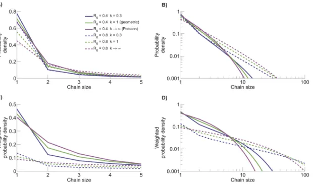
For a given value of R0, decreasingk leads to both a higher
number of isolated cases and a higher number of large stuttering chains (figure 9). Meanwhile, the homogeneous Poisson offspring distribution maintains the highest probabilities for intermediate sized stuttering chains (seen most clearly in figure 9D), Thus, branching process theory provides an analytical foundation for prior computational results showing that greater transmission heterogeneity results in a higher frequency of relatively large stuttering chains [24,25,29,43,45]. Of particular interest, the fraction of stuttering chains that consist of a single isolated case is substantial for all parameter sets considered. Meanwhile, the weighted probability density shows that the probability of a case occurring as an isolated case can be significantly less than the probability of a randomly chosen stuttering chain having size one.
Maximum likelihood estimation ofR0 andk
We employ maximum likelihood estimation for R0 and k
inference because it is asymptotically unbiased and maximally efficient (i.e. there is minimum sampling variance). To implement ML estimation forR0andkusing stuttering chain size distribution
data, we letN denote the total number of stuttering chains in a given dataset, andnj represent the number of chains with sizej.
Then the likelihood,L, of the data set is,
L~ P
?
j~1r nj
j : ð11Þ
The ML estimate ofR0andkis found by maximizing the
log-likelihood function with respect to both parameters. The
maximum occurs whend(lnL) dR0
~d(lnL)
dk ~0. Focusing on finding Figure 8. Coefficient of variation for offspring and chain size distribution.The COV for the offspring distribution (i.e. the distribution for the number of transmission events caused by each case, panel A) and chain size distribution (panel B) are both a function ofR0andk.
the ML estimate forR0, one finds,
d(lnL) dR0
~X
?
j~1
nj:d(ln rj) dR0
~X
?
j~1
nj: j{1
R0
{kjzj{1 kzR0
~ k
R0:(kzR0) X
?
j~1
nj:½j(1{R0){1:
Then since the total number of chains isN~P?j~1nj and the
observed average chain size ismm~1 N:
X? j~1nj:j,
d(lnL) dR0
~ kN R0:(kzR0)
m
m(1{R0){1
½ :
Solving ford(lnL) dR0
~0gives,
^ R
R0,MLE~1{
1 m
m ð12Þ
which is identical to the first moment estimator RR^0 given by
equation 2.
The ML calculation for the dispersion parameter, ^kk, is not analytically tractable andkk^depends onRR^0. Thus,kk^is obtained by
computational optimization of the log likelihood. Since the limits k??andk?0lead to convergence difficulties, we set lower and upper limits of 0.00001 and 1000 for^kk. This lower bound forkis well below the range needed to infer biologically relevant values of
kand the upper bound forkis essentially equivalent to a Poisson distribution. We cannot attempt k inference when a simulated data set has no secondary transmission (implying RR^0~0).
Therefore these data sets, which occasionally occur when both R0 and N are low, were discarded from our simulation-based
characterization ofkinference.
Combinatorial method for maximum likelihood
estimation of R0 and k for monkeypox clusters. As
mentioned, some of the monkeypox infection clusters could not be unambiguously divided into constituent chains. For our baseline ML inference of R0 and k (figure 1 and table 1), we
approach this ambiguity by considering all possibilities of chains that could give rise to clusters of the observed size. For instance, the probability that an infection cluster having two primary infections has an overall size of four is,
r1:r3zr2:r2zr3:r1 :
To conduct inference ofR0andkthese combinatorial terms were
included in the product of equation 11.
Contact tracing method for maximum likelihood
estimation of R0 and k for monkeypox. Contact tracing
investigations yield direct information about how many infections are caused by each infectious case. By analogy to equation 11, the likelihood of contact tracing data can be written as,
L~
P
?
i~0s mi
i ð13Þ
wheresiis the probability that a case will directly causeiinfections
andmiis the number of cases that directly causeiinfections. For
our model, si is the probability density of a negative binomial
distribution,
Figure 9. The size distribution of stuttering chains varies as a function ofR0andk.A) The probability distribution for chain sizes for various parameter choices, when transmission is described by a negative binomial offspring distribution. B) Same as panel A but with logarithmically scaled axes, to highlight lower frequencies and larger chain sizes. C) The weighted probability density for the sameR0andkpairs given in panel A. D) Same
si~ C
(izk) C(iz1)C(k)
k R0zk
k
r R0zk
i
:
Although full contact tracing data are unavailable for monkeypox in the 1980s, much of it can be reconstructed from the tabulation of monkeypox cases in which the number of cases is noted for each generation of each cluster (table 1 of [26]). As in the case of infection clusters with multiple primary infections, there is some ambiguity in the contact tracing data for 11 of the 209 cases when it is only known that a set of cases lead to one or more infections. However, it is straightforward to consider the probability for each of the possible combinations and incorporate their sum as a factor in equation 13. This combinatorial approach was used to create figure 1 and table 1.
Measuring the performance ofR0 andkinference To study the precision and accuracy of our ML approach, we simulated many data sets for a range of values ofR0,kandN. We
inferred the ML values ofR0andkfrom the simulated data, and
compared these values to the true values used in the simulation.
Error of R0 and k inference. We use two metrics to
summarize the error in inferred values ofR0. The first metric is the
root mean square relative error, defined as
ar~
ffiffiffiffiffiffiffiffiffiffiffiffiffiffiffiffiffiffiffiffiffiffiffiffiffiffiffiffiffiffiffiffiffiffiffiffiffiffiffiffiffiffiffiffiffiffiffiffiffiffiffi
lim
M??
1 M
XM
i~1 ^ R R0i{R0
R0 !2 v
u u
t ð14Þ
whereRR^0i is the ML value ofR0for a simulated datasetiwhich
had true parameter valuesR0,k andN. In practice, the limit is
taken to a reasonable number of simulations, M, based on convergence ofar(we typically setM~2000).
Another useful metric for characterizingR0inference is the root
mean square absolute error defined as
aa~
ffiffiffiffiffiffiffiffiffiffiffiffiffiffiffiffiffiffiffiffiffiffiffiffiffiffiffiffiffiffiffiffiffiffiffiffiffiffiffiffiffiffiffiffiffiffiffi
lim
M??
1 M
XM
i~1
(RR^0i{R0)2 v
u u t
: ð15Þ
Since the relative error scales withR0it can be particularly useful
in assessing the significance of small differences betweenR0values
when secondary transmission is quite weak. Meanwhile, as explained below, the absolute error is useful for decomposing the source of R0 measurement uncertainty into bias and
unavoidable stochastic randomness.
Since the coefficient of variation of the negative binomial
distribution is a function of1
k, the effect of changingkby a fixed amount is much greater whenk is small than whenk is large. Therefore we choose to measure the error as the difference in the reciprocals of the inferred and truek, because this leads to more consistent interpretation of inference results. The convention of using the reciprocal transform for inference onkis well established in the biostatistics literature on negative binomial inference [29,30]. We define the root mean square error ofkas,
ak~
ffiffiffiffiffiffiffiffiffiffiffiffiffiffiffiffiffiffiffiffiffiffiffiffiffiffiffiffiffiffiffiffiffiffiffiffiffiffiffiffiffiffiffiffiffiffi
lim
M??
1 M
XM
i~1
1 ^ k ki {1 k 2 v u u
t ð16Þ
where^kki is the ML estimate of k for theith dataset. Whenever ^
k
kiv0:05, it is replaced by 0.05 in this calculation to avoid numerical instabilities arising from small denominators. The threshold of 0.05 was chosen because it is close to, but below the observed range fork in infectious disease transmission data [24].
Bias ofR0 inference. The inference error for R0 contains
contributions from estimator bias and from the inherently random nature of the processes generating the data. The bias of R0
inference is given by
d~ lim
M??
1 M
XM
i~1 ^ R
R0i{R0 ð17Þ
for fixed R0, k and N. The contribution of randomness is
summarized by the standard deviation of the ML values ofR0
associated with a set of simulation parameters, sRR^
0. The two
sources of error add in quadrature to form the root mean square absolute error,
a2a~s2RR^ 0zd
2 :
If the bias were eliminated from theRR^0estimator, then the error
would simply besRR^
0. Therefore, the fractional reduction of the
absolute error inR0inference that would be possible with optimal
bias correction is
r~
aa{sRR^0 aa
~1{
sRR^ 0 aa :
ð18Þ
Confidence intervals. We use likelihood profiling to
deter-mine the confidence intervals for inferred values of R0. More
specifically, for a given dataset letL(R0,k) denote the likelihood
for particular values of the parameters R0 and k. Then define
L’(R0)~maxk[(0??)L(R0,k). In addition, let LL^ denote the
likelihood for the ML estimates ofR0andk. Then the endpoints
of the confidence interval corresponding to a confidence levelvare obtained by finding the two values ofR0that solve,
ln LL^ L’(R0)~
x2 1(v)
2 ð19Þ
where x21(v) denotes the inverse of the chi-square cumulative distribution function for one degree of freedom [31].
Our approach does not put any explicit constraints on the value of R0, but equation 12 will always produce a ML estimate
satisfying RR^0v1, implying that subcritical transmission is likely
when all observed chains are self-limited. However, ifR0exceeds
one and the number of observations is small, all observed chains may be self-limited due to stochastic extinction. Therefore,L’(R0)
is continuous across the critical value ofR0~1and the upper limit
of theR0confidence interval can exceed one.
To determine the associated confidence interval forkinference, we define L’(k)~maxR0[(0??)L(R0,k). Then the confidence
interval endpoints are the two values ofkthat solve
ln LL^ L’(k)~
x2 1(v)