ACPD
15, 21219–21269, 2015Parameterization of oceanic whitecap fraction based on satellite observations
M. F. M. A. Albert et al.
Title Page
Abstract Introduction
Conclusions References
Tables Figures
◭ ◮
◭ ◮
Back Close
Full Screen / Esc
Printer-friendly Version
Interactive Discussion
Discussion
P
a
per
|
Discussion
P
a
per
|
Discussion
P
a
per
|
Discussion
P
a
per
|
Atmos. Chem. Phys. Discuss., 15, 21219–21269, 2015 www.atmos-chem-phys-discuss.net/15/21219/2015/ doi:10.5194/acpd-15-21219-2015
© Author(s) 2015. CC Attribution 3.0 License.
This discussion paper is/has been under review for the journal Atmospheric Chemistry and Physics (ACP). Please refer to the corresponding final paper in ACP if available.
Parameterization of oceanic whitecap
fraction based on satellite observations
M. F. M. A. Albert1, M. D. Anguelova2, A. M. M. Manders1, M. Schaap1, and
G. de Leeuw1,3,4
1
TNO, P.O. Box 80015, 3508 TA Utrecht, the Netherlands
2
Remote Sensing Division, Naval Research Laboratory, Washington, DC 20375, USA
3
Climate Research Unit, Finnish Meteorological Institute, Helsinki, Finland
4
Department of Physics, University of Helsinki, Helsinki, Finland
Received: 30 May 2015 – Accepted: 3 July 2015 – Published: 6 August 2015 Correspondence to: M. F. M. A. Albert ([email protected])
ACPD
15, 21219–21269, 2015Parameterization of oceanic whitecap fraction based on satellite observations
M. F. M. A. Albert et al.
Title Page
Abstract Introduction
Conclusions References
Tables Figures
◭ ◮
◭ ◮
Back Close
Full Screen / Esc
Printer-friendly Version
Interactive Discussion
Discussion
P
a
per
|
Discussion
P
a
per
|
Discussion
P
a
per
|
Discussion
P
a
per
|
Abstract
In this study the utility of satellite-based whitecap fraction (W) values for the prediction of sea spray aerosol (SSA) emission rates is explored. More specifically, the study is aimed at improving the accuracy of the sea spray source function (SSSF) derived by using the whitecap method through the reduction of the uncertainties in the
parameter-5
ization ofW by better accounting for its natural variability. The starting point is a dataset containingW data, together with matching environmental and statistical data, for 2006. Whitecap fractionW was estimated from observations of the ocean surface brightness temperature TB by satellite-borne radiometers at two frequencies (10 and 37 GHz). A global scale assessment of the data set to evaluate the wind speed dependence of
10
W revealed a quadratic correlation betweenW andU10, as well as a relatively larger spread in the 37 GHz data set. The latter could be attributed to secondary factors aff ect-ingW in addition to U10. To better visualize these secondary factors, a regional scale
assessment over different seasons was performed. This assessment indicates that the influence of secondary factors onW is for the largest part imbedded in the exponent of
15
the wind speed dependence. Hence no further improvement can be expected by look-ing at effects of other factors on the variation inW explicitly. From the regional analysis, a new globally applicable quadraticW(U10) parameterization was derived. An intrinsic correlation between W and U10 that could have been introduced while estimating W
from TB was determined, evaluated and presumed to lie within the error margins of
20
the newly derivedW(U10) parameterization. The satellite-based parameterization was compared to parameterizations from other studies and was applied in a SSSF to es-timate the global SSA emission rate. The thus obtained SSA production for 2006 of 4.1×10¹²kg is within previously reported estimates. While recent studies that account for parameters other thanU10explicitly could be suitable to improve predictions of SSA
25
ACPD
15, 21219–21269, 2015Parameterization of oceanic whitecap fraction based on satellite observations
M. F. M. A. Albert et al.
Title Page
Abstract Introduction
Conclusions References
Tables Figures
◭ ◮
◭ ◮
Back Close
Full Screen / Esc
Printer-friendly Version
Interactive Discussion
Discussion
P
a
per
|
Discussion
P
a
per
|
Discussion
P
a
per
|
Discussion
P
a
per
|
1 Introduction
There are many reasons why it is important to study whitecaps, not the least because they are still surrounded by significant uncertainties (de Leeuw et al., 2011). White-caps are the surface phenomenon of bubbles near the ocean surface. They form at wind speeds of around 3 m s−1 and higher, when waves break and entrain air in the 5
water which subsequently breaks up into bubbles which rise to the surface (Monahan and Ó’Muircheartaigh, 1986; Thorpe, 1982). The estimated global average of white-cap cover, i.e. the fraction of the ocean surface covered with whitewhite-caps, is 2 to 5 % (Blanchard, 1963). Being visibly distinguishable from the rough sea surface, whitecaps are the most direct way to parameterize the enhancement of many air–sea exchange
10
processes including gas- and heat transfer (Andreas, 1992; Fairall et al., 1994; Woolf, 1997; Wanninkhof et al., 2009), wave energy dissipation (Melville, 1996; Hanson and Phillips, 1999), and the production of SSA particles (e.g., Blanchard, 1963, 1983; Mon-ahan et al., 1983; O’Dowd and de Leeuw, 2007; de Leeuw et al., 2011), because all these processes involve wave breaking and bubbles.
15
Measurements of the whitecap fraction W are usually extracted from photographs and video images collected in situ from ships, towers, and air planes (Monahan, 1971; Asher and Wanninkhof, 1998; Callaghan and White, 2009; Kleiss and Melville, 2011). Whitecap fraction is commonly parameterized in terms of wind speed at a reference height of 10 m, U10. Wind speed is the primary driving force for the formation and
20
variability of W. Whitecap fraction predicted with conventional W(U10) parameteriza-tions show a large spread between reported W values (Lewis and Schwartz, 2004; Anguelova and Webster, 2006). Part of these variations is due to differences in meth-ods of extractingW from still and video images. Indeed, the spread ofW values has de-creased in recently published in situ datasets as image processing improved and data
25
volume increased (de Leeuw et al., 2011). However, an order-of-magnitude scatter of
ACPD
15, 21219–21269, 2015Parameterization of oceanic whitecap fraction based on satellite observations
M. F. M. A. Albert et al.
Title Page
Abstract Introduction
Conclusions References
Tables Figures
◭ ◮
◭ ◮
Back Close
Full Screen / Esc
Printer-friendly Version
Interactive Discussion
Discussion
P
a
per
|
Discussion
P
a
per
|
Discussion
P
a
per
|
Discussion
P
a
per
|
difference), sea surface temperature (SST) or friction velocity (combining wind speed and thermal stability, e.g., Wu, 1988; Stramska and Petelski, 2003) have been indicated to affect whitecap fraction with implications for the SSA production. Thus, parameter-izations ofW that use different, or include additional (secondary), forcing parameters to better account forW variability have been sought (Monahan and Ó’Muircheartaigh,
5
1986; Zhao and Toba, 2001; Goddijn-Murphy et al., 2011).
An alternative approach to address the variability ofW is to use whitecap fraction es-timates from satellite-based observations of the sea state, because such observations provide long-term global data sets which encompass a wide range of meteorological and environmental conditions, as opposed to local measurement campaigns during
10
which a limited variation of conditions is usually encountered. Brightness temperature
TB of the ocean surface measured from satellite-based radiometers at microwave fre-quencies has been successfully used to retrieve geophysical variables, including wind speed (Wentz, 1997; Bettenhausen et al., 2006; Meissner and Wentz, 2012). The fea-sibility of estimating whitecap fraction from TB has also been demonstrated (Wentz,
15
1983; Pandey and Kakar, 1982; Anguelova and Webster, 2006). Anguelova et al. (2006, 2009) used WindSat data (Gaiser et al., 2004) to further develop the method of esti-matingW fromTB, and compiled a database of satellite-based W accompanied with additional variables.
Salisbury et al. (2013) showed that satellite-based W values carry a wealth of
in-20
formation on the variability of W. In particular, these authors showed that the global distribution of satellite-basedW values differs from that obtained using a conventional
W(U10) parameterization with important implications for modeling SSA emissions in
climate and chemical transport models (Salisbury et al., 2014). Salisbury et al. (2013) proposed a newW(U10) parameterization in power law form using satellite-based W 25
ACPD
15, 21219–21269, 2015Parameterization of oceanic whitecap fraction based on satellite observations
M. F. M. A. Albert et al.
Title Page
Abstract Introduction
Conclusions References
Tables Figures
◭ ◮
◭ ◮
Back Close
Full Screen / Esc
Printer-friendly Version
Interactive Discussion
Discussion
P
a
per
|
Discussion
P
a
per
|
Discussion
P
a
per
|
Discussion
P
a
per
|
which are approximately quadratic and linear for different data sets:
W10=4.6×10⁻³
×U102.26; 2< U10≤20 m s−1,
W37=3.97×10⁻²×U101.59; 2< U10≤20 m s−1, (1)
whereW is expressed in % and the subscripts denote theTBfrequencies used to obtain
W. These exponents are significantly different from the cubic and higher wind speed
5
dependences proposed by Monahan and O’Muircheartaigh (1980, hereafter MOM80):
W(U10)=3.84×10⁻⁶U103.41 (2)
and Callaghan et al. (2008):
W =3.18×10⁻³(U
10−3.70)3; 3.70< U10≤11.25 m s−1 W =4.82×10⁻⁴(U
10+1.98)3; 9.25< U10≤23.09 m s−1 (3)
10
The reason for such differences is that Eqs. (2) and (3) were developed from data taken on a regional scale withU10 measured locally, while the data used by Salisbury
et al. (2013) for Eq. (1) implicitly account for the influence of secondary factors on a global scale.
In this study we explore the utility of the satellite-basedW values from a standpoint
15
of predicting emission rates of SSA. Whitecaps are used as a proxy for the amount of bubbles at the ocean surface. When these bubbles burst, they generate sea spray aerosol droplets which in turn transform to SSA when they equilibrate with the sur-roundings (Blanchard, 1983). Bursting bubbles produce film and jet droplets, whereas at high wind speeds, exceeding about 9 m s−1, additional sea spray is directly
pro-20
duced as droplets which are blown off the wave crests. These spume droplets are larger than the bubble-mediated SSA droplets (Andreas, 1992). In this study we will focus on bubble-mediated production of sea spray.
Sea spray aerosols (SSA) are important for the climate system because, due to the vast extent of the ocean, SSA are amongst the largest aerosol sources globally and
ACPD
15, 21219–21269, 2015Parameterization of oceanic whitecap fraction based on satellite observations
M. F. M. A. Albert et al.
Title Page
Abstract Introduction
Conclusions References
Tables Figures
◭ ◮
◭ ◮
Back Close
Full Screen / Esc
Printer-friendly Version
Interactive Discussion
Discussion
P
a
per
|
Discussion
P
a
per
|
Discussion
P
a
per
|
Discussion
P
a
per
|
provide a major contribution to the scattering of short-wave electromagnetic radiation (de Leeuw et al., 2011). Having high hygroscopicity, SSA particles are a source for the formation of cloud condensation nuclei (O’Dowd et al., 1999; Ghan et al., 1998) and as such influence cloud microphysical properties. Sea spray aerosol particles mainly con-sist of sea salt and, in biologically active regions, of organic matter in the submicron size
5
range (O’Dowd et al., 2004; Facchini et al., 2008; Partanen et al., 2014). While residing in the atmosphere, SSA provide surface and volume for a range of multiphase and het-erogeneous chemical processes (Andreae and Crutzen, 1997) thus contributing to the production of inorganic reactive halogens (Cicerone, 1981; Graedel and Keene, 1996; Keene et al., 1999; Saiz-Lopez and von Glasow, 2012); participating in the production
10
or destruction of surface ozone (Keene et al., 1990; Barrie et al., 1988; Koop et al., 2000); and providing a sink in the sulfur atmospheric cycle (Chameides and Stelson, 1992; Luria and Sievering, 1991; Sievering et al., 1992, 1995).
The emission rate of SSA particles, i. e., the number of SSA particles produced per unit of sea surface area per unit time, needed in climate models and chemical transport
15
models, is described by a sea spray source function (SSSF). The most commonly used SSSF (Monahan et al., 1986, referred hereafter as M86) – that estimates SSA generation by indirect, bubble-mediated mechanisms – is formulated in terms of the whitecap fraction, as defined in MOM80, and the production of SSA per unit whitecap:
dF0
dr =1.373·U 3.41 10 ·r
−3
80(1+0.057r 1.05 80 )×10
1.19 exp(−B2), (4)
20
wherer80 is the droplet radius at a relative humidity of 80 % and the exponent B is
defined asB=(0.380−logr80)/0.650.
Estimates of SSA production fluxes using the whitecap method still vary widely (Lewis and Schwartz, 2004). Possible ways to improve the performance of a whitecap-method based SSSF are: (i) to reduce the uncertainties in the size-resolved production
25
ACPD
15, 21219–21269, 2015Parameterization of oceanic whitecap fraction based on satellite observations
M. F. M. A. Albert et al.
Title Page
Abstract Introduction
Conclusions References
Tables Figures
◭ ◮
◭ ◮
Back Close
Full Screen / Esc
Printer-friendly Version
Interactive Discussion
Discussion
P
a
per
|
Discussion
P
a
per
|
Discussion
P
a
per
|
Discussion
P
a
per
|
in the parameterization ofW to better account for its natural variability. Here we report on a study aiming at improvingW.
Our approach involves three steps. We start with an assessment of the satellite-basedW data on a global scale to evaluate the wind speed dependence of the whitecap fraction over as wide a range ofU10 values as possible. In assessing theW database,
5
we also evaluate the impact of an intrinsic correlation betweenW andU10, which could have been introduced in the process of estimatingW fromTB (Salisbury et al., 2013). Stepping on this assessment, we next consider variations of whitecap fraction on re-gional scales in order to gain insights into the influence of secondary factors in diff er-ent locations during different seasons. In this second step, we use the results of our
10
regional analyses to derive a new, globally applicable W(U10) parameterization that incorporates a correction for the possible intrinsic correlation betweenW and U10. Fi-nally, the utility of the newW(U10) parameterization is evaluated by using it to estimate SSA emission. The results of this study are compared to theW(U10) parameterization of MOM80, Callaghan et al. (2008), Salisbury et al. (2013), and previous predictions of
15
SSA emissions.
2 Methods
A new parameterization for the whitecap fraction is derived using satellite data which are described in Sect. 2.1. The data sets used, the approach to derive the new param-eterization, and the method estimating SSA emission are described in Sects. 2.2–2.4.
20
2.1 Satellite-based estimates of whitecap fraction
Anguelova and Webster (2006) describe in detail the general concept of retrieving the whitecap fractionW from measurements of the brightness temperatureTBof the ocean surface by satellite-borne radiometers. The whitecap fraction estimates used in this study are obtained from the WindSatTBdata. Salisbury et al. (2013) describe the basic
ACPD
15, 21219–21269, 2015Parameterization of oceanic whitecap fraction based on satellite observations
M. F. M. A. Albert et al.
Title Page
Abstract Introduction
Conclusions References
Tables Figures
◭ ◮
◭ ◮
Back Close
Full Screen / Esc
Printer-friendly Version
Interactive Discussion
Discussion
P
a
per
|
Discussion
P
a
per
|
Discussion
P
a
per
|
Discussion
P
a
per
|
points of the retrieval algorithm (hereafter referred to as theW(TB) algorithm). Briefly,
the algorithm obtainsW by using measuredTBdata for the composite emissivity of the ocean surface and modelledTBdata for the emissivity of the rough sea surface and ar-eas that are covered with foam. Minimization of the differences between the measured and modelled TB data in theW(TB) algorithm ensures minimal dependence of the W 5
estimates on model assumptions and input parameters. The TB algorithm has been updated with physics based models for the roughness and foam emissivities (Betten-hausen et al., 2006; Anguelova and Gaiser, 2013) replacing the simple, empirical mod-els used in the initial implementation of Anguelova and Webster (2006). Additionally, an atmospheric model is used to provide the atmospheric correction for the retrieval of
10
ocean surfaceTBfrom the WindSat measurements at the top of the atmosphere. Wind speed U10 is one of the required inputs to the atmospheric, roughness and foam models (Anguelova and Webster, 2006; Salisbury et al., 2013). Wind speed data come from the SeaWinds scatterometer on the QuikSCAT platform or from the Global Data Assimilation System (GDAS), whichever matches up better with the WindSat data
15
in time and space within 25 km and 60 min; hereafter we refer to both QuikSCAT or GDAS wind speed values asU10 from QuikSCAT orU10QSCAT. The use ofU10QSCAT in the estimates of satellite-basedW is anticipated to lead to some intrinsic correlation when/if a relationship betweenW andU10QSCAT is sought.
WindSat measuresTBat five microwave frequencies, ranging from 6 to 37 GHz.
Be-20
cause different microwave frequencies probe the ocean surface at different skin depths, they have different sensitivity to the thickness of the foam layer (Anguelova and Gaiser, 2011): with frequency increasing, the sensitivity to thinner foam layers increases. As a result, information on different stages of whitecap evolution can be obtained. In this study only two frequencies are used, 10 and 37 GHz. At 10 GHz, predominantly thick
25
ACPD
15, 21219–21269, 2015Parameterization of oceanic whitecap fraction based on satellite observations
M. F. M. A. Albert et al.
Title Page
Abstract Introduction
Conclusions References
Tables Figures
◭ ◮
◭ ◮
Back Close
Full Screen / Esc
Printer-friendly Version
Interactive Discussion
Discussion
P
a
per
|
Discussion
P
a
per
|
Discussion
P
a
per
|
Discussion
P
a
per
|
resulting in a larger signal at 37 GHz because decaying foam covers a much larger area of the ocean surface than active whitecaps (Monahan and Woolf, 1989).
TheW(TB) algorithm providesW values at satellite resolution of 50 km×71 km. Both ascending and descending passes of the satellite platform are available, thus providing satellite data at a given spot on the Earth surface twice a day, in the morning and in
5
the evening. TheW values are gridded into a 0.5◦×0.5◦box together with the variables accompanying eachW value, namelyU10QSCAT, SST from GDAS, time (average of the times of all samples falling in each grid cell), and statistical data generated during the gridding including the root-mean-square (rms) error, standard deviation, and count (the number of individual samples in a satellite footprint averaged to obtain the daily mean
10
W for a grid cell).
2.2 Data sets
In this study, satellite-based estimates of whitecap fraction at 10 and 37 GHz are used in daily pairs of W and U10 values for each grid cell for the year 2006. Only W val-ues for horizontal H polarization were considered becauseW is a surface feature and
15
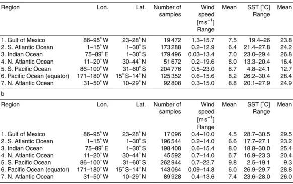
in radiometric experiments the sensitivity of H polarization to changes in wind, and thus to whitecap formation, was found to be larger than that of vertical V polarization (Anguelova and Webster, 2006; Anguelova et al., 2006). Figure 1 shows an example of the globalW distribution from WindSat for a randomly chosen day. The figure shows that the daily data do not provide global coverage. Due to the high variability in both
20
space and time, the daily W data cannot be interpolated to provide better coverage. Therefore, only the available data are used without filling the gaps for areas where data are lacking. This global data set was used to assess the wind speed dependence ofW
and devise a method to analyse regional variations (Sect. 3.1.1). The annual globalW
distributions show regions with either relatively low or relatively high numbers of valid
25
ACPD
15, 21219–21269, 2015Parameterization of oceanic whitecap fraction based on satellite observations
M. F. M. A. Albert et al.
Title Page
Abstract Introduction
Conclusions References
Tables Figures
◭ ◮
◭ ◮
Back Close
Full Screen / Esc
Printer-friendly Version
Interactive Discussion
Discussion
P
a
per
|
Discussion
P
a
per
|
Discussion
P
a
per
|
Discussion
P
a
per
|
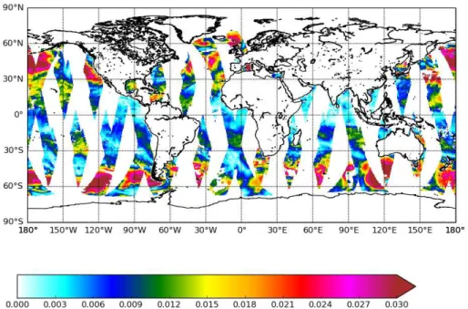
data points, and (ii) obtain a selection representative of both the Northern and South-ern Hemispheres (NH and SH). In this way, 7 regions of interest were selected (Fig. 2). The coordinates of the selected regions are listed in Table 1, together with the cor-responding number of samples, and range and mean values for wind speed and SST. Whereas regions 2–7 are all in the open ocean, region 1 was selected for its landlocked
5
position to identify the effect of short fetches. Although region 7 has, regarding its size, a relatively low number ofW samples compared to regions 1–6, it is included in the list to compensate for the otherwise limited representation of the Northern Atlantic Ocean. The results for this region could also show the degree to which the number of samples affects the informationW can give.
10
Following the results of the global data set assessment (Sect. 3.1.1), for each se-lected region, scatterplots of the square root of W against U10 were generated, and the best linear fits were determined. For the seasonal dependences, scatterplots were generated using all available daily data per month, ranging from 22 to 31 days of data.
2.3 Approach to derive whitecap fraction parameterization
15
The assessment of the satellite-based estimates of whitecap fraction (Sect. 3.1) in-forms our decision how to most effectively use these data to improve a whitecap-method based SSSF. The questions we considered were, (1) why develop aW(U10) parameterization instead of using satellite-basedW data directly; and (2) how to ac-count for the influence of secondary factors: explicitly, including them in the
parameter-20
ization, e.g.,W(U10, SST, atmospheric stability, etc.) or implicitly. These questions are addressed below.
A major benefit of using satellite-basedW data directly in an SSSF is that these data reflect the amount and persistence of whitecaps as they are formed by both primary and secondary forcing factors acting at a given location. This approach limits the
uncer-25
ACPD
15, 21219–21269, 2015Parameterization of oceanic whitecap fraction based on satellite observations
M. F. M. A. Albert et al.
Title Page
Abstract Introduction
Conclusions References
Tables Figures
◭ ◮
◭ ◮
Back Close
Full Screen / Esc
Printer-friendly Version
Interactive Discussion
Discussion
P
a
per
|
Discussion
P
a
per
|
Discussion
P
a
per
|
Discussion
P
a
per
|
does not provide daily global coverage; i.e., one would need data like that in Fig. 1 for at least two weeks (and more for good statistics) in order to have full coverage of the globe. Alternatively, a parameterization of whitecap fraction derived from satellite-basedW data can provide daily estimates of SSA emissions using readily available wind speed daily data. Importantly, such a parameterization will be globally applicable
5
because the whitecap fraction data cover the full range of meteorological conditions encountered over most of the world oceans. The availability of a large number of W
data would ensure low error in the derivations of theW(U10) expression.
Generally, to fully account for the variability of whitecap fraction, a parameteriza-tion of W would involve wind speed and the most important additional forcings
ex-10
plicitly (Anguelova and Webster, 2006; Salisbury et al., 2013), especially those readily available from either observations or meteorological forecasts, such asU10, SST, etc. However, a parameterization requiring the use of many variables is not conducive for application in global modeling. Therefore, a derivation of a W(U10) expression using data representative for a wide range of conditions, and thus implicitly accounting for
15
secondary forcing, is justifiable. We therefore set out to develop aW(U10) parameteri-zation which accounts for the secondary factors by a suitable functional choice of the
W(U10) relationship. To obtain a globally applicableW(U10) parameterization, we
aver-aged theW(U10) relationships derived for each of the considered regions and over all months (Sect. 2.2).
20
Ideally, when deriving a W(U10) parameterization, the data for W and U10 should
come from independent sources. The intrinsic correlation between W and U10 that might have arisen from the use of U10 from QuikSCAT in the estimates of W from
TB (Sect. 2.1), might affect the relationship between W and U10 developed here. To
evaluate the effect of this intrinsic correlation, U10QSCAT is replaced with U10 from the
25
ACPD
15, 21219–21269, 2015Parameterization of oceanic whitecap fraction based on satellite observations
M. F. M. A. Albert et al.
Title Page
Abstract Introduction
Conclusions References
Tables Figures
◭ ◮
◭ ◮
Back Close
Full Screen / Esc
Printer-friendly Version
Interactive Discussion
Discussion
P
a
per
|
Discussion
P
a
per
|
Discussion
P
a
per
|
Discussion
P
a
per
|
atmosphere-wave model (Goddijn-Murphy et al., 2011). Besides ECMWF wind data, for consistency we also extracted ECMWF SST values to use later in our analysis.
An additional advantage of quantifying the correlation betweenU10 from QuikSCAT andU10from ECMWF is the availability of the latter at 3 h intervals as compared to the
availability ofW–U10 pairs twice a day (Sect. 2.1). It is, therefore, preferred to derive
5
aW(U10) parameterization that is based on ECMWF wind speed data.
Quantifying the intrinsic correlation betweenW andU10from QuikSCAT comes down to quantifying how closely U10 from QuikSCAT and U10 from ECMWF correlate, for which these two quantities needed to be matched in time and space. To speed up cal-culation processes, and because this already provides a statistically significant amount
10
of data, only ascending satellite overpasses were used in the analysis. Wind speeds above 35 m s−1were discarded.
2.4 Estimation of sea spray aerosol emissions
The newly formulated W(U10) parameterization is applied to estimate the global an-nual coarse mode SSA emission with sizesr80 ranging from 1 to 10 µm. The particles
15
in the coarse mode consist, to a good approximation, solely of sea salt, whereas, in biologically active regions, the sub-micron size range additionally includes organic ma-terial, with an increasing contribution as particle size decreases (Facchini et al., 2008). Since the organic mass fraction in sub-micron sea spray aerosol particles is still highly uncertain (Albert et al., 2012) only the coarse mode SSA emission is estimated. As
20
suggested by Salisbury et al. (2014), the 37 GHzW data are more suitable to present the production of larger SSA particles than the 10 GHz data.
The emission of coarse mode SSA was calculated using a modeling tool (Albert et al., 2010), in which theW(U10) parameterization of MOM80, as integrated in Eq. (4), was replaced with the newly derived globally applicable W(U10) parameterization
25
ACPD
15, 21219–21269, 2015Parameterization of oceanic whitecap fraction based on satellite observations
M. F. M. A. Albert et al.
Title Page
Abstract Introduction
Conclusions References
Tables Figures
◭ ◮
◭ ◮
Back Close
Full Screen / Esc
Printer-friendly Version
Interactive Discussion
Discussion
P
a
per
|
Discussion
P
a
per
|
Discussion
P
a
per
|
Discussion
P
a
per
|
radius (e.g., Lewis and Schwartz, 2004; de Leeuw et al., 2011), and a density of dry sea salt of 2.165 kg m−3.
3 Results
3.1 Assessment of satellite-based whitecap fraction data
3.1.1 Wind speed dependence from global data set
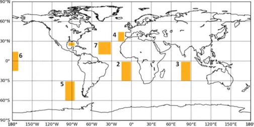
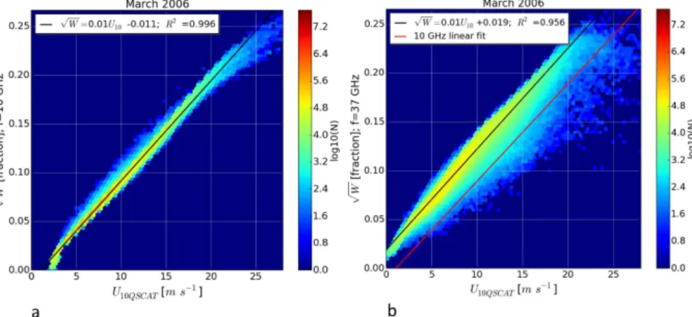
5
Figure 3 shows globalW data estimated from WindSat measurements for March 2006 as function ofU10QSCAT, at 10 GHz (Fig. 3a) and 37 GHz (Fig. 3b). For comparison, the MOM80 relationship (Eq. 2) is also plotted in each figure. The 10 GHz data show far less variability than those at 37 GHz. At 37 GHz, theW values at a certain wind speed vary over a much wider range, with the strongest variability for wind speeds of 10–
10
20 m s−1. This supports the suggestion that other variables, in addition toU10, influence
the whitecap fraction, such as SST or sea state. Salisbury et al. (2013) quantify this variability.
The 10 GHz scatterplot does not showW values for wind speeds lower than about 2 m s−1because at these low wind speeds no active breaking occurs, as mentioned in
15
the introduction. In contrast, at 37 GHz non-zero whitecap fraction values are retrieved at wind speedsU10<2 m s−1. Salisbury et al. (2013) suggested that the presence of
foam on the ocean surface at these low wind speeds could be due to residual long-lived foam. This residual foam might be stabilized by surfactants, which increases its lifetime (Garrett, 1967; Callaghan et al., 2013). Another explanation could be biological activity
20
(Medwin, 1977). However, there is not enough information currently to prove any of these conjectures.
ACPD
15, 21219–21269, 2015Parameterization of oceanic whitecap fraction based on satellite observations
M. F. M. A. Albert et al.
Title Page
Abstract Introduction
Conclusions References
Tables Figures
◭ ◮
◭ ◮
Back Close
Full Screen / Esc
Printer-friendly Version
Interactive Discussion
Discussion
P
a
per
|
Discussion
P
a
per
|
Discussion
P
a
per
|
Discussion
P
a
per
|
the resulting scatterplots:
p
W =0.01U10−0.011 10 GHz (5)
p
W =0.01U10+0.019 37 GHz (6)
with coefficients of correlationR2of 0.996 and 0.956, respectively. ThepW(U10) values at 10 GHz for wind speeds below∼3 m s−1were discarded in the analysis because, as 5
shown in Fig. 4, the linear relationship breaks up at about this wind speed. However, ei-ther discarding or taking into account these data points, does not significantly influence the position of the linear fit.
The quadratic trends ofW withU10 in Fig. 4 are in contrast to the known cubic and higher wind speed dependences such as in the MOM80 relationship. Using satellite
10
W data therefore results in a higher estimate of W at wind speeds lower than about 10 m s−1(based on Fig. 3a, obtained with 10 GHz data) and about 15 m s−1(based on Fig. 3b, with 37 GHz data), and a lower estimate for higher wind speeds. Wind speeds are generally lower than 10 or 15 m s−1 (cf. Fig. 3) and thus aW(U10) parameteriza-tion based on these data will most of the time lead to higherW estimates than those
15
obtained from using the MOM80 relationship.
3.1.2 Regional and seasonal variations
Figure 5 shows examples of the square root ofW againstU10QSCATfor different regions and seasons. Figure 5a–b shows scatter plots retrieved over the Gulf of Mexico (region 1) at both frequencies for January 2006. Statistics are presented at the top of the
20
figures and the fit lines are shown in red. Figure 5c–d shows the fit linespW(U10) for 10 and 37 GHz in region 5 for all months, while Fig. 5e–f demonstrates variations of the fit linespW(U10) for both frequencies over all regions for March 2006.
Figure 5 shows that the variations of the pW(U10) relationships at 10 GHz are smaller than those for 37 GHz, confirming the same observation reported by Salisbury
ACPD
15, 21219–21269, 2015Parameterization of oceanic whitecap fraction based on satellite observations
M. F. M. A. Albert et al.
Title Page
Abstract Introduction
Conclusions References
Tables Figures
◭ ◮
◭ ◮
Back Close
Full Screen / Esc
Printer-friendly Version
Interactive Discussion
Discussion
P
a
per
|
Discussion
P
a
per
|
Discussion
P
a
per
|
Discussion
P
a
per
|
et al. (2013) but obtained with a different analytical approach. Focusing on the results for 37 GHz, Fig. 5d and f shows that geographic differences from region to region for a fixed time period yield more variability in the pW(U10) relationship than seasonal variations at a fixed location, even for a location like region 5 where extreme seasonal changes could be observed. The standard deviation of the slopes in Fig. 5d is 3×10⁻⁴,
5
while that in Fig. 5f is 4×10⁻⁴. We surmise that obtaining whitecap fraction data at dif-ferent locations can ensure a wider range of meteorological and oceanographic condi-tions that influenceW than data at a fixed location for different seasons. This suggests that extreme yet sporadic seasonal values of the major forcing factor such asU10 at a given location contribute less to theW variations than varying environmental
condi-10
tions from different locations. Such observation has implications for collecting W data with the purpose of capturing and parameterizing the natural variability of whitecap for-mation and extent. For example, even if twice a day, satellite-based observations ofW
on a global scale are still an effective way to record influences of secondary factors. For in situ data collection, as could be expected, long-leg cruises would provide more
15
information on the effect of secondary factors, while long-term monitoring at a specific location will be more suitable to capture the wind speed effect alone.
Though noticeable, overall Fig. 5 shows small variations: the slopes of the resulting
p
W(U10) parameterizations for 12 months for all regions are found to be similar for all determined fits, about 0.01 with a standard deviation of 3×10⁻⁴. Sampling differences
20
between the regions (e.g., fewer samples in region 7 than in any other region) do not seem to cause significant differences between the resultingpW(U10) fits. Also, the re-sults from region 1 do not noticeably differ from the results from the other regions, or at least are within the spread of the different results. These outcomes do not provide sufficient information to draw conclusions on effects of short fetches. These small
vari-25
ACPD
15, 21219–21269, 2015Parameterization of oceanic whitecap fraction based on satellite observations
M. F. M. A. Albert et al.
Title Page
Abstract Introduction
Conclusions References
Tables Figures
◭ ◮
◭ ◮
Back Close
Full Screen / Esc
Printer-friendly Version
Interactive Discussion
Discussion
P
a
per
|
Discussion
P
a
per
|
Discussion
P
a
per
|
Discussion
P
a
per
|
extent. One possible explanation is that the additional influences have already been accounted for, at least partially, by using a quadratic power law. That is, the change from cubic to quadratic law is the change that the additional parameters impart on the
W(U10) relationship. Another suggestion might be that space and time variations of the
secondary factors exist, but because they affect W in opposite ways (e.g., Monahan
5
and O’Muircheartaigh, 1986), these influences cancel each other. Hence no further improvement can be expected by looking at effects of other factors on the variation in W explicitly, especially when the W(U10) dependence is derived from a database covering a wide range of conditions.
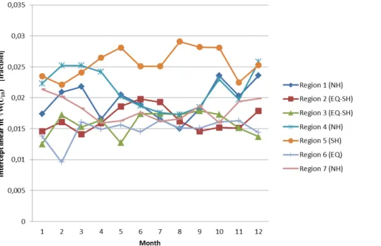
In contrast to the slope result, the intercept (i.e., the value forW at zero wind speed,
10
hereafter referred to as residual W) obtained with the 37 GHz W data shows strong variability (Fig. 6), with a mean value of 0.019, and a standard deviation of 0.004. These intercept variations at 37 GHz quantify the variations in absolute values of W
by region and season seen in Fig. 5d and f. The intercepts that were obtained with the 10 GHz data show much less variability with a mean value of−0.011 and a
stan-15
dard deviation of 9×10⁻⁴. Therefore, whereas 10 GHz data mainly provide the wind speed dependence ofW, the 37 GHz data set provides information useful to quantify the influence of secondary factors on W, such as SST, the presence and amount of surfactants, or the local relaxation time of foam, depending on conditions like viscosity (Salisbury et al., 2013).
20
These conditions are not only determined by the actual circumstances but also by the processes through which they developed, i.e. the history of environmental and meteorological quantities at a certain location, such as rising or waning winds, or the amount of foam that was already present as discussed in Sect. 3.1.1.
Although the intercept at 10 GHz has no physical meaning on its own, one can learn
25
Con-ACPD
15, 21219–21269, 2015Parameterization of oceanic whitecap fraction based on satellite observations
M. F. M. A. Albert et al.
Title Page
Abstract Introduction
Conclusions References
Tables Figures
◭ ◮
◭ ◮
Back Close
Full Screen / Esc
Printer-friendly Version
Interactive Discussion
Discussion
P
a
per
|
Discussion
P
a
per
|
Discussion
P
a
per
|
Discussion
P
a
per
|
sidering thatW values at 10 GHz are representative of predominantly active whitecaps, it is plausible to assume that new foam formation is less, if at all, affected by varying secondary environmental factors.
Because only the 37 GHz data provide information that represents different condi-tions on the globe, the remainder of the data analysis in this study will be based on
5
only these data.
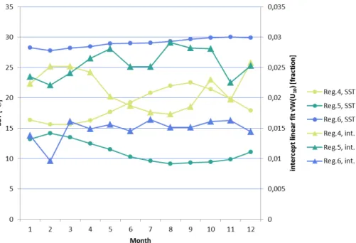
The results in Fig. 6 show a higher seasonal variability as the latitudinal distance from the Equator increases. This might point at some correlation with water temperature. Therefore, using the SST data for all months of 2006 at three regions extracted from the ECMWF database, the regionally averaged SST profiles are shown in Fig. 7 together
10
with the matching residualW. Figure 7 indicates that residualW and temperature are anti-correlated: with temperature increasing, the residual W roughly decreases. We discuss these results further in Sect. 4.
3.2 Parameterization of whitecap fraction
A parameterization ofW in terms ofU10was obtained by averaging thepW(U10)
rela-15
tionships for each region and for all months of 2006. The thus obtained relationship is similar to that derived from the global data set for only one month (Eq. 6):
p
W =0.01U10+0.020. (7)
The method used to quantify the intrinsic correlation between W and U10 from QuikSCAT is described in Sect. 2.3. Figure 8 shows all ECMWF wind speed data that
20
have been matched in time and space with the availableU10QSCATdata for March 2006. The majority of the data is clustered in the range of 5–10 m s−1. The correlation be-tween U10 from ECMWF (U10ECMWF) and U10 from QuikSCAT was determined as the best linear fit, forced through zero:
0.952·U10QSCAT=U10ECMWF→U10QSCAT=1.050·U10ECMWF, (8)
ACPD
15, 21219–21269, 2015Parameterization of oceanic whitecap fraction based on satellite observations
M. F. M. A. Albert et al.
Title Page
Abstract Introduction
Conclusions References
Tables Figures
◭ ◮
◭ ◮
Back Close
Full Screen / Esc
Printer-friendly Version
Interactive Discussion
Discussion
P
a
per
|
Discussion
P
a
per
|
Discussion
P
a
per
|
Discussion
P
a
per
|
with R2=0.844. On average, U10 from ECMWF is about 5 % lower than U10 from QuikSCAT.
We cast Eq. (7) in terms of U10ECMWF by combining it with Eq. (8). This allows for correction of the possible intrinsic correlation betweenW andU10, which is applied in the resultingW(U10) parameterization:
5
W =U10ECMWF2 +4U10ECMWF+4×10⁻⁴. (9)
This newly derivedW parameterization is compared to the MOM80 parameterization (Eq. 2) in Fig. 9, which shows the global annual averageW distributions for 2006 ob-tained with Eqs. (2) and (9) and wind speeds from ECMWF. The MOM80 relationship yields a wider W range with higher values in regions with the highest wind speeds,
10
as expected (see Sect. 3.1.1). In particular, this occurs over the southern oceans be-tween about 40 and 70◦S and in the North Atlantic between about 40 and 70◦N. The latitudinal variations from the Equator to the poles are more pronounced when using the MOM80 relationship as compared to Eq. (9). The new W(U10) parameterization provides a global spatial distribution with similar patterns, but the absolute values are
15
lower at high latitudes and higher at low latitudes.
3.3 Sea spray aerosol production
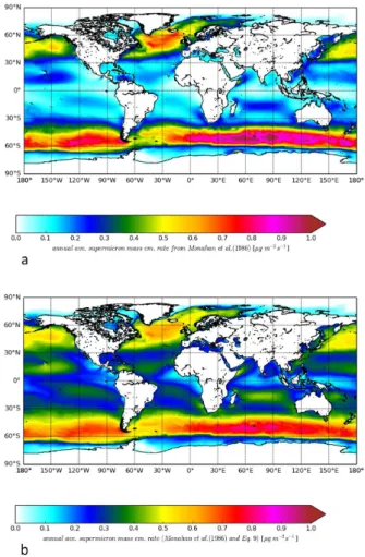
The newly derived parameterization was used to estimate how it affects the global annual average emission of coarse mode sea spray aerosol (Fig. 10). The spatial dis-tributions of the mass emission rates obtained with the new and the MOM80W(U10)
20
parameterizations mimic the patterns of theW distributions shown in Fig. 9. This is ex-pected because the M86 SSSF does not introduce variables that have a global pattern: the newW(U10) parameterization determines the spatial distribution whereas the M86 SSSF provides the factor to multiply with (3.575×10⁵).
Figure 11 shows the difference between the distributions of SSA mass emission rate.
25
ACPD
15, 21219–21269, 2015Parameterization of oceanic whitecap fraction based on satellite observations
M. F. M. A. Albert et al.
Title Page
Abstract Introduction
Conclusions References
Tables Figures
◭ ◮
◭ ◮
Back Close
Full Screen / Esc
Printer-friendly Version
Interactive Discussion
Discussion
P
a
per
|
Discussion
P
a
per
|
Discussion
P
a
per
|
Discussion
P
a
per
|
about 40 % larger than that calculated with MOM80 (Eq. 2), giving higher emission rates over a large part of the globe. Specifically, the total supermicron SSA mass emis-sion for 2006 is 2915 Tg (2.9×10¹²kg) when using the MOM80 W parameterization, and 4082 Tg (4.1×10¹²kg) when using Eq. (9).
4 Discussion
5
4.1 Assessment of satellite-based whitecap fraction data
The choice to use W data that were obtained at two different frequencies has led to more insight about the different stages ofW. Based on the findings obtained with 10 GHz data, it can be concluded that for stage A whitecaps, for open ocean, the only real forcing factor isU10, which mostly drives the absolute value ofW with little
vari-10
ations caused by other factors. Following from the analysis of the 37 GHz data, more information was obtained on stage B whitecaps, namely that the amount of stage B whitecaps also clearly depends on the wind speed, but effects of other factors con-tribute to larger variations of the absolute values.
When taking a closer look at the data cloud distributions of the scatterplots in Figs. 3
15
and 4, one can notice that the 10 GHz data show a relatively sharp cut-offon the bottom side of the data cloud whereas for the 37 GHz data one can see a sharp cut-offon the upper side. This might imply that at a certain wind speed there is a clear minimum of
W produced by active wave breaking, and a well set maximum of the total sum ofW. Apparently at a certain wind speed only up to a certain amount of foam can exist. One
20
could speculate on foam stability maxima constrained by wind speed but it should be considered that this might as well be an artifact of theW(TB) algorithm.
Considering our analyses of theW data sets, a lot seems to be explained byU10. Although not very significant compared to those that areU10-related, we do find some additional features as described below.
ACPD
15, 21219–21269, 2015Parameterization of oceanic whitecap fraction based on satellite observations
M. F. M. A. Albert et al.
Title Page
Abstract Introduction
Conclusions References
Tables Figures
◭ ◮
◭ ◮
Back Close
Full Screen / Esc
Printer-friendly Version
Interactive Discussion
Discussion
P
a
per
|
Discussion
P
a
per
|
Discussion
P
a
per
|
Discussion
P
a
per
|
First, Fig. 3 (the same applies for Fig. 5, showing data on regional scale) shows that at both 10 and 37 GHz a larger spread in W data is observed at higher wind speeds. Based on their different penetration depths, 10 GHz feels active (stage A) and only partially residual (stage B) whitecaps, while 37 GHz reacts on all, stage A and B whitecaps. However, we can expect that the situation would change for 10 GHz as wind
5
increases and with that the intensity and scale of the breaking waves. Because larger breakers form larger and deeper bubble clouds, thicker foam layers are expected on the surface not only for stage A but also for stage B whitecaps. Therefore 10 GHz will feel increasingly more stage B whitecaps as wind speed increases. With thicker residual foam at higher wind speeds, 10 GHz could be expected to become more variable due
10
to the larger influence of the secondary factors on the stage B whitecaps; this might explain the increased spread in the 10 GHz data.
Next, at the highest wind speeds, especially for W at 37 GHz, one can see some leveling off (saturation) of the satellite-based W, previously mentioned by Salisbury et al. (2013). A similar behavior was seen with the in situW data described in the work
15
by Callaghan et al. (2008). At higher wind speeds, the surface becomes quite com-plex with bubbles, foam, and spray, which might be a precursor of so called whiteout conditions as discussed by Holthuijsen et al. (2012). This leveling offin the whitecap fraction, similar to the leveling off of the drag coefficient (e.g., Zweers et al., 2010; Holthuijsen et al., 2012), is intriguing and deserves further analysis. However, before
20
claiming physical reasons for this feature, an extended scrutiny of theW(TB) algorithm is needed to rule out modeling causes.
Finally, it was found that residual W decreases with increasing temperature (Sect. 3.1; Fig. 7). A similar observation was reported by Bortkovskii and Novak (1993) as a result of an increase in the life-time of foam patches with decreasing SST which
25
ACPD
15, 21219–21269, 2015Parameterization of oceanic whitecap fraction based on satellite observations
M. F. M. A. Albert et al.
Title Page
Abstract Introduction
Conclusions References
Tables Figures
◭ ◮
◭ ◮
Back Close
Full Screen / Esc
Printer-friendly Version
Interactive Discussion
Discussion
P
a
per
|
Discussion
P
a
per
|
Discussion
P
a
per
|
Discussion
P
a
per
|
foam patches. Another factor that is confirmed to affect the life-time of residual W is the presence of surfactants at the ocean surface (Callaghan, 2013) which are more abundant at lower temperatures due to higher primary production (Falkowski et al., 1998), which increases bubble life-time and thus extends the life-time of residual foam (Salisbury et al., 2013). In a recent laboratory study by Callaghan et al. (2014), the
5
existence of an effect of water temperature on air entrainment and bubble plumes was confirmed. These authors concluded that the reported effects are far less significant compared to other factors affectingW, like e.g. wave field characteristics.
4.2 W(U10)-parameterization
4.2.1 Derivation of the newW(U10) parameterization
10
From the assessment of theW data with respect to variations on regional scales, the influence of secondary factors, in addition toU10, onW seems to be imbedded in the exponent of the wind speed dependence. It should therefore be reasonable to derive aW parameterization as a function ofU10 as it is simple enough for global modeling applications yet it incorporates the natural variability of whitecap fraction.
15
In the derivation of theW(U10) parameterization it was chosen to plot the square root ofW againstU10to weigh both axes evenly. Because the resulting scatterplots shaped up linearly, linear fits were applied to these scatterplots which, by simply squaring the average of the best linear fits, led to the final parameterization with a quadratic polyno-mial form. Summarizing the results of all regions by calculating the average did not lead
20
to a significantly different parameterization as was derived from the global data and it is therefore safe to use the global parameterization for global applications. However, when applyingW on a regional scale it should be preferred to use a regionally derived parameterization, since the differences between the regional parameterizations could be substantial as illustrated in Fig. 5f.
25
ACPD
15, 21219–21269, 2015Parameterization of oceanic whitecap fraction based on satellite observations
M. F. M. A. Albert et al.
Title Page
Abstract Introduction
Conclusions References
Tables Figures
◭ ◮
◭ ◮
Back Close
Full Screen / Esc
Printer-friendly Version
Interactive Discussion
Discussion
P
a
per
|
Discussion
P
a
per
|
Discussion
P
a
per
|
Discussion
P
a
per
|
favor of the quadratic relationship as found in this study (Eq. 9). It has been argued that
W should be proportional to the energy flux supplied by wind which is proportional to the cube of the friction velocityu∗ resulting in a cubic W(u∗) and above cubicW(U10) parameterizations (Wu, 1988). However, whitecaps are suppressed by swell (Sugihara et al., 2007; Salisbury et al., 2013) and thus not all of the energy that is supplied to
5
waves is dissipated through breaking waves and whitecap formation, but instead some energy is used to oppose swell conditions. This might explain the lower (quadratic) wind exponent derived in this paper, especially considering that on a global scale swell conditions are dominant over wind sea conditions (Salisbury et al., 2013). It should also be noted that many in situ data are obtained in regions dominated by sea wind
10
conditions (coastal regions or regions with a limited fetch), which should be kept in mind when comparing in situ studies with the work in this study.
To quantify the possible intrinsic correlation in the derivedW(U10) parameterization (Eq. 9), we have used ECMWF wind speeds instead of the QuikSCAT wind speeds (Sect. 2.3). We evaluate two aspects of theW,U10QSCAT, and U10ECMWF data used to
15
obtain theW(U10) relationship. One aspect is thatU10ECMWFvalues are about 5 % lower thanU10QSCAT(Fig. 8a and Eq. 8). This 5 % difference for theU10values up to 20 m s−1 leads to a difference in the whitecap fraction values of up to 8.5 %. TheU10differences between QuikSCAT and ECMWF can be explained to some extent with the effect of atmospheric stability because QuikSCAT provides equivalent neutral wind which
ac-20
counts for the stability effects on the wind profile (Kara et al., 2008), while the ECMWF model gives stability dependent wind speeds (Chelton and Freilich, 2005). Another as-pect is to evaluate the significance of the intrinsic correlation by looking at the change of the correlation coefficient of theW(U10) relationship when QSCAT winds are substi-tuted with the ECMWF winds. Physically, we expect a strong correlation between√W 25
andU10, and we see this clearly in Fig. 4 which shows a squared correlation coefficient
ofR2=0.956 for√W andU10QSCAT. However, the correlation coefficient might not be as high as in Fig. 4 ifU10 is from a more independent source. We show this in Fig. 8b which is similar to Fig. 4 but uses U10ECMWF. The
p
ACPD
15, 21219–21269, 2015Parameterization of oceanic whitecap fraction based on satellite observations
M. F. M. A. Albert et al.
Title Page
Abstract Introduction
Conclusions References
Tables Figures
◭ ◮
◭ ◮
Back Close
Full Screen / Esc
Printer-friendly Version
Interactive Discussion
Discussion
P
a
per
|
Discussion
P
a
per
|
Discussion
P
a
per
|
Discussion
P
a
per
|
seen in Fig. 8b, but the plot shows more scatter and the squared correlation coefficient isR2=0.826. The slopes in Figs. 4 and 8b differ by up to 10 %, a difference comparable to that of using neutral and non-neutral wind speeds. The finalW(U10) parameterization given with Eq. (9) was obtained by combining Eqs. (7) and (8). However, due to round-ing of the coefficients of the combined equation the final result is equal to the square of
5
Eq. (7), which means that the impact of Eq. (8) is lost in the process. We have checked the error that is introduced by the rounding and found that it leads to an underestimate ofW ranging from−6.5 % atU10=3 m s−1to∼ −10 % atU10=20 m s−1. Of course, we have to consider these differences in the light of other uncertainties in the parameteri-zation such as the goodness of the relationship betweenU10QSCAT andU10ECMWF and
10
the satellite-basedW data itself. We do not have a good estimate of neither of this at the moment. We therefore conclude that the effect of the intrinsic correlation onW, is presumed to lie within the error margins of the finalW(U10) parameterization given with Eq. (9).
For completeness, we have also investigated the effect of either rising or waning
15
winds on theW(U10) relationship. Although the value of W has been observed to be somewhat higher for waning than for rising winds, these differences are not statistically relevant. An effect of the wind history, therefore, is not included in the resultingW(U10) parameterization (Eq. 9).
The rise-wane (undeveloped-developed sea) effect as detected in this study is not
20
very pronounced compared to findings in studies that use in situ wind speed data (Stramska and Petelski, 2003; Callaghan et al., 2008; Goddijn-Murphy et al., 2011). Goddijn-Murphy et al. (2011) studied wind history- and wave development depen-dences on in situW data using either ECMWF wave model data, QuikSCAT satellite data, or in situ data forU10. These authors only detected significant effects with in situ
25
data forU10. The absence of a significant wind history effect in this study might
ACPD
15, 21219–21269, 2015Parameterization of oceanic whitecap fraction based on satellite observations
M. F. M. A. Albert et al.
Title Page
Abstract Introduction
Conclusions References
Tables Figures
◭ ◮
◭ ◮
Back Close
Full Screen / Esc
Printer-friendly Version
Interactive Discussion
Discussion
P
a
per
|
Discussion
P
a
per
|
Discussion
P
a
per
|
Discussion
P
a
per
|
whereas in situ data for wind speed are single point values averaged over a short time and hence representative for a relatively small area. The effect of the spatial averaging of the satellite data over a much larger area (i.e. the satellite footprint) might be that information on wind history is lost in the process.
4.2.2 Comparison with other functional relationships
5
In Fig. 12 the parameterization derived in this study (Eq. 9) is compared to W(U10) parameterizations obtained by MOM80, Callaghan et al. (2008), and Salisbury et al. (2013). The differences between the MOM80 parameterization and Eq. (9) are discussed in Sect. 3.2. Note that in most studies, as in this study, MOM80 is extrap-olated beyond the range of the data from which this parameterization was derived
10
(Monahan, 1971; Toba and Chaen, 1973). Therefore, at higher wind speeds theW val-ues that are obtained using the MOM80 parameterization are somewhat qval-uestionable. At the same time, the QuikSCAT instrument that provided theU10satellite data that are used in this study has a decreased sensitivity for wind speeds over 20 m s−1 (Quilfen et al., 2007). All results regarding higher wind speeds should therefore be handled with
15
caution.
The analyses in this study can be considered to complement the work of Salisbury et al. (2013, 2014) who also analysed satellite-based whitecap fraction data but with a different approach. These authors considered effects onW from a selection of quan-tities additional to U10 on a global scale, whereas in this study it was tried to visual-20
ize and identify effects of additional variables by comparing W data sets in different regions. Salisbury et al. (2013) report dependency ofW on secondary factors up to 25 %. On this basis, Salisbury et al. suggest to expand theW database with additional variables responsible for these effects to better quantifyW variability. By using a kind of top down approach, implicitly including all additional variables, this study comes to
25
ACPD
15, 21219–21269, 2015Parameterization of oceanic whitecap fraction based on satellite observations
M. F. M. A. Albert et al.
Title Page
Abstract Introduction
Conclusions References
Tables Figures
◭ ◮
◭ ◮
Back Close
Full Screen / Esc
Printer-friendly Version
Interactive Discussion
Discussion
P
a
per
|
Discussion
P
a
per
|
Discussion
P
a
per
|
Discussion
P
a
per
|
be sufficiently covered by the exponent of theW(U10) parameterization as discussed in
Sect 3.1.2, and in this sense it is not necessary to include additional variables.
There is little difference between theW(U10) parameterizations derived by Salisbury et al. (2013) (Eq. 1) and Eq. (9) derived here (Fig. 12). While on one hand this is to be expected because these parameterizations are based on similar data sets, it is
note-5
worthy that different analyses and parameterization approaches produced similar wind exponents, pointing to the robustness of the derivedW(U10) relationship. Differences that do occur can be explained by the somewhat different use of the same data. For ex-ample, in this study all availableW data are included in the analyses, while Salisbury et al. (2013) removed W data with a relative standard deviation (σW/W)>2, which
10
was about 10 % of allW estimates, mostly in regions with low wind speeds of around 3 m s−1, around the onset of foam formation.
Because differences with the alternative W(U10) parameterization derived by Callaghan et al. (2008) (Fig. 12) were previously discussed by Salisbury et al. (2013) and the differences between Eq. (9) and the Salisbury et al. (2013) parameterization
15
have turned out to be rather insignificant, we refer to this latter study for a detailed comparison.
However, a final remark can be made considering the method of obtainingW data, either from satellite, as in this study and the study from Salisbury et al. (2013), or in situ as in MOM80 and Callaghan et al. (2008). Callaghan et al. (2008) report a change
20
in slope inW1/3 as function ofU10 at wind speeds of around 10 m s−1. These authors suggest that the change in the dependence ofW onU10might indicate a different inter-action between wind and waves, due to the onset of spume droplet production between 9 and 11 m s−1. Another explanation was provided by Goddijn-Murphy et al. (2011) who suggest the appearance of underdeveloped waves at higher wind speeds, resulting in
25
ACPD
15, 21219–21269, 2015Parameterization of oceanic whitecap fraction based on satellite observations
M. F. M. A. Albert et al.
Title Page
Abstract Introduction
Conclusions References
Tables Figures
◭ ◮
◭ ◮
Back Close
Full Screen / Esc
Printer-friendly Version
Interactive Discussion
Discussion
P
a
per
|
Discussion
P
a
per
|
Discussion
P
a
per
|
Discussion
P
a
per
|
the direction in which the research vessel is moving. The emissivity of a breaking wave does have azimuthal dependence (Wentz, 1992). Considering the position of a vessel in higher winds facing waves that increase in height with increasingU10, it is plausible that W could be underestimated. The reported change in slope might then coincide with a certain wave height above which this underestimation exists.
5
4.3 Sea spray emission estimate
When modeling SSA emission, the impact of the modeling method used can be quite significant; e.g., Lewis and Schwartz (2004) report a spread in global emission esti-mates based on the M86 SSSF (Eq. 4), resulting from different studies, ranging from 3.3×10¹² to 11.7×10¹²kg yr−1, mainly caused by differences in model input data and
10
resolution differences (Grythe et al., 2014). Also, Table 2 in the work by de Leeuw et al. (2011) shows examples of the use of the same SSA production method lead-ing to significantly different results when applied in a different model. The two esti-mates made in this study, obtained with the M86 SSSF, including either the original MOM80 or the newly derived Eq. (9)W(U10) parameterization (Sect. 3.3), are
calcu-15
lated using the same modeling tool and input data. Similarly, Grythe et al. (2014) used the same model simulation to evaluate 21 SSSFs, including M86, against measure-ments. We thus can put our new estimate into perspective by comparing our results to those found in the Grythe et al. (2014, their Table 2) study. In the comparison, we scale the deviation between our and the Grythe et al. (2014) model using M86.
Specif-20
ically, using M86, Grythe et al. (2014) report two SSA emissions: an SSA estimate of 4.51×10¹²±0.44 kg yr−1 for the size range of 0.8 µm< r
80<8 µm, where the
esti-mated value is a 25 year average with an inter-annual variability range of±0.44, and an SSA emission of 5.20×10¹²±0.50 kg yr−1 for size range of 0.1 µm< r80<10 µm (referred to as M86E in Grythe et al., 2014). With regard to the size range, note that
25