www.ocean-sci.net/10/485/2014/ doi:10.5194/os-10-485-2014
© Author(s) 2014. CC Attribution 3.0 License.
The land-ice contribution to 21st-century dynamic sea level rise
T. Howard1, J. Ridley1, A. K. Pardaens1, R. T. W. L. Hurkmans2, A. J. Payne2, R. H. Giesen3, J. A. Lowe1, J. L. Bamber2, T. L. Edwards2, and J. Oerlemans3
1Met Office Hadley Centre, FitzRoy Road, Exeter, EX1 3PB, UK
2Bristol Glaciology Centre, School of Geographical Sciences, University of Bristol, University Road, Bristol, BS8 1SS, UK 3Institute for Marine and Atmospheric Research Utrecht, Utrecht University, P.O. Box 80005, 3508 TA Utrecht,
the Netherlands
Correspondence to:T. Howard ([email protected])
Received: 6 December 2013 – Published in Ocean Sci. Discuss.: 13 January 2014 Revised: 24 April 2014 – Accepted: 6 May 2014 – Published: 19 June 2014
Abstract. Climate change has the potential to influence global mean sea level through a number of processes includ-ing (but not limited to) thermal expansion of the oceans and enhanced land ice melt. In addition to their contribution to global mean sea level change, these two processes (among others) lead to local departures from the global mean sea level change, through a number of mechanisms including the effect on spatial variations in the change of water density and transport, usually termed dynamic sea level changes.
In this study, we focus on the component of dynamic sea level change that might be given by additional freshwater in-flow to the ocean under scenarios of 21st-century land-based ice melt. We present regional patterns of dynamic sea level change given by a global-coupled atmosphere–ocean climate model forced by spatially and temporally varying projected ice-melt fluxes from three sources: the Antarctic ice sheet, the Greenland Ice Sheet and small glaciers and ice caps. The largest ice melt flux we consider is equivalent to almost 0.7 m of global mean sea level rise over the 21st century. The tem-poral evolution of the dynamic sea level changes, in the pres-ence of considerable variations in the ice melt flux, is also analysed.
We find that the dynamic sea level change associated with the ice melt is small, with the largest changes occurring in the North Atlantic amounting to 3 cm above the global mean rise. Furthermore, the dynamic sea level change associated with the ice melt is similar regardless of whether the simu-lated ice fluxes are applied to a simulation with fixed CO2or under a business-as-usual greenhouse gas warming scenario of increasing CO2.
1 Introduction
Sea level rise (SLR) has the potential to lead to substantial impacts on society and ecosystems (Nicholls et al., 2011). Global mean SLR is comprised of thermal expansion, addi-tional meltwater from changes in land-based-ice mass bal-ance and other changes in terrestrial water storage (Church et al., 2011). Projected time-mean SLR for a particular loca-tion consists of a component from the global mean change, together with a component from changes in the spatial varia-tion of sea level relative to the global mean (e.g. Milne et al., 2009; Pardaens et al., 2011). This change in spatial variation is potentially influenced by the interplay of changes in ocean dynamics and spatial variations in density of the water col-umn. In addition, a change in the mass load of the land-based ice affects the sea level pattern through changes to the gravity field and through the vertical land movement response (giv-ing sea level “f(giv-ingerprints” of these changes in ice mass).
The largest uncertainty in projections of SLR to date is in the contribution from land-based ice melt, in particu-lar related to the enhanced ice sheet dynamics arising from ocean–ice sheet interactions (Pritchard et al., 2009). Key pro-cesses are increases in basal melt of ice shelves (Pritchard et al., 2012) and marine-terminating glaciers (Meier and Post, 1987) which lead to their thinning and consequent acceler-ated glacial discharge (Stanton et al., 2013).
models of the major outlet glaciers (Nick et al., 2013), or included in ice sheet models either as parameterisations of the flow-line models (Goelzer et al., 2013) or by enhanced basal sliding (Graversen et al., 2011) to capture the effect of increased glacial outflow.
Projected changes in the patterns of dynamic sea level (DSL), where this term is used here to denote the pattern of regional sea level change relative to the global mean, related to the ocean circulation, have been investigated in a number of studies. DSL is projected to change under the influence of greenhouse gas warming (e.g. Meehl et al., 2007; Lowe and Gregory, 2006), although there is considerable uncertainty in the pattern of SLR given by different models for projections under a common emission scenario (e.g. Gregory et al., 2005; Meehl et al., 2007; Pardaens et al., 2011). Some DSL stud-ies impose an increase in surface freshwater to the northern North Atlantic (“hosing”), and in some cases this additional water is confined around Greenland to represent additional ice sheet melt (Swingedouw et al., 2013). Many features of DSL change in the North Atlantic, both in projections un-der greenhouse gas warming and in hosing experiments, are related to a weakening of the meridional overturning circula-tion (MOC) (e.g. Levermann et al., 2005; Meehl et al., 2007; Lorbacher et al., 2010). The amount of weakening varies sub-stantially across models (e.g. Stouffer et al., 2006; Meehl et al., 2007). The effects of additional Greenland meltwater on the North Atlantic, together with ice mass change finger-prints, indicate that the DSL change associated with MOC slowdown is dependent on the ice melt geometry (Kopp et al., 2010).
In this study we develop projections of DSL change asso-ciated with new plausible scenarios of land-based ice melt. We assess two ice melt scenarios developed under the aus-pices of the European Union ice2sea project which include updated projections of the Glacier and Ice Cap (G&IC) contribution and Greenland and Antarctic ice sheet fresh-water contributions. The ice sheet components are derived from simplified simulations which include information about likely regions of glacial dynamic instability. The spatially and temporally varying glacial freshwater fluxes are applied in simulations with the HadCM3-coupled climate model (Gordon et al., 2000). The objective is to determine the de-tectability of DSL changes from the addition of these rel-atively small freshwater flux anomalies. We consider the role of this additional freshwater under both pre-industrial radiative forcing and under the Special Report on Emis-sions Scenarios (SRES) A1B greenhouse gas warming sce-nario (IPCC, 2000), which is usually regarded as a medium business-as-usual emissions scenario.
2 Scenarios of ice-melt freshwater flux
Two plausible scenarios are developed to describe changes in freshwater outflow to the ocean from land-based ice mass
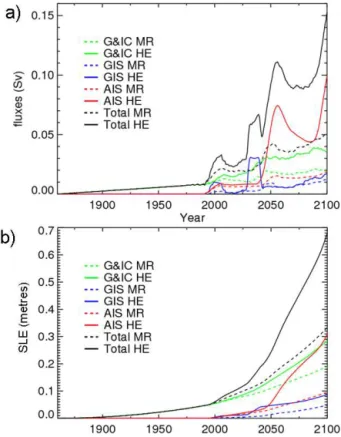
Figure 1. Global-mean freshwater fluxes from land-based ice masses. Panel(a): in Sv (Sverdrups),(b): cumulative, in sea level equivalent (SLE). Note that part of the ice which is melted is dis-placing water prior to melt, so while it contributes to the freshwater into the ocean, it would not contribute to sea level rise. The actual contribution to sea level rise from the fluxes may therefore be less than the SLE of Fig. 1b).
changes. For glaciers and ice caps and for Greenland calv-ing, these are derived from upscaling process-based mod-elling of the respective ice masses. The Greenland surface runoff changes are obtained by downscaling a global climate model projection. The Antarctic ice sheet component is de-rived from simplified simulations which include information about likely regions of dynamical instability. The generation of each component of freshwater outflow in the scenarios in-volved the use of climate forcing from an SRES A1B projec-tion by the ECHAM5-coupled climate model (Roeckner et al., 2006), so giving a measure of self-consistency between the components. The two scenarios are a representative mid-range (MR) and an illustrative high-end (HE) scenario. The contributions from each freshwater component are described in the following subsections; further detail on the construc-tion of these scenarios can be found in Spada et al. (2013).
Figure 2.Ocean grid points involved in freshwater forcing by ter-cile of integrated freshwater flux (coloured), other ocean grid points (grey) and land grid points (white).
particular component was assumed to be in steady state). The freshwater flux anomalies are applied to the nearest of 28 HadCM3 coastal ocean sectors (16 for G&IC, 5 for Green-land and 7 for Antarctica) and distributed equally to all grid cells along that sector (see Fig. 2).
While these scenarios have been developed using climate projections from a particular model and under the A1B sce-nario, the basal sliding perturbations applied to the ice mod-els to obtain the HE scenario are likely to give a change in meltwater flux that dominates over uncertainties over climate forcing (Bindschadler et al., 2013). The timing of shorter timescale variability in the scenarios, however, should only be thought of as illustrative of the sort of ice mass behaviour that might be obtained.
2.1 Glaciers and ice caps meltwater component
The glaciers and ice caps (G&IC) component of ice mass change was derived from a regionalised glacier mass bal-ance model that uses projected temperature and precipita-tion anomalies for 19 glacierised sectors (Giesen and Oer-lemans, 2013). In this model, sensitivities of the regional G&IC responses were calibrated using automatic weather station data, of temperature and precipitation, for 80 bench-mark glaciers (Giesen and Oerlemans, 2012). This calibrated version of the projected volume changes (1980–2100) was used for the MR scenario and the HE scenario was ob-tained by simply perturbing the melt parameters to their up-per plausible limit. Only the equivalent positive fluxes of net-meltwater were transferred to the ocean with these assumed, as an approximation, to be solely due to an increase in melt-runoff rather than from any reduction in accumulation. An approximate G&IC steady state (with zero flux anomalies) was assumed for 1860, with the calculated fluxes interpo-lated back to this point. Fluxes from the ice sheet peripheral
G&IC, not directly attached to the ice sheet, were assigned to the G&IC water flux.
The total sea level equivalent (SLE) of the G&IC fresh-water fluxes, for the 2090–2099 period relative to the 1980– 1999 period is 0.13 m and 0.22 m for the MR and HE scenar-ios respectively. These estimates are in good agreement with other projections. Projections for the G&IC component of sea level rise from the 5t hCoupled Model Intercomparison Project (CMIP5), relative to the 1986–2005 mean at 2100, are: 0.17 m (RCP4.5) to 0.22 m (RCP8.5) (Marzeion et al., 2012). A similarly derived independent estimate which takes into account dynamic processes, like the thinning and retreat of marine-terminating glaciers, provides an estimated contri-bution from G&IC of 0.10 to 0.25 m to sea level rise by 2100 (Meier et al., 2007).
2.2 Greenland Ice Sheet meltwater component
Projected changes in freshwater flux from the Greenland Ice Sheet surface mass balance (such fluxes are hereafter re-ferred to as runoff) and from iceberg calving are considered. The projected runoff anomalies are obtained from a simu-lation by the regional MAR model (Fettweis et al., 2007), which provides a downscaling from the ERA-Interim reanal-ysis (1989–2000) and an ECHAM5 projection (2001–2100) following the A1B emissions scenario. We do not perturb surface runoff for the HE scenario as it is not directly affected by the primary ice dynamics uncertainties. A model inter-comparison (Bindschadler et al., 2013) shows that the steastate ratio between surface mass balance anomaly and ice dy-namical discharge flux varies between 0.25 and 0.9. A steady state was assumed at 1992, prior to the observed increase in both the runoff and calving fields. The runoff anomalies applied to the HadCM3 ocean are relative to a 1989–1995 baseline, centred on this “steady-state” year.
The Greenland calving contribution to the freshwater flux into the ocean is a function of the ice sheet dynamics and is calculated from upscaling flow-line simulations for three outlet glaciers, Jakobshavn Isbrae, Petermann and Helheim (Nick et al., 2013), to the rest of Greenland. The glacier sim-ulations of Nick et al. (2013) were calibrated against present-day observations for the MR scenario. The ice sheet sliding at the bedrock was increased by its two-sigma error estimate to generate new flow-line simulations for the HE scenario. The upscaling to three coastal sectors, representative of the three glaciers, was based on the approach of Price et al. (2011).
temperature in the particular forcing projection, which is in line with evidence of an ocean-forced synchronised glacier acceleration in SE Greenland (Christoffersen et al., 2011) and SW Greenland (Holland et al., 2008) in the early 2000s. The simplified simulations used here may, however, overem-phasise the degree of synchronicity.
The calving component, referenced to 1992, gives 5 mm (MR) and 56 mm (HE) sea level rise values by 2100. For comparison, recent modelling of the whole ice sheet (Goe-zler et al., 2013) identifies a range of 4 to 12 mm, while Gra-versen et al. (2011) and Furst et al. (2013) identify higher-end values of 16 and 45 mm respectively. However, these models do not explicitly address the issue of the fast flow-ing tidewater glaciers simulated by Nick et al. (2013) where the fast dynamical component is estimated to be (referenced to the 1986–2005 mean) 85 mm for representative concen-tration pathways (RCP)8.5 and 63 mm for RCP4.5 by 2100. Thus, as a whole, there is considerable uncertainty for the future dynamical changes to the ice sheet, but our own esti-mates are arguably at the low end for the MR scenario. For Greenland, the overall SLE (calving and runoff) values for our MR and HE scenarios are 0.04 m and 0.08 m by 2100, while the fifth Assessment Report of the Intergovernmen-tal Panel on Climate Change (AR5) medians are 0.08 m for RCP4.5 to 0.12 m for RCP8.5 (Church et al., 2013).
2.3 Antarctic ice sheet component of freshwater
For the Antarctic ice sheet, the projected freshwater fluxes into the ocean are assumed to come from iceberg calving and the marine melt of ice shelves alone (surface runoff being negligible). These fluxes are derived from the simulations of Ritz et al. (2014). The ice sheet model is not fully cou-pled with an ocean component, and consequently grounding line retreat scenarios are imposed on the modelled ice sheet, taking account of regions of likely dynamic instability. The simulations include the ice shelf basal melt, leading to rapid ice dynamics, and grounding line retreat, which leads to ma-rine ice sheet instability (Binschadler, 2006). The resulting 1000-model ensemble has individual members weighted ac-cording to their success in simulating present-day sea level contribution. The HE estimate is that of a single member that lies close to the ensemble 99.9 % probability threshold for ice mass loss, while the MR estimate is a single member closest to the maximum likelihood at 2100. The associated component of SLR, between 2006 and 2100, is 311 mm for HE and 99 mm for MR. For comparison, the SLE (from the rapid ice dynamics alone) for AR5 is 70 mm in both RCP 4.5 and RCP8.5.
Time smoothing (11 years) of the Antarctic fluxes is jus-tified because the icebergs take several years to melt, which would act as a natural smoothing function. The large tran-sient pulses of freshwater which remain arise from marine ice sheet instability, with the rapid retreat of the grounding line resulting in large losses of ice. The first peak is
associ-ated with a partial collapse of the West Antarctic Ice Sheet in the region of Pine Island Bay, as predicted (Cornford et al., 2013). The final peak occurs with another partial collapse of the West Antarctic Ice Sheet in the region of the Filchner Ice Shelf as depicted in some simulations (Hellmer et al., 2012). In accordance with present-day observations (Pritchard et al., 2012), most of the melt occurs in the Amundsen Sea (west of the Antarctic Peninsula). A steady state is assumed in 1992, as for Greenland, as this was when the first evi-dence of instabilities in the ice sheet was suggested (Doake and Vaughan, 1991; Jacobs et al., 1992), with the freshwater fluxes interpolated back to zero anomalies at this time.
2.4 Scenario global total freshwater fluxes
The total SLE values for the MR and HE scenarios for 2090– 2099 (referenced to 1860–1870) are 0.26 and 0.57 m respec-tively, while from AR5 the median SLR values given from all land-based ice masses are 0.27 m (RCP4.5) and 0.35 m (RCP8.5). As we noted in Sect. 2.3, these estimates include the ice sheet rapid dynamics, but not the marine ice sheet instability (which dominates the SLE at 2100 for the HE sce-nario) nor the accumulation on Antarctica.
3 HadCM3 model formulation
The simulations used in this study to provide projections of sea level patterns under the ice melt scenarios are ini-tialised from a long HadCM3 “control” simulation1, which has fixed pre-industrial radiative forcing (appropriate to 1861). HadCM3 (Gordon et al., 2000; Pope et al., 2000) is a coupled atmosphere–ocean general circulation model (AOGCM). The atmosphere model has a resolution of 3.75 degrees longitude by 2.5 degrees latitude with 19 vertical lev-els. The ocean model has a resolution of 1.25 degrees longi-tude by 1.25 degrees latilongi-tude with 20 vertical levels. The sea ice model uses a simple thermodynamic scheme including leads and snow cover, with ice advected by the surface ocean current. The ocean model has a rigid lid surface boundary condition with surface freshwater fluxes applied as a virtual salt flux; a reference salinity of 35 psu is used to avoid a global average salinity drift. Changes in sea surface height are calculated in a post-processing step, using the method described by Lowe and Gregory (2006).
The standard HadCM3 control simulation ran for more than two thousand years after initialisation, with the ocean spun-up from rest and with initial potential temperature and salinity data from the World Ocean Atlas (Levitus et al., 1The standard HadCM3 control simulation was continued for
1994; Levitus and Boyer, 1994). HadCM3 simulations have been extensively analysed: for example, the time-mean ocean quantities in the control simulation (e.g. Gordon et al., 2000; Pardaens et al., 2003) and aspects of variability (e.g. Vellinga and Wu, 2004). The scenarios of additional ice-melt flux for this study were applied to both the HadCM3 control simu-lations and also to simusimu-lations under the SRES A1B green-house gas warming scenario.
The SRES A1B projection was initialised from a histor-ical period simulation which was, in turn, initialised from the control simulation. Radiative forcing changes appropriate to the period of time-varying greenhouse gas concentration were applied following the methodology of Forster and Tay-lor (2006), which offers a simplified equivalent A1B forcing in terms of CO2alone: these forcings were diagnosed from the original IPCC Third Assessment Report HadCM3 simu-lations. The 21st-century changes in sea surface temperature, salinity and DSL in the northern Atlantic were broadly sim-ilar to the climate changes seen under the original HadCM3 A1B simulation.
There is no explicit representation of iceberg calving in HadCM3, so a time-and-scenario invariant prescribed wa-ter flux is returned to the ocean (Gordon et al., 2000). This fixed magnitude water flux is calibrated to approximately balance, on a multi-century timescale, the net snowfall ac-cumulation on the ice sheets under pre-industrial conditions; it is geographically distributed within regions where bergs are found (Gladstone et al., 2001). The prescribed ice-berg freshwater flux amounts to 0.03 Sv (Sverdrups) from Greenland, larger than 0.2 Sv estimated from reconstructions (Hanna et al., 2011) and 0.09 Sv for Antarctica. We leave this term unchanged, as it forms part of the baseline “equi-librium” state of ice-melt-related freshwater flux. In addi-tion, the HadCM3 model simulates runoff from the ice sheets which increases with greenhouse gas forcing, as the sur-face mass balance changes. The scenarios of ice melt we are using, however, incorporate their own changes in ice sheet runoff, as derived from the MAR regional model. To avoid double-accounting for projected changes in surface runoff, the model-generated runoff is switched off. The baseline cli-matological seasonal cycle of runoff, to which the projected anomalies are then added, is derived from a section of the HadCM3 pre-industrial control simulation.
Glaciers and small ice caps are not explicitly represented in the coarse resolution HadCM3 model, so the scenario anomalies of freshwater flux from such ice are simply added to coastal outflow points.
To compensate for model climate drift, locally or in glob-ally integrated quantities, a low-pass temporal filter is applied to 600 years of the parallel control simulation. This filtered signal is taken to be the model drift and we take this into ac-count for our analyses (Sect. 4) of changes in DSL and other quantities. However, our results are not sensitive to omitting this drift compensation, indicating that the amount of drift over this period is small.
4 DSL changes induced by scenarios of land-based ice melt under pre-industrial baseline conditions
In this section we present the change in DSL patterns (i.e. excluding global mean sea level changes) which are associ-ated with the ice-melt scenarios. To reduce the influence of unforced variability, the mean of a three-member ensemble with pre-industrial radiative forcing is analysed. Two mem-bers of the ensemble differ in their initial conditions, these being taken from points on the control simulation separated by 250 years. The third member shares initial conditions with the first, but the model’s own internal simulation of the pre-industrial baseline runoff from the ice sheets is treated dif-ferently (see Sect. 2.2). We assert that this subtle change in the model makes a comparable difference to the use of different initial conditions by the time the strong ice-melt forcing is applied: about a hundred years after initialisation. Evidence to support this assertion comprises the difference in Atlantic meridional overturning circulation (AMOC) be-haviour (Sect. 6) and the difference in the evolution of a sim-ple scalar measure of the DSL change (Sect. 4.2).
The general approach in assessing the simulations is to identify the patterns associated with the mean DSL change for the mean of the last 100 years of the freshwater outflow scenarios, when the ice melt is strongest (Fig. 1) with respect to the mean of the first 100 years. A more detailed analysis is carried out for a case study of the northern Atlantic: the time evolution of the DSL pattern in this region is analysed and a regression analysis of DSL and of the corresponding tem-perature and salinity changes against the meltwater forcing is also used to facilitate a mechanistic analysis of the change.
4.1 Time mean DSL changes
Significant regions of DSL change, averaged over the final 100 years of the HE scenario, are identified using two crite-ria: (1) the sign of the forced anomalies at each model grid point is the same in all three simulations and (2) the abso-lute value of the ensemble-mean change (at each model grid point) is greater than two standard deviations (2σ) of the dis-tribution of 100-year-mean unforced changes from sequen-tial periods of the control simulation at each grid point. Note that this is a stricter criterion for the ensemble mean than for the individual forced simulations. No significant pattern of DSL change is found when these same criteria are applied to a mean of the final 100 years of the concurrent three sections of control simulation. This methodology to identify signifi-cant changes is based on, but not identical to, that proposed by Livezey and Chen (1983).
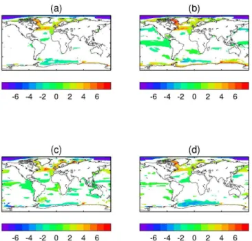
Figure 3.DSL anomalies (cm) under the HE ice-melt scenario and for pre-industrial baseline conditions, averaged over years 2000– 2099. Anomalies are relative to the concurrent period of the low-pass filtered control as described in the main text. Panel(a): mean of the three forced simulations. Panels (b), (c)and (d)show the three simulations separately. Coloured regions show where anoma-lies are greater than 2σ of the distribution from the control simula-tion. A stricter criterion is applied to(a): see main text. Note that the patterns shown are anomalies in two senses: first, because they are relative to the concurrent period of the low-pass filtered control and second, because they exclude any change in the global mean sea level.
these regional deviations on local SLR under the HE scenario is relatively small, the DSL deviation is about 3 cm in the North Atlantic, whilst the global mean SLR from ice melt is 57 cm. The size of this contribution is put into the context of some of the other contributions to regional sea level change by Howard et al. (2014).
The fairly small magnitude of the DSL response to our ice melt scenarios is not inconsistent with that found in the hosing experiments of other studies, once the differ-ent levels of freshwater flux are accounted for. For ex-ample Swingedouw et al. (2013) show DSL impacts of a 0.1 Sv hosing around Greenland averaged over the fourth decade of hosing for four different models (their Fig. 16). By the middle of that decade, the ocean receives 3.5 Sv-years of accumulated anomalous freshwater forcing from Green-land. By the middle of our averaging period of 2000–2099, our ocean receives only around 0.6 Sv-years from Green-land (and about 3 Sv-years in total, globally). Taking the minimum-to-maximum sea level height difference in the North Atlantic as a simple measure of the strength of the ocean DSL response, the Swingedouw et al. (2013) model intercomparison shows a response of around 40 cm
(Insti-tut Pierre-Simon Laplace: IPSL-CM5); 10 cm (Max Planck Institute-earth system model: MPI-ESM); 25 cm (European Centre for Medium-Range Weather Forecasts Earth System Model: EC-Earth) and 30 cm (GEOMAR Helmholtz Centre for Ocean Research Global Ocean Model: ORCA05). Our corresponding value is around 8 cm, which does not seem out of place given the weaker forcing in our simulation. Our spatial pattern of DSL response in the North Atlantic lies within the envelope of patterns presented by Swinge-douw et al. (2013), with a maximum sea level rise around 45◦N, 30◦W and a marked spatial similarity to the pattern of ORCA05 (though with different magnitude, as discussed above).
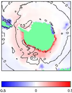
Our HE ice scenario simulations (Fig. 3b, c, d) show pat-terns of response, albeit weak, in the tropical Pacific, a re-gion where the unforced variability, on 100 year timescales, is low. In the Southern Ocean, the freshwater input is substan-tial (around 4.5 Sv-years by the end of the simulation). Of this, 95 % is to the Bellingshausen and Amundsen seas, west of the Antarctic Peninsula, leading to a surface freshening (0.9 psu) and stratification of the waters near the coast. The stratification leads to a build-up of advected heat in the in-termediate waters down to 1000 m (Fig. 4) leading to a small thermosteric sea level rise. This behaviour is in good agree-ment in the processes described by Stouffer et al. (2007), with increased incidences of deep convection resulting from the warmer deep waters similar to that found by Keeling and Visbeck (2011). With very little glacial melt in the Weddell Sea region, the stratification there is relatively weak (0.2 psu) until the last decade of the simulation. There is no discern-able change in the Antarctic Circumpolar Current (ACC) vol-ume or freshwater transport though the Drake Passage (not shown). However, the barotropic stream function of the Wed-dell and Ross sea gyres increases (Fig. 4) which is consistent with a drop in the sea level within each gyre (Fig. 3) to main-tain geostrophic balance. A similar effect in the Ross Sea is offset by the increase in oceanic heat content.
The ocean stratification around Antarctica leads to a fairly uniform and statistically significant 10 % increase in the sea ice cover over the last 50 years of the simulation. How-ever, despite a considerable freshwater input to the South-ern Ocean late in the time series, we do not see a clear link between Southern Ocean and North Atlantic MOC as sug-gested by Swingedouw et al. (2009). It is possible that the lag in affecting the MOC in HadCM3 is longer than the 50 years, and consequently the freshwater input to the Southern Ocean would influence the response of the MOC after the end of the simulation.
The high Arctic also shows a significant fall in DSL, prin-cipally in the Beaufort Sea. This appears to be linked to an inflow of saline warm water from the Atlantic. The slight warming of near-freezing waters results in an increase in den-sity and subsequent fall in DSL.
Figure 4.The changes around Antarctica of mean ocean temper-ature (colour) and barotropic stream function (contours in Sv). Anomalies are the ice-melt ensemble mean for the last 40 years ref-erence to the equivalent years of their unforced control simulations.
al. (2013), in which the Atlantic pattern of DSL rise was linked to the pathway of freshwater leakage from the subpo-lar to subtropical gyres. Differences in model asymmetries of the subpolar gyre shape and barotropic stream function, as well as responses of the MOC, contribute to the uncertainty. Large uncertainties were found for the DSL response in the Arctic and were attributed to the transport pathways of At-lantic water, with various effects on the sea ice edge in the Barents Sea. In their intercomparison, HadCM3 had a rela-tively large amount of freshwater leakage from the sub-polar gyre into the Canary current and a relatively small weaken-ing of the MOC (HadCM3 was not included in their DSL intercomparison). Our result is similar in magnitude of DSL rise to a transient simulation with the MIT General Circu-lation Model (MIT GCM) (Stammer, 2008). That simula-tion resulted in a more widespread distribusimula-tion of water from Greenland melt, with quite a different pattern in the North At-lantic, but a similarly confined impact on the global oceans from Antarctic melt.
Stammer et al. (2011) using the University of California, Los Angeles model investigated the response of both a cou-pled ocean-atmosphere model and an ocean-only model to enhanced Greenland freshwater forcing of 0.0275 Sv sus-tained for 50 years. This forcing is stronger than the Green-land component of our forcing, but even taking account of this (and even ignoring the other components of our forcing) Stammer et al. (2011) report a noticeably stronger response in the DSL pattern than the pattern which we see, particularly in their coupled simulation. Further, despite some similari-ties in the equatorial regions, the Southern Ocean and most
noticeably the Labrador Sea, their pattern of response is gen-erally quite different to ours.
In the following two subsections, we focus on the pattern of DSL change in the northern Atlantic, to further examine the mechanisms of change. The ensemble-mean patterns are similar for the MR and HE ice melt scenarios (unmasked global correlation coefficient of 0.83, unmasked North At-lantic correlation coefficient of 0.93 and see also Fig. 5), but differ in magnitude, with smaller deviations under the MR scenario. We now consider how the scaling in the response compares with the scaling in the forcing by comparing a crude scalar measure of each.
An area-weighted simple linear regression of the un-masked global MR DSL pattern against the unun-masked global HE DSL pattern has a gradient of 0.67 (or 0.63 using the North Atlantic only). This is our crude measure of the MR : HE scaling in the response. A crude measure of the scaling in the forcing affecting the North Atlantic is the MR : HE ratio of the ice-melt flux integrated over the North-ern Hemisphere and over the period of the simulation. This ratio is 0.63.
Given the similarity of these simple measures of the scal-ing in the response and forcscal-ing, we scaled the HE DSL pat-tern by a factor of 0.63 to make a predictor of the MR DSL pattern. The difference between the MR pattern and the pre-dictor is shown in Fig. 5c.
The similarity of the patterns in MR and HE scenarios sug-gests that the pattern might be fairly time-invariant over a range of increasing Greenland ice melt; however the low am-plitude of the DSL change makes this difficult to robustly identify, as the signal only becomes statistically significant in long-term means. Given the similarity of the identified DSL pattern changes under HE and MR ice melt scenarios (c.f. Fig. 5a, b, c), we assess only the HE scenario in the follow-ing subsections.
4.2 North Atlantic case study: time evolution of DSL response to HE ice melt scenario
In order to study the time evolution of the northern At-lantic DSL response to the ice melt scenarios (Sect. 4.1), we project the simulated year-by-year DSL anomaly (denoted
si(t ), wheret is year andiis grid point) onto the previously
identified (Sect. 4.1) mean pattern of DSL change for this re-gion (pi), as depicted in Fig. 5a. The projectionπ(t ), which
can be thought of as the component ofpi present insi(t ), is
the scalar product ofsi(t )and normalisedpi:
π(t )=cov√(s(t ), p)
var(p) =
Ps
i(t )piwi
q Pp2
iwi
Pw
i
(1)
The covariance and variance calculations are area-weighted bywi, the area of grid-pointi. This is essentially the
Figure 5. DSL anomalies (cm) in the northern Atlantic.
(a): ensemble-mean significant anomalies for HE ice-melt scenario, as Fig. 3a, but showing detail of the northern Atlantic.(b): the same for MR ice-melt scenario.(c)shows, using the same colour scale, the error in using the scaled HE anomalies as a predictor of the MR anomalies (see main text; negative errors indicate under prediction).
further normalise by√var(p)to give a dimensionless index. Of the three quantities si(t ),pi andwi, onlysi(t )changes
year-to-year. The projectionπ(t )gives a simple scalar mea-sure of the time-evolution of the DSL anomaly.
The relationship of π(t )with the time-varying ice-melt-scenario-flux, is seen by comparing π(t )with the ice-melt flux integrated over the Northern Hemisphere (Fig. 6). Both the gradual increase and, arguably, some of the shorter-term
Figure 6.Relationship between the ice-melt flux integrated over the Northern Hemisphere (thick grey line) for the HE scenario, and the year-by-year projectionπ(t )(not smoothed) onto the North At-lantic DSL pattern which was identified as being associated with the ice-melt (Fig. 5a). Panel(a): for the ensemble mean DSL anomaly (thin black line)(b)for DSL anomalies in each simulation (coloured lines).
variability of the ice flux are reflected in the evolvingπ(t )
(Fig. 6a). There is no clear and notable time lag betweenπ(t )
and the variations in ice flux. Both the inter-annual to decadal variability and ensemble-spread ofπ(t )are significant com-pared to the century-scale change inπ(t ), consistent with our argument that the dynamic sea level change associated with the ice melt is small. The two forced ensemble members with common initial conditions (see Sect. 4) are shown by the red and blue lines in Fig. 6b.
As discussed in Sect. 4.1, the DSL anomalies in the forced simulations are statistically significant even though they are small. Evidence for the statistical significance of the time-evolving DSL anomaly as measured byπ(t )is presented in Fig. 7. In brief, this figure shows that π(t )for the forced simulations (broken black lines) evolves to be well outside the noise ofπ(t )for the control simulations (red and blue lines).
Figure 7.Projectionπ(t )of each year’s DSL anomaly field onto a pattern of change. Panel(a): three individual HE forced simulations (broken black lines) projected onto the HE forced pattern of Fig. 5a and the three corresponding sections of control (red lines), projected onto the HE forced pattern of Fig. 5a. Panel(b): Year-by-year aver-age of the three HE forced simulations shown in(a)(broken black line) and year-by-year average of the three parallel sections of con-trol shown in(a)(red line). Also shown are eight blue lines. Each of these shows a year-by-year average of a set of three sections of control with start years chosen at random, again projected onto the HE forced pattern of Fig. 5a. Panel(c): broken black lines exactly as in(a)and, for comparison, the three corresponding sections of control (red lines), this time projected onto the mean anomaly of the final hundred years of these three sections of control simulation (i.e. projected onto their “own” pattern). Panel(d): broken black lines exactly as in (b)and, for comparison, red line shows year-by-year average of the three sections of control shown in(c). Also shown are eight blue lines. Each of these shows a year-by-year av-erage of a set of three sections of control with start years chosen at random, again projected onto their “own” pattern. The point is that the forced signal (broken black line) evolves to be well outside the unforced noise (red and blue lines).
projected onto a pattern derived from the control simula-tions, in panels c and d; (red and blue lines). The message is clearest when we consider means over three simulations: panel b shows that the forced-on-forced projection evolves outside the noise of thecontrol-on-forced projection. Panel d shows that theforced-on-forcedprojection evolves outside the noise of thecontrol-on-controlprojection. In panels a and c the unforced variability (noise) is sampled by the three-member parallel control ensemble only. Using the whole of our long control simulation (1715 years), we are able to study a larger sample of the noise by taking sets of three 240-year chunks (with initial times chosen randomly from within the long control simulation) and treating them in the same man-ner as the three-member parallel control ensemble. We cre-ated eight such sets: the results are the eight blue lines in each of panels b and d in Fig. 7.
Figure 8.Regression of ensemble-mean DSL against ice-melt flux integrated over the Northern Hemisphere (units of m Sv−1) for the
HE ice scenario and region from 15◦N to 90◦N and 80◦W to
100◦E. Patterns are shown where more than 16 % of the variance
in DSL is explained by the fluxes (coefficient of determination is greater than 0.4): cut-off is chosen on the basis that no areas satisfy this condition in our unforced simulation; about 25 % of the field area satisfies this condition for the HE ice scenario simulation.
4.3 North Atlantic case study: patterns of change most strongly associated with ice melt changes
The ice-melt scenario freshwater fluxes have both an under-lying increase over the 21st century and substantial shorter-period variability (Fig. 1). An alternative approach to that of Sect. 4.1 for identifying DSL patterns of change associ-ated with the ice melt is to identify locations where the DSL anomalies are strongly correlated with the evolution of the ice melt fluxes: this emphasises the part of the signal that is more strongly associated with the forcing. Such a regression does not explicitly take account of any lag in the response, but the ice-melt fluxes are smoothed before being applied and so contain strong autocorrelation.
The ensemble-average DSL anomaly time series fields for the northern Atlantic (80◦W to 100◦E, 15◦N to 90◦N) are regressed against the ice-melt flux integrated over the Northern Hemisphere. The significance of the result-ing patterns (Fig. 8) is obtained by similarly regressresult-ing ensemble-averages of three unforced control simulation sec-tions against the freshwater fluxes. The resultant ice-scenario forced DSL pattern (Fig. 8) is spatially similar to that which we previously found by considering the 100-year means in Sect. 4.1 (Fig. 5a). We find that the total Northern Hemi-sphere freshwater flux is more statistically significant than the global flux in explaining the DSL pattern in this region, indicating a weaker dependence on the Southern Hemisphere flux.
Figure 9.As Fig. 8 but for ensemble-mean SST (units of◦C Sv−1).
Values are shown where the coefficient of determination is greater than 0.4, which covers approximately 9 % of the sea area in our region of interest for our forced simulation. No such area arises in the control data.
associated with a surface freshening. Under stronger, more uniform conditions of northern Atlantic freshwater hosing, similar decreases in SST and SSS in the surrounds of the UK have been found to be associated with freshwater “leak-age” from the sub-polar gyre (Swingedouw et al., 2013). The wider patterns of change in North Atlantic SSS and SST are also consistent with, albeit weaker than, those found in other freshwater hosing experiments with HadCM3 (Kleinen et al., 2009; Swingedouw et al., 2013). Despite the local freshening and warming patterns in the North Atlantic and Barents Sea respectively, there are no significant changes to the sea ice area in our simulation. Hu et al. (2013) used the Community Climate System Model version 3 to investigate the influence of prescribed rates of melting for the Greenland Ice Sheet, West Antarctic Ice Sheet and glaciers and ice caps (G&IC). The SSS pattern that we find associated with the ice melt is similar to that observed by Hu et al. (2013) in the North Atlantic but their response in the Arctic is of a general fresh-ening rather than the salinification that we observe.
5 Combined greenhouse gas and enhanced future ice-melt projections of DSL change
To assess the dependence of the DSL response from the ad-ditional ice melt scenarios on background climate, we also applied the HE fluxes to a simulation under the SRES A1B radiative forcing scenario. The global pattern of DSL change in HadCM3 under a corresponding SRES A1B greenhouse gas scenario without additional ice melt (Fig. 11a) shows particular features which have been described and analysed in previous studies (Lowe and Gregory, 2006). As noted in the introduction, different models tend to differ in their pat-tern and magnitude of DSL change under a common sce-nario of greenhouse gas warming, but a number of features tend to be more common (Yin, 2012). Common features
in-Figure 10. As Fig. 8 but for ensemble-mean SSS (units of psu Sv−1). Values are shown where the coefficient of
determina-tion is greater than 0.4, which covers approximately 25 % of the sea area in our region of interest for our forced simulation. The corre-sponding area is approximately 1 % in the control data.
clude, for example, a lower-than-global-mean sea level rise in the Southern Ocean and a greater-than-global-mean rise off the NE coast of America (Levermann et al., 2005; Yin et al., 2009).
The pattern of DSL change induced by the ice melt sce-nario alone (Fig. 11c), but under background A1B green-house gas warming conditions compares well with that found when the ice melt scenario is applied under pre-industrial greenhouse gas conditions (Fig. 3a; the area-weighted cor-relation coefficient between these two patterns is 0.73 with no mask applied or 0.94 with the mask of Fig. 3a applied). This similarity of pattern of change under different baseline conditions supports a linear addition of the effect on DSL of the ice melt scenarios and of other radiative forcing effects to give a combined pattern of DSL change.
6 The role of the MOC in ice-melt-induced patterns of DSL change
As noted in the introduction, many previous studies have found links between changes in the Atlantic MOC and pat-terns of DSL change in the Atlantic. In this section we es-timate the role of Atlantic MOC changes induced under our ice-melt scenarios in giving rise to the DSL anomalies we have identified. Given the similarity of the patterns of DSL change under both pre-industrial and greenhouse gas base-line conditions (cf. Sects. 4 and 5), we only analyse this rela-tionship for our pre-industrial ensemble of experiments.
Figure 11.DSL anomalies (cm) under the A1B greenhouse gas ra-diative forcing scenario(a)without the HE ice melt fluxes (ice sheet freshwater fluxes around Greenland and Antarctic are from pre-industrial climatology),(b)with the HE ice melt fluxes and(c)the difference field giving the additional DSL change from the HE ice melt fluxes in the presence of A1B forcing. All fields are 100-year averages for the period 2000–2099. In contrast to the figures shown in Sect. 4.1, we have not assessed the statistical significance of the anomalies shown in(c)because we do not have multiple realisations of the A1B simulation to compare against. The point here is that the pattern in(c)of this figure is very similar to the pattern of Fig. 3a: see main text.
Figure 12.MOC strength (maximum in the latitude range 30◦N to
55◦N, with running means of 21 years applied) over pre-industrial
control simulation (standard HadCM3 control and extension) and the concurrent HE and MR ice-melt scenarios simulations. Simula-tions marked “Clim” are those where the baseline runoff from the ice sheets is a monthly pre-industrial climatology (see Sect. 2.2). For clarity some of the simulations are shown shifted (by + 4 Sv) against a similarly shifted copy of the control; these are the ones that appear above 20.5 Sv on the plot. Low frequency “drift” (cut-off of 600 years) is shown by the thin black line.
Figure 13.MOC changes under the HE ice-melt scenario simu-lations. Panel(a): for each of the three HE ice-melt simulations (dashed black lines) along with the three concurrent sections of con-trol simulation (solid red lines),(b)average of the three HE simu-lations and control simulation sections shown in(a). All smoothed with 69-year running means.
by the ice melt scenarios. Comparing MOC changes under the HE scenarios and the concurrent control simulation sec-tions (Fig. 13) suggests the additional HE meltwater may be linked to a reduction in MOC strength of up to around 1 Sv, but a three-member ensemble is insufficient to clearly separate this from the unforced variability. This magnitude of MOC change is similar to that independently determined under rapid surface melt of a coupled Greenland Ice Sheet model in HadCM3 (Ridley et al., 2005), where the magni-tude of the freshwater flux from Greenland is similar to our HE scenario.
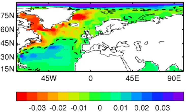
Figure 14.Regression (m Sv−1) of low frequency variations (69
years running means) in DSL anomaly against MOC, from the HadCM3 control simulation (1715 years). Dashed line shows the zero contour. Drift first removed (see Sect. 2).
against MOC strength (Fig. 14; which can be scaled to give the pattern for a 1 Sv decrease in MOC strength). The DSL changes from the MOC alone are only similar to that from the ice melt scenario (e.g. Fig. 5) in the Labrador Sea and central Arctic: they do not, however, match in the Greenland Sea or the central North Atlantic and NE Atlantic. Using the unforced control simulation, we constructed a year-to-year projection (π(t )in Eq. 1) of theunforcednorthern Atlantic DSL variations onto the forced ice scenario response pat-tern shown in Fig. 5a. A regression of this unforcedπ(t )on the corresponding unforced control MOC has a coefficient of −0.8 cm Sv−1. An ice-scenario-induced change to the MOC of about 1 Sv might thus contribute about 0.8 cm (under an assumption of linearity) of the ~2 cm change in the projec-tion parameter π(t) (Fig. 7): it is therefore not likely to be the sole contributor to the DSL change.
7 Summary and conclusions
We have used scenarios of projected 21st-century land-based ice melt to investigate the potential dynamical sea level re-sponse associated with ice melt alone. We have created two temporally and spatially varying data sets of land-ice melt over the 21st century, one a representative mid-range sce-nario and the other an illustrative high-end scesce-nario. The freshwater data sets include simulated melt from mountain glaciers and ice caps, and input from the major ice sheets. Both the ice sheet surface mass balance and dynamic changes are included, with a component associated with the partial collapse of the West Antarctic Ice Sheet making an appear-ance at the end of the 21st century in the high-end scenario. The scenarios are thus designed to represent potential time-lines of land-based freshwater flux into the ocean, rather than being sensitivity studies.
We have incorporated these ice sheet freshwater flux sce-narios into simulations using the HadCM3 model, with the
additional water inserted into the oceans at coastal grid cells. A simulation including global warming as well as the ice melt scenario shows a similar ice-melt pattern of DSL change from ice melt alone (in addition to the greater magnitude pat-tern associated with global warming) to that where the base-line conditions are pre-industrial. Despite the majority of the ice melt originating from Antarctica, the largest ice-scenario-induced changes in DSL are in the Arctic and the North At-lantic, with some lesser, but statistically significant, changes around Antarctica.
Our first conclusion is that for our model the mean ice-melt-related DSL change in the NW Atlantic is small com-pared, for example, to the DSL change which is typically seen in models forced by the A1B greenhouse gas scenario.
As we have noted, many previous studies have associated changes in North Atlantic DSL with changes in the MOC. Under our ice melt scenarios the effect of the additional freshwater flux on the MOC is small (<1 Sv). An analysis of the effect of such a low frequency change in MOC on north-ern Atlantic DSL pattnorth-ern, using a regression analysis of the long pre-industrial control simulation, suggests that∼60 % of the resultant DSL pattern is not associated with the MOC change and is likely to be more directly associated with the ice melt. This is our second conclusion.
Our third conclusion is that the pattern of ice-melt-related DSL change in our model is independent of the DSL change directly related to the warming scenario, and appears to scale according to the freshwater input. Consequently, the pat-tern of ice-melt-related DSL may be linearly added to other components such as those associated with heat uptake and changes to the hydrological cycle.
Acknowledgements. This work was supported by funding from the ice2sea programme from the European Union 7th Framework Programme, grant number 226375. Ice2sea contribution number #146. This work was also supported by the Joint UK DECC/Defra Met Office Hadley Centre Climate Programme (GA01101). The authors wish to express their gratitude to the referees whose comments helped to improve this article.
Edited by: A. Sterl
References
Aiken, C. M. and England, M. H.: Sensitivity of the present-day cli-mate to freshwater forcing associated with Antarctic sea ice loss, J. Climate, 21, 3936–3946, doi:10.1175/2007jcli1901.1, 2008. Baldwin, M. P., Stephenson, D. B., and Jolliffe, I. T.: Spatial
Weighting and Iterative Projection Methods for EOFs, J. Climate, 22, 2340–243, doi:10.1175/2008jcli2147.1, 2009.
Bevan, S. L., Luckman, A. J., and Murray, T.: Glacier dynamics over the last quarter of a century at Helheim, Kangerdlugssuaq and 14 other major Greenland outlet glaciers, The Cryosphere, 6, 923–937, doi:10.5194/tc-6-923-2012, 2012.
Bindschadler, R.: Hitting the Ice Sheets Where It Hurts, Science, 311, 1720–1721, doi:10.1126/science.1125226, 2006.
Bindschadler, R. A., Nowicki, S., Abe-Ouchi, A., Aschwanden, A., Choi, H., Fastook, J., Granzow, G., Greve, R., Gutowski, G., Herzfeld, U., Jackson, C., Johnson, J., Kroulev, C., Lever-mann, A., Lipsomb, W., Martin, M., Morlighem, M., Parizek, B., Pollard, D., Price, S., Ren, D., Saito, F., Sato, T., Seddik, H., Seroussi, H., Takahashi, K., Walker, R., and Wang, W. L.: Ice-sheet model sensitivities to environmental forcing and their use in projecting future sea level (the SeaRISE project), J. Glaciol., 59, 195–224, 2013.
Bingham, R. J. and Hughes, C. W.: Signature of the Atlantic meridional overturning circulation in sea level along the east coast of North America, Geophys. Res. Lett., 36, L02603, doi:10.1029/2008GL036215, 2009.
Christoffersen, P., Mugford, R. I., Heywood, K. J., Joughin, I., Dowdeswell, J. A., Syvitski, J. P. M., Luckman, A., and Ben-ham, T. J.: Warming of waters in an East Greenland fjord prior to glacier retreat: mechanisms and connection to large-scale atmo-spheric conditions, The Cryosphere, 5, 701–714, doi:10.5194/tc-5-701-2011, 2011.
Church, J. A., Woodworth, P. L., Aarup, T., and Wildon, W. S.: Un-derstanding Sea-Level Rise and Variability, 428 pp., 2010. Church, J. A., White, N. J., Konikow, L. F., Domingues, C. M.,
Cogley, J. G., Rignot, E., Gregory, J. M., van den Broeke, M. R., Monaghan, A. J., and Velicogna, I.: Revisiting the Earth’s sea-level and energy budgets from 1961 to 2008, Geophys. Res. Lett., 38, L18601, doi:10.1029/2011GL048794, 2011.
Church, J. A., Clark, P. U., Cazenave, A., Gregory, J. M., Jevrejeva, S., Levermann, A., Merrifield, M. A., Milne, G. A., Nerem, R. S., Nunn, P. D., Payne, A. J., Pfeffer, W. T., Stammer, D., and Un-nikrishnan, A. S.: Sea Level Change, in: Climate Change 2013: The Physical Science Basis. Contribution of Working Group I to the Fifth Assessment Report of the Intergovernmental Panel on Climate Change, edited by: Stocker, T. F., Qin, D., Plattner, G.-K., Tignor, M., Allen, S. G.-K., Boschung, J., Nauels, A., Xia, Y., Bex, V., and Midgley, P. M., Cambridge University Press, Cam-bridge, UK and New York, NY, USA, 13, 1137–1216, 2013. Cornford, S. L. Martin, D. F., Graves, D. T., Ranken, D. F.,
Le Brocq, A. M., Gladstone, R. M., Payne, A. J., Ng, E. G., and Lipscomb, W. H.: Adaptive mesh, finite volume mod-elling of marine ice sheets, J. Comput. Phys., 232, 529–549, doi:10.1016/j.jcp.2012.08.037, 2013.
Cunningham, S. A., Kanzow, T., Rayner, D., Baringer, M. O., Johns, W. E., Marotzke, J., Longworth, H. R., Grant, E. M., Hirschi, J. J. M., Beal, L. M., Meinen, C. S., and Bryden, H. L.: Temporal variability of the Atlantic meridional over-turning circulation at 26.5 degrees N, Science, 317, 935–938, doi:10.1126/science.1141304, 2007.
Doake, C. S. M. and Vaughan, D. G.: Rapid disintegration of the Wordie Ice Shelf in response to atmospheric warming, Nature 350, 328–330, doi:10.1038/350328a0, 1991.
Drijfhout, S. S., Weber, S. L., and van der Swaluw, E.: The stabil-ity of the MOC as diagnosed from model projections for
pre-industrial, present and future climates, Clim. Dynam., 37, 1575– 1586, doi:10.1007/s00382-010-0930-z, 2011.
Fettweis, X.: Reconstruction of the 1979–2006 Greenland ice sheet surface mass balance using the regional climate model MAR, The Cryosphere, 1, 21–40, doi:10.5194/tc-1-21-2007, 2007. Forster P. M. D. and Taylor K. E.: Climate forcings and climate
sensitivities diagnosed from coupled climate model integrations, J. Climate, 19, 6181–6194. doi:10.1175/jcli3974.1, 2006. Fürst, J. J., Goelzer, H., Huybrechts, P.: Effect of higher-order stress
gradients on the centennial mass evolution of the Greenland ice sheet, The Cryosphere, 7, 183–199, doi:10.5194/tc-7-183-2013, 2013.
Giesen, R. H. and Oerlemans, J.: Calibration of a surface mass balance model for global-scale applications, The Cryosphere, 6, 1463–1481, doi:10.5194/tc-6-1463-2012, 2012.
Giesen, R. H. and Oerlemans, J.: Climate-model induced dif-ferences in the 21st century global and regional glacier con-tributions to sea-level rise, Clim. Dynam., 41, 3283–3300, doi:10.1007/s00382-013-1743-7, 2013.
Gillet-Chaulet, F., Gagliardini, O., Seddik, H., Nodet, M., Du-rand, G., Ritz, C., Zwinger, T., Greve, R., and Vaughan, D. G.: Greenland ice sheet contribution to sea-level rise from a new-generation ice-sheet model, The Cryosphere, 6, 1561–1576, doi:10.5194/tc-6-1561-2012, 2012.
Gladstone, R. M., Bigg, G. R., and Nicholls, K. W.: Iceberg trajectory modeling and meltwater injection in the South-ern Ocean, J. Geophys. Res.-Ocean., 106, 19903–19915, doi:10.1029/2000jc000347, 2001.
Goelzer, H., Huybrechts, P., Fürst, J. J., Andersen, M. L., Edwards, T. L., Fettweis, X., Nick, F. M., Payne, A. J., and Shannon, S.: Sensitivity of Greenland ice sheet projections to model formu-lationsm, J. Glaciol., 59, 733–749, doi:10.3189/2013JoG12J182, 2013.
Gordon, C., Cooper, C., Senior, C. A., Banks, H., Gregory, J. M., Johns, T. C., Mitchell, J. F. B., and Wood, R. A.: The simulation of SST, sea ice extents and ocean heat transports in a version of the Hadley Centre coupled model without flux adjustments, Clim. Dynam., 16, 147–168, doi:10.1007/s003820050010, 2000. Graversen, R. G., Drijfhout, S., Hazeleger, W., van de Wal, R., Bin-tanja, R., and Helsen, M. Greenland’s contribution to global sea level rise by the end of the 21st century, Clim. Dynam., 37, 1427– 1442, 2011.
Gregory, J. M., Dixon, K. W., Stouffer, R. J., Weaver, A. J., Driesschaert, E., Eby, M., Fichefet, T., Hasumi, H., Hu, A., Jungclaus, J. H., Kamenkovich, I. V., Levermann, A., Mon-toya, M., Murakami, S., Nawrath, S., Oka, A., Sokolov, A. P., Thorpe, R. B.: A model intercomparison of changes in the At-lantic thermohaline circulation in response to increasing atmo-spheric CO2 concentration, Geophys. Res. Lett., 32, L12703, doi:10.1029/2005gl023209, 2005
Hakkinen, S. and Rhines, P. B.: Decline of subpolar North At-lantic circulation during the 1990s, Science, 304, 555–559, doi:10.1126/science.1094917, 2004.
with global climate forcing, J. Geophys. Res., 116, D24121, doi:10.1029/2011JD016387, 2011.
Hellmer, H. H., Kauker, F., Timmermann, R., Determann, J., and Rae, J.: Twenty-first-century warming of a large Antarctic ice-shelf cavity by a redirected coastal current, Nature, 485, 225– 228, doi:10.1038/nature11064, 2012.
Holland, D. M., Thomas, R. H., De Young, B., Ribergaard, M. H., and Lyberth, B.: Acceleration of Jakobshavn Isbrae triggered by warm subsurface ocean waters, Nature Geosci., 1, 659–664, doi:10.1038/ngeo316, 2008.
Howard, T., Pardaens, A. K., Bamber, J. L., Ridley, J., Spada, G., Hurkmans, R. T. W. L., Lowe, J. A., and Vaughan, D.: Sources of 21st century regional sea-level rise along the coast of northwest Europe, Ocean Sci., 10, 473–483, doi:10.5194/os-10-473-2014, 2014.
Hu, A. X., Meeh, G. A., Han, W. Q., and Yin, J. J.: Transient response of the MOC and climate to potential melting of the Greenland Ice Sheet in the 21st century, Geophys. Res. Lett. 36, L10707, doi:10.1029/2009GL037998, 2009.
Hu, A. X., Meehl, G. A., Han, W. Q., and Yin, J. J.: Effect of the potential melting of the Greenland Ice Sheet on the Meridional Overturning Circulation and global climate in the future, Deep-Sea Res., 58, 1914–1926, doi:10.1016/j.dsr2.2010.10.069, 2011. Hu, A. X., Meehl, G. A., Han, W. Q., Yin, J. J., Wu, B. Y., and Ki-moto, M.: Influence of Continental Ice Retreat on Future Global Climate, J. Climate, 26, 3087–3111, doi:10.1175/JCLI-D-12-00102.1, 2013.
IPCC: Special Report on Emissions Scenarios, edited by: Nakicen-ovic, N. and Swart, R., Cambridge University Press, UK, 570 pp., 2000.
Jackson, L. and Vellinga, M.: Multidecadal to Centennial Variability of the AMOC: HadCM3 and a Perturbed Physics Ensemble, J. Climate, 26, 2390–2407, doi:10.1175/JCLI-D-11-00601.1, 2013. Jacobs, S. S., Helmer, H. H., Doake, C. S. M., Jenkins, A., and Frolich, R. M.: Melting of Ice Shelves and the Mass Balance of Antarctica, J. Glaciol., 38, 375–387, 1992.
Keeling, R. F. and Visbeck, M.: On the Linkage between Antarc-tic Surface Water Stratification and Global Deep-Water Tem-perature, J. Clim., 24, 3545–3557, doi:10.1175/2011JCLI3642.1, 2011.
Kleinen, T., Osborn, T. J., and Briffa, K. R.: Sensitivity of climate response to variations in freshwater hosing location, Ocean Dy-nam., 59, 509–521, doi:10.1007/s10236-009-0189-2, 2009. Kopp, R. E., Mitrovica, J. X., Griffies, S. M., Yin, J. J., Hay, C. C.,
and Stouffer, R. J.: The impact of Greenland melt on local sea levels: a partially coupled analysis of dynamic and static equilib-rium effects in idealized water-hosing experiments A letter, Clim. Change, 103, 619–625, doi:10.1007/s10584.010.9935.1, 2010. Levermann, A. and Born, A.: Bistability of the Atlantic subpolar
gyre in a coarse-resolution climate model, Geophys. Res. Lett., 34, L24605, doi:10.1029/2007gl031732, 2007.
Levermann, A., Griesel, A., Hofmann, M., Montoya, M., and Rahmstorf, S.: Dynamic sea level changes following changes in the thermohaline circulation, Clim. Dynam., 24, 347–354, doi:10.1007/s00382-004-0505-y, 2005.
Levitus, S. R. and Boyer, T.: World Ocean Atlas 1994, Vol. 4: Temperature. NOAA Atlas NESDIS 4, US Gov. Printing Office, Washington DC, 117 pp., 1994.
Levitus, S. R., Burgett, T., and Boyer, T.: World Ocean Atlas 1994, Vol. 3: Salinity. NOAA Atlas NESDIS 3, US Gov. Printing Of-fice, Washington DC, 99 pp., 1994.
Livezey, R. E. and Chen, W. Y.: Statistical Field Significance and its Determination by Monte Carlo Techniques, Mon. Weather Rev., 111, 46–59, doi:10.1175/1520-0493(1983)111, 1983.
Lohmann, K., Drange, H., Bentsen, M.: Response of the North At-lantic subpolar gyre to persistent North AtAt-lantic oscillation like forcing, Clim. Dynam., 32, 273–285, doi:10.1007/s00382-008-0467-6, 2009.
Lorbacher, K., Dengg, J., Böning, C. W., and Biastoch, A.: Re-gional Patterns of Sea Level Change Related to Interannual Variability and Multidecadal Trends in the Atlantic Merid-ional Overturning Circulation*, J. Climate, 23, 4243–4254, doi:10.1175/2010JCLI3341.1, 2010.
Lorbacher, K., Marsland, S. J., Church, J. A., Griffies, S. M., and Stammer, D.: Rapid barotropic sea level rise from ice sheet melt-ing, J. Geophys. Res., 117, C06003, doi:10.1029/2011JC007733, 2012.
Lowe, J. A. and Gregory, J. M.: Understanding projections of sea level rise in a Hadley Centre coupled climate model, J. Geophys. Res.-Ocean., 111, C11014, doi:10.1029/2005JC003421, 2006. Lowe, J. A., Howard, T. P., Pardaens, A., Tinker, J., Holt, J.,
Wake-lin, S., Milne, G., Leake J., Wolf, J., Horsburgh, K., Reeder, T., Jenkins, G., Ridley, J., Dye, S., and Bradley, S. UK Cli-mate Projections science report: Marine and coastal projections. Met Office Hadley Centre, Exeter, UK. Copies available to order or download from: http://ukclimateprojections.defra.gov.uk (last access: 20 December 2012), 2009.
Marzeion, B., Jarosch, A. H., and Hofer, M.: Past and future sea-level change from the surface mass balance of glaciers, The Cryosphere, 6, 1295–1322. doi:10.5194/tc-6-1295-2012, 2012. McGrath, D., Steffen, K., Rajaram, H., Scambos, T.,
Ab-dalati, W., and Rignot, E.: Basal crevasses on the Larsen C Ice Shelf, Antarctica: Implications for meltwater pond-ing and hydrofracture, Geophys. Res. Lett., 39, L16504, doi:10.1029/2012GL052413.
Meehl, G. A., Stocker, T. F., Collins, W. D., Friedlingstein, P., Gaye, A. T., Gregory, J. M., Kitoh, A., Knutti, R., Murphy, J. M., Noda, A., Raper, S. C. B., Watterson, I. G., Weaver, A. J., and Zhao, Z.: Global climate projections, edited by: Solomon, S., Qin, D., Manning, M., Chen, Z., Marquis, M., Averyt, K. B., Tignor, M., Miller, H. L., Climate change 2007: The Physical Science Ba-sis. Contribution of Working Group I to the Fourth Assessment Report of the Intergovernmental Panel on Climate Change, Cam-bridge University Press, London, 2007.
Meier, M. F. and Post, A.: Fast tidewater glaciers, J. Geophys. Res., 92, 9051–9058, doi:10.1029/JB092iB09p09051, 1987.
Meier, M. F., Dyurgerov, M. B., Rick, U. K., O’Neel, S., Pfeffer, W. T., Anderson, R. S., Anderson, S. P., and Glazovsky, A. F.: Glaciers dominate eustatic sea-level rise in the 21st century, Sci-ence 317, 1064–1067, doi:10.1126/sciSci-ence.1143906, 2007. Mikolajewicz, U., Vizcaino, M., Jungclaus, J., and Schurgers,
G.: Effect of ice sheet interactions in anthropogenic cli-mate change simulations, Geophys. Res. Lett., 34, L18706, doi:10.1029/2007gl031173, 2007.
Mitrovica, J. X., Tamisiea, M. E., Davis, J. L., and Milne, G. A.: Recent mass balance of polar ice sheets inferred from patterns of global sea-level change. Nature 409, 1026–1029, doi:10.1038/35059054, 2001.
Nicholls, R. J., Marinova, N., Lowe, J. A., Brown, S., Vellinga, P., De Gusmao, D., Hinkel, J., and Tol, R. S. J.: Sea-level rise and its possible impacts given a ’beyond 4 degrees C world’ in the twenty-first century, Philos. Trans. Roy. Soc., 369, 161–181, doi:10.1098/rsta.2010.0291, 2011.
Nick, F. M., Vieli, A., Andersen, M. L., Joughin, I. R., Payne, A. J., Edwards, T., Pattyn, F., and van der Wal, R.: Future sea level rise from Greenland’s major outlet glaciers in a warming climate, Nature, 497, 235–238, 2013.
Nowicki, S., Bindschadler, R., Abe-Ouchi, A., Aschwanden, A., Bueler, E., Choi, H., Fastook, J., Granzow, G., Greve, R., Gutowski, G., Herzfeld, U., Jackson, C., Johnson, J., Kroulev, C., Larour, E., Levermann, A., Lipsomb, W., Martin, M., Morlighem, M., Parizek, B., Pollard, D., Price, S., Rignot, E., Ren, D., Saito, F., Sato, T., Seddik, H., Seroussi, H., Takahashi, K., Walker, R., and Wang, W. L.: Insights into spatial sensitivities of ice mass response to environmental change from the SeaRISE ice sheet modeling project I. Antarctica, J. Geophys. Res., 118, 1002–1024, 2013a.
Nowicki, S., Bindschadler, R., Abe-Ouchi, A., Aschwanden, A., Bueler, E., Choi, H., Fastook, J., Granzow, G., Greve, R., Gutowski, G., Herzfeld, U., Jackson, C., Johnson, J., Kroulev, C., Larour, E., Levermann, A., Lipsomb, W., Martin, M., Morlighem, M., Parizek, B., Pollard, D., Price, S., Rignot, E., Ren, D., Saito, F., Sato, T., Seddik, H., Seroussi, H., Takahashi, K., Walker, R., and Wang, W. L.: Insights into spatial sensitivities of ice mass response to environmental change from the SeaRISE ice sheet modeling project II. Greenland, J. Geophys. Res., 118, 1025–1044, 2013b.
Pardaens, A. K., Banks, H. T., Gregory, J. M., and Rowntree, P. R.: Freshwater transports in HadCM3. Climate Dynamics 21, 177– 195, doi:10.1007/s00382-003-0324-6, 2003.
Pardaens, A. K., Gregory, J. M., and Lowe, J. A.: A model study of factors influencing projected changes in regional sea level over the twenty-first century, Clim. Dynam., 36, 2015–2033, doi:10.1007/s00382-009-0738-x, 2011.
Pattyn, F., Schoof, C., Perichon, L., Hindmarsh, R. C. A., Bueler, E., de Fleurian, B., Durand, G., Gagliardini, O., Gladstone, R., Gold-berg, D., Gudmundsson, G. H., Huybrechtsm P., Lee, V., Nick, F. M., Payne, A. J., Pollard, D., Rybak, O., Saito, F., and Vieli, A. () Results of the Marine Ice Sheet Model Intercomparison Project, MISMIP, The Cryosphere, 6, 573–588, doi:10.5194/tc-6-573-2012, 2012.
Pfeffer, W. T., Harper, J. T., and O’Neel S.: Kinematic constraints on glacier contributions to 21st-century sea-level rise, Science, 321, 1340–1343, doi:10.1126/science.1159099, 2008.
Pope, V. D., Gallani, M. L., Rowntree, P. R., and Stratton, R. A.: The impact of new physical parametrizations in the Hadley Centre climate model: HadAM3, Clim. Dynam., 16, 123–146, doi:10.1007/s003820050009, 2000.
Price, S. F., Payne, A. J., Howat, I. M., and Smith, B. E.: Committed sea-level rise for the next century from Greenland ice sheet dy-namics during the past decade, Proc. Natl. Acad. Sci. USA, 108, 8978–8983, doi:10.1073/pnas.1017313108, 2011.
Pritchard, H. D., Arthern, R. J., Vaughan, D. G., and Edwards, L. A.: Extensive dynamic thinning on the margins of the Greenland and Antarctic ice sheets, Nature, 461, 971–975, doi:10.1038/nature08471, 2009.
Pritchard, H. D., Ligtenberg, S. R. M., Fricker, H. A., Vaughan, D. G., van den Broeke, M. R., and Padman, L.: Antarctic ice-sheet loss driven by basal melting of ice shelves, Nature, 484, 502–505, doi:10.1038/nature10968, 2012.
Radic, V. and Hock, R.: Regionally differentiated contribution of mountain glaciers and ice caps to future sea-level rise, Nature Geosci., 4, 91–94, doi:10.1038/ngeo1052, 2011.
Rahmstorf, S.: On the freshwater forcing and transport of the At-lantic thermohaline circulation, Clim. Dynam., 12, 799–811, doi:10.1007/s003820050144, 1996.
Rayner, N. A., Parker, D. E., Horton, E. B., Folland, C. K., Alexan-der, L. V., Rowell, D. P., Kent, E. C., and Kaplan, A.: Global analyses of sea surface temperature, sea ice, and night marine air temperature since the late nineteenth century, J. Geophys. Res.-Atmos., 108, 4407, doi:10.1029/2002jd002670, 2003.
Richardson, G., Wadley, M. R., Heywood, K. J., Stevens, D. P., and Banks, H. T.: Short-term climate response to a freshwater pulse in the Southern Ocean, Geophys. Res. Lett., 32, L03702, doi:10.1029/2004GL021586, 2005.
Ridley, J. K., Huybrechts, P., Gregory, J. M., and Lowe, J. A.: Elim-ination of the Greenland ice sheet in a high CO2climate, J.
Cli-mate, 18, 3409–3427, doi:10.1175/jcli3482.1, 2005.
Ritz, C., Durand, G., Edwards, T. L., Payne, A. J., Peyaud, V., Richard, C. A., Hindmarsh, R. C. A.: Bimodal probability of the dynamic contribution of Antarctica to future sea level, Nature, 2014.
Roeckner, E., Brokopf, R., Esch, M., Giorgetta, M., Hagemann, S., Kornblueh, L., Manzini, E., Schlese, U., and Schulzweida, U.: Sensitivity of simulated climate to horizontal and vertical reso-lution in the ECHAM5 atmosphere model, J. Climate, 19, 3771– 3791, 2006.
Russell, G. L., Gornitz, V., and Miller, J. R.: Re-gional sea level changes projected by the NASA/GISS Atmosphere-Ocean Model, Clim. Dynam., 16, 789–797, doi:10.1007/s003820000090, 2000.
Schmittner, A., Latif, M., and Schneider, B.: Model projections of the North Atlantic thermohaline circulation for the 21st cen-tury assessed by observations, Geophys. Res. Lett., 32, L23710, doi:10.1029/2005GL024368, 2005.
Schoof, C.: Marine ice-sheet dynamics. Part 1. The case of rapid sliding. J. Fluid Mechan., 573, 27–55, doi:10.1017/s0022112006003570, 2007.
Seddik, H., Greve, R., Zwinger, T., Gillet-Chaulet, F., and Gagliar-dini, O.: Simulations of the Greenland ice sheet 100 years into the future with the full Stokes model Elmer/Ice, J. Glaciol., 58, 427–440, doi:10.3189/2012JOG11J177, 2012.
Spada, G., Bamber, J. L., Huurkmans, R.: The gravitationally-consistent fingerprint of future terrestrial ice loss, Geophys. Res. Lett., 40, 482–486, doi:10.1029/2012GL053000, 2013. Stammer, D.: Response of the global ocean to Greenland and
Antarctic ice melting, J. Geophys. Res.-Ocean., 113, C06022, doi:10.1029/2006jc004079, 2008.
to Greenland Ice Melting, Surv. Geophys., 32, 621–642, doi:10.1007/s10712-011-9142-2, 2011.
Stanton, T. P., Shaw, W. J., Truffer, M., Corr, H. F. J., Peters, L. E., Riverman, K. L., Bindschadler, R., Holland, D. M., and Anan-dakrishnan, S.: Channelized Ice Melting in the Ocean Bound-ary Layer Beneath Pine Island Glacier, Antarctica, Science, 341, 1236–1239, doi:10.1126/science.1239373, 2013.
Stouffer, R. J., Seidov, D., and Haupt, B. J.: Climate response to ex-ternal sources of freshwater: North Atlantic versus the Southern Ocean, J. Climate, 20, 436–448, doi:10.1175/jcli4015.1, 2007. Stouffer, R. J., Yin, J., Gregory, J. M., Dixon, K. W., Spelman, M.
J., Hurlin, W., Weaver, A. J., Eby, M., Flato, G. M., Hasumi, H., Hu, A., Jungclaus, J. H., Kamenkovich, I. V., Levermann, A., Montoya, M., Murakami, S., Nawrath, S., Oka, A., Peltier, W. R., Robitaille, D. Y., Sokolov, A., Vettoretti, G., and Weber, S. L.: Investigating the causes of the response of the thermohaline circulation to past and future climate changes, J. Climate, 19, 1365–1387. doi:10.1175/jcli3689.1, 2006.
Swingedouw, D., Fichefet, T., Huybrechts, P., Goosse, H., Driess-chaert, E., and Loutre, M.-F.: Antarctic ice-sheet melting pro-vides negative feedbacks on future climate warming, Geophys. Res. Lett., 35, L17705, doi:10.1029/2008GL034410, 2008. Swingedouw, D., Fichefet, T., Goosse, H., Loutre, M. F.:
Im-pact of transient freshwater releases in the Southern Ocean on the AMOC and climate, Climate Dynam., 33, 365–381, doi:10.1007/s00382-008-0496-1, 2009.
Swingedouw, D., Rodehacke, C. B., Behrens, E., Menary, M., Olsen, S. M., Gao, Y., Mikolajewicz, U., Mignot, J., and Bi-astoch, A.: Decadal fingerprints of freshwater discharge around Greenland in a multi-model ensemble, Clim. Dynam., 41, 695– 720, doi:10.1007/s00382-012-1479-9, 2013.
Timmermann, R., Wang, Q., and Hellmer, H. H.: Ice-shelf basal melting in a global finite-element sea-ice/ice-shelf/ocean model, Ann. Glaciol., 53, 303–314, doi:10.3189/2012AoG60A156, 2012.
Van den Broeke, M. R., Bamber, J., Lenaerts, J., and Rignot, E.: Ice Sheets and Sea Level: Thinking Outside the Box, Surv. Geo-phys., 32, 495–505, doi:10.1007/s10712-011-9137-z, 2011. Vellinga, M. and Wu, P. L.: Low-latitude freshwater influence on
centennial variability of the Atlantic thermohaline circulation, J. Climate 17, 4498–4511, doi:10.1175/3219.1, 2004.
Wang, X., Wang, Q. Sidorenko, D., Danilov, S., Schroter, J., and Jung, T.: Long-term ocean simulations in FESOM: evaluation and application in studying the impact of Greenland Ice Sheet melting, Ocean Dynam., 62, 1471–1486, doi:10.1007/s10236-012-0572-2, 2012.
Weaver, A. J., Sedláˇcek, J., Eby, M., Alexander, K., Crespin, E., Fichefet, T., Gwenaëlle P., Joos, F., Kawamiya, M., Matsumoto, K., Steinacher, M., Tachiiri, K., Tokos, K., Yoshimori, M., and Zickfeld, K.: Stability of the Atlantic meridional overturning circulation: A model intercomparison, Geophys. Res. Lett., 39, L20709, doi:10.1029/2012GL053763, 2012.
Weaver, A. J., Saenko, O. A., Clark, P. U., Mitrovica, J. X.: Meltwater pulse 1A from Antarctica as a trigger of the Bolling-Allerod warm interval, Science, 299, 1709–1713 doi:10.1126/science.1081002, 2003.
Yin, J. J., Schlesinger, M. E., and Stouffer, R. J.: Model projections of rapid sea-level rise on the northeast coast of the United States, Nature Geosci., 2, 262–266, doi:10.1038/ngeo462, 2009. Yin, J.: Century to multi-century sea level rise projections