Annales
Geophysicae
An assessment of the “map-potential” and “beam-swinging”
techniques for measuring the ionospheric convection pattern using
data from the SuperDARN radars
G. Provan1, T. K. Yeoman1, S. E. Milan1, J. M. Ruohoniemi2, and R. Barnes2
1Department of Physics and Astronomy, University of Leicester, University Road, Leicester LE1 7RH, UK 2Applied Physics Laboratory, John Hopkins University, Laurel, Maryland, USA
Received: 19 February 2001 – Revised: 1 October 2001 – Accepted: 3 October 2001
Abstract. The SuperDARN HF coherent scatter radars (Greenwald et al., 1995) provide line-of-sight (l-o-s) velocity measurements of ionospheric convection flow over the polar regions of the northern and southern hemispheres. A num-ber of techniques have been developed in order to obtain 2-D plasma flow vectors from these l-o-s observations. This study entails a comparison of the ionospheric flow vectors de-rived using the “map-potential”, and “beam-swinging” niques with the vectors derived using the “merging” tech-nique. The merging technique is assumed to be the most ac-curate method of deriving local flow vectors from l-o-s veloc-ities. We can conclude that the map-potential model is signif-icantly more successful than the beam-swinging technique at estimating both the magnitude and the direction of the large-scale ionospheric convection flow vectors. The quality of the fit is dependent on time of day, with vectors observed at low latitudes in the dawn sector agreeing most closely with the merged vector flow pattern.
Key words. Ionosphere (plasma convection; instruments and techniques) – Radio science (instruments and tech-niques)
1 Introduction
Coherent scatter radars have provided measurements of iono-spheric convection for almost thirty years. Individually, such radars make l-o-s (l-o-s) velocity measurements of the plasma flow in the radar look direction. In the past, three VHF coherent radars, the Scandinavian Twin Auroral Radar Experiment (STARE) (Greenwald et al., 1978), the Sweden and Britain Radar-auroral Experiment (SABRE) (Nielsen et al., 1983) and the Bistatic Auroral Radar System (BARS) (Andr´e et al., 1988), have calculated “true” bistatic merged vectors by combining l-o-s vectors obtained from different radars with overlapping fields-of-view. However, any mea-surement of E-region irregularities made by these VHF
co-Correspondence to:G. Provan ([email protected])
herent radars is limited to the ion acoustic speed (Nielsen and Schlegel, 1983, 1985; Kofman and Nielsen, 1990) al-though this speed will increase nonlinearly with plasma drift velocity (Robinson, 1986). Subsequently, the F-region of the ionosphere was studied by the Polar Anglo-American Con-jugate Experiment (PACE) at Goose Bay and Halley (Ruo-honiemi et al., 1989). These single radars could only provide the l-o-s velocity component of the plasma motion, as the in-dividual radar fields-of-view do not overlap. For the PACE radars the transverse velocity component was obtained using data from these single radars by a beam-swinging technique (Villain et al., 1987; Ruohoniemi et al., 1987; 1989). Yeo-man et al. (1992) assessed the beam-swinging technique as used to study E-region irregularity drift patterns with data from the SABRE radars. They found that both curvature and gradient in the flow vectors will cause errors in the velocity estimates, with 30% or more of the beam-swinging derived velocities lying outside a cone of half-width 30◦around the merged SABRE drift velocities. Freeman et al. (1991) stud-ied vectors derived from the beam-swinging technique us-ing a simulation of a 16-beam, sus-ingle-station radar, compar-ing the simulation results with the results expected from a two-beam radar model. They found that although large-scale flows were in general reproduced well, curvature of the flow resulted in error in the beam-swung derived vectors, espe-cially if the radius of the curvature of the flow structure had a scale size equal to, or less than, the radar field-of-view.
irregulari-W
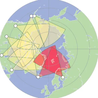
Fig. 1.The fields-of-view of the Northern hemisphere SuperDARN radars. The CUTLASS radars at Pykkvibær and Hankasalmi are shaded red.
ties, the velocity of the F-region irregularities is not limited by the sound speed of the plasma, but moves with the con-vectiveE×Bambient plasma drift velocity. Thus the 2-D merged vectors obtained from the HF radars can serve to map the plasma convection.
Merging relies on two or more radars having overlapping fields-of-view and observing backscatter simultaneously at the same position. A great portion of the fields-of-view of the radar systems is viewed by one radar only and, even where the radar fields-of-view do overlap, it is not uncom-mon for one radar to observe backscatter and not the other. The data, which cannot be used directly to provide merged vectors, can still provide a wealth of information about the ionospheric flows. In response to this the “map-potential” model (Ruohoniemi and Baker, 1998) was developed, aim-ing to utilize all available data from the SuperDARN radars to deduce the global convection pattern. As yet, the fields-of-view of the SuperDARN radars do not have global cover-age and the operating radars do not observe backscatter at all range gates at all times. To deduce a global convection pat-tern, the observed l-o-s velocities from all the SuperDARN radars have to be combined with data from a statistical model (Ruohoniemi and Greenwald, 1996), to produce “fitted” flow vectors and a global convection model that is in best agree-ment with the observed l-o-s velocities.
The map-potential technique is becoming the standard technique for determining global ionospheric flow; no work assessing its accuracy has yet been published, however. This paper involves a statistical study using data from the CUT-LASS HF bistatic coherent scatter radars at Hankasalmi, Fin-land and Pykkvibær, IceFin-land (part of the SuperDARN
net-work of HF radars), to assess the flow vectors derived by both the beam-swinging technique and the map-potential model, with the 2-DE×Bdrift velocities obtained by directly merg-ing velocity measurements from the two radar systems, in or-der to quantitatively assess the accuracy of the map-potential technique and compare it with the beam-swinging method. Here we use the 1998 map-potential technique; however sev-eral improvements have been made to the technique since that time (Shepherd and Ruohoniemi, 2000). A perfect agreement between the vectors derived by the merging and map-potential techniques is not expected due to HF noise and misidentified ground scatter contaminating the l-o-s velocity data. Such noise can usually be identified in a case study but not in a large statistical study. There is also a difference in the applicability of the merge and the map-potential tech-nique. The merging technique aims to derive the optimum local solution. The map-potential technique derives large-scale solutions, with the data being median filtered before being “fitted” to a spherical harmonic expansion of the elec-trostatic potential (see Sect. 2.3). Thus the merging technique can show sources and sinks in the flow; this behaviour is not consistent with a potential solution, however.
2 Data and data analysis techniques
2.1 Instrumentation
The intention of the present study is to assess the accu-racy of the beam-swinging technique and the map-potential model in estimating 2-D flow vectors of ionospheric irregu-larities, these irregularities moving at the convectiveE×B drift velocity over an extended region of the high-latitude ionosphere. The measured drift velocity vectors are esti-mated on the basis of bistatic coherent HF radar measure-ments provided by the SuperDARN radars at Hankasalmi and Pykkvibær. The phase velocity of irregularity drifts detected at HF, which is measured primarily in the F-region at heights of 150–600 km, is dominated by the contribution from the large-scale drifts of the ambient plasma driven, for example, by the gradient drift instability (Fejer and Kelley, 1980), and should not differ substantially from theE×Bdrift velocity (Villain et al., 1985; Ruohoniemi et al., 1987; Davies et al., 1999, 2000).
52◦in azimuth and over 3000 km in range (an area of over
4×10⁶km2), every 1 or 2 min. Common-volume data from the two stations can be combined to provide convection ve-locities perpendicular to the magnetic field. This dataset is supplemented by upstream IMF data from the WIND satel-lite (Lepping et al., 1995).
2.2 Merging
The northern hemisphere SuperDARN radars are arranged in 6 radar pairs, each pair allowing simultaneous l-o-s plasma drift measurements from two different directions in a com-mon field-of-view. As each radar sounds along 16 beams, a 16×16 grid of overlapping measurements is available from each pair. These measurements can be combined, using a process called “merging”, to provide a maximum of 256 2-D plasma flow vectors per-radar-pair. Under optimum condi-tions, direct mapping of ionospheric convection in the North-ern hemisphere can be extended to more than 12 h of MLT. In practice, backscatter is not available within all merge cells and fewer than the maximum 256 vectors per-radar-pair are calculated (Hanuise et al., 1993).
2.3 The map-potential model
In an effort to improve the coverage available from the merge technique the “map-potential” technique, was developed by Ruohoniemi and Baker (1998). The authors argued that, even if merged vectors cannot be determined due to poor cover-age from one of a pair of radar fields-of-view, all the avail-able l-o-s velocities serve to constrain the possibilities for the large-scale convection velocity. The convection pattern that is most consistent with the measurements can be deter-mined by a mathematical fitting technique involving all the available l-o-s data. This is the basis for the map-potential technique, described by Ruohoniemi and Baker (1998) as “a method of filtering, combining and reducing data from the SuperDARN radars which optimizes the fitting of large-scale convection patterns”. This philosophy is similar to the approach taken in the derivation of some statistical convec-tion models (i.e. Ruohoniemi and Greenwald, 1996; Weimer, 1995) and by the assimilative mapping of electrodynamics (AMIE) procedure (Richmond and Kamide, 1988).
Initially the l-o-s velocity data from each radar are filtered by performing a “boxcar” filter involving both spatial and temporal filtering. The smoothed data is then mapped onto a global grid which is 1◦ in latitude (approx. 111 km pro-jected onto the surface of the Earth) and as close as possible to 111 km in longitude. The gridded data from each radar is then combined into a single file, using a temporal averaging period which can be as short as the scan repetition rate. The combined l-o-s velocity data for a period is then “fitted” to an expansion of the electrostatic potential in spherical harmonic functions (e.g. Jackson, 1962; Ruohoniemi and Baker, 1998; Bristow et al, 1998).
The solution is constrained by folding in information from a statistical model (Ruohoniemi and Greenwald, 1996),
SUPERDARN PARAMETER PLOT
Beamswung vectors vectors
25 Feb 1998
1630 - 1632
-400 -300 -200 -100 0 100 200 300 400
V
elocity (ms
-1
)
Ground Scatter
1000 ms-1
1630 - 1632
-400 -300 -200 -100 0 100 200 300 400
V
elocity (ms
-1
)
Ground Scatter Merged vectors
(a)
(b)
1000 ms-1
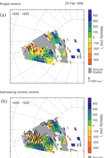
Fig. 2. (a)Polar plot of l-o-s velocities detected by the Hankasalmi radar on 25 February 1998, 16:30 UT. The velocity is colour coded with red (negative) velocities indicating motion away from the radar and blue/green (positive) velocities indicating motion toward the radar. Overlayed are merged vectors calculated using l-o-s veloci-ties from the Hankasalmi and Pykkvibær radars for the same period.
(b)Polar plot of l-o-s velocities detected by the Hankasalmi radar on 25 February 1998, 16:30 UT (as in Fig. 2a). Overlayed are beam-swung vectors calculated using l-o-s velocities from the Hankasalmi radar for the same period.
keyed to the IMF conditions. The orderland degreemof the expansion determine the spatial filtering performed on the velocity data. In this statistical study we usel =m=4 for all days. In the map-potential technique, as the order of the fitting is increased, the statistical model is sampled at more points to constrain the additional terms of the expansion but the weight assigned to each of the samples is reduced in in-verse proportion. In this way the ‘effective’ contribution of the statistical model to the “fitted” solution does not increase with order (Shepherd and Ruohoniemi, 2000).
types of velocity flow vectors; in this study we are concerned with two of these. “Fitted” vectors are produced which rep-resent the l-o-s velocity vectors which have been “fitted” to the global convection pattern. “True” vectors are also pro-duced by combining the transverse component of the “fit-ted” velocity vectors with the measured l-o-s velocity, thus allowing the small-scale variations of the l-o-s velocity to be recovered. Several quality-of-fit parameters are also ob-tained from the “fitting” procedure, including the “reduced” chi-squared (χr2) obtained by dividingχ2by the number of degrees of freedom in the fitting. If the measurements are physical (i.e. can be represented as the gradient of a scalar potential) and the measurements are distributed normally,χr2
gauges the degree to which the distribution of the offsets (i.e. the differences between the “fitted” and measured velocities) is consistent with the uncertainties assigned to the measure-ments (Ruohoniemi and Baker, 1998).
2.4 The beam-swinging technique
The l-o-s velocity measured by a single radar beam provides only one component of the plasma flow. When measure-ments from several beams are combined it is possible to es-timate the flow component perpendicular to the radar beam and thus derive the magnitude and angle of the plasma flow. This is the basis of “beam-swinging”, a technique first devel-oped in the 1960s. The beam-swinging technique used here attempts to derive a value for the transverse velocity com-ponent, Vφ, by assuming that the flow along a contour of
constant L-shell is constant with respect to the L-shell; thus the l-o-s velocity varies simply as a cosine of the angle that the radar look direction makes with the L-shell contour. This assumption was first described by Ruohoniemi et al. (1989). It is described by Eq. (1), whereVflowis the velocity at which the plasma is flowing at an azimuthal angleθflow. If the flow is observed by a radar beam located at an angleθradarto the L-shell, the observed l-o-s velocity,Vl-o-s, is given by Vl-o-s=Vflowcos(θradar−θflow) (1) L-o-s velocities observed by any number of radar beams can be used to determine the flow along a particular L-shell. The obtained vectors are resolved into components parallel and perpendicular to the radar look direction over the full field-of-view of the radar. The derived perpendicular component is then combined with the measured parallel (line-of-sight) component to produce a corrected vector. This allows the small-scale variations of the l-o-s velocity to be recovered af-ter the smoothing effects of the large-scale L-shell fits. From here, on this process will be referred as “beam-swinging” and the product as “beam-swung velocities”.
3 The statistical study
In this study we compare vectors derived by the beam-swinging and map-potential techniques with vectors derived using the merging algorithm. The merged vectors are as-sumed to be the most accurate, as these vectors are based
purely on radar observations and no prior assumptions are made when deriving them. The statistical database for this study comprises 164 days of data from 1998 when the CUT-LASS radars were run in normal mode (operating all 16 beams with 2 min resolution and 45 km range gates) for the entire day. We merged the l-o-s velocity data from the two radars for all the selected days, resulting in a to-tal of∼145 000 merged data points, which form the basis for our statistical study. Figure 2 illustrates an example of the radar scan, showing Hankasalmi l-o-s velocities obtained from the 25 February 1998, 16:30 to 16:32 UT. L-o-s veloc-ity is colour coded with negative velocities (red/yellow) rep-resenting flow away from the radar and positive velocities (blue/green) representing flows towards the radar. Overlaid on the l-o-s velocity are merged velocity vectors obtained by merging data for the Hankasalmi and Pykkvibær radars from the same period.
Beam-swung vectors were obtained from the l-o-s veloc-ity data observed by the Finland radar using the method out-lined in Sect. 2.4. Each L-shell in the beam-swinging al-gorithm was 2◦wide and the beam-swinging algorithm was only performed if there were three or more data points in any given L-shell. The error of the velocity magnitude of every beam-swung vector was calculated for each L-shell. Figure 2b shows the beam-swung vectors obtained for the 25 February 1998, 16:30 to 16:32 UT. For the statistical study we compared each merged data point with its nearest beam-swung data point.
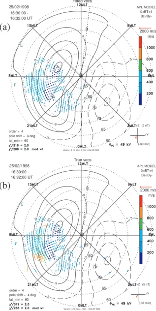
L-o-s velocity data from the Hankasalmi and Pykkvibær radars were used to obtain 2-D flow vectors using the map-potential model described in Sect. 2.3. Both “fitted” and “true” 2-D flow vectors were obtained for each 2 min scan of the 164 days of the statistical study. The statistical model, which forms part of the map-potential routine, is dependent on the prevailing IMF conditions. Data from the WIND satel-lite was used to measure the daily IMF conditions, the delay time between when the solar wind reaches the satellite and when it impinges on the subsolar magnetopause was calcu-lated using the method of Lester et al. (1993). Figure 3a presents the “fitted” vectors calculated using data from the Hankasalmi radar for 25 February 1998 at 16:30 UT, while Fig. 3b shows the “true” vectors for the same period. Again, for the statistical study we compared each merged vector with its nearest vector as calculated by the map-potential model.
4 Results of the statistical comparison
0 0
60 65 70 75 80 85 90
E
F
-21 -21
-9
-9
-9
-9
3
3
3
15
APL MODEL 0<BT<4
Fitted vecs 25/02/1998
16:30:00 -16:32:00 UT
2000 m/s m/s
order = 4 pole shift = 4 deg lat_min = 60
+Y +Z (5 nT)
(-63 min) Version: 4.10 Mon, 2 Oct,14:04:28 2000
0 0
60 65 70 75 80 85 90
E
F
-21 -21
-9
-9
-9
-9
3
3
3
15
APL MODEL 0<BT<4
True vecs 25/02/1998
16:30:00 -16:32:00 UT
2000 m/s m/s
order = 4 pole shift = 4 deg lat_min = 60
+Y +Z (5 nT)
(-63 min) Version: 4.10 Mon, 2 Oct, 14:06:07 2000
(a)
(b)
Fig. 3. (a)“Fitted” map-potential vectors for 25 February 1998, 16:30 to 16:32 UT. The velocity data are scaled to the length of the reference arrow and are also colour-coded by magnitude. Solid (dotted) contours are associated with negative (positive) values of the electrostatic potential, and the contour interval is 6 kV. The vectors are obtained by fitting the l-o-s velocity data and data from a statistical convection pattern to a low-order expansion (L=4) of the electrostatic potential in spherical harmonics. The predictions of the statistical convection model are based on the prevailing IMF conditions, with IMF measurements being made by the WIND spacecraft. A schematic of the IMF vectors in the GSMY−Zplane is shown in the bottom right hand corner. There is a 63 min delay time between detection of the solar wind by the WIND spacecraft and its impingement on the subsolar magnetopause.(b)“True” map-potential vectors for 25 February 1998, 16:30 to 16:32 UT
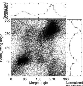
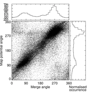
The normalized occurrence distribution of the angles sured by both techniques is also shown. Angles are mea-sured clockwise from geomagnetic north. In all cases the 45◦ line represents the idealized case where the beam-swinging technique perfectly reproduces the merged velocity direction measurements. The velocity direction plot shows two dis-tinct clusters of points. One cluster is around 90◦, due to eastward flow measured by the radar in the dawn convec-tion cell; the other cluster is around 270◦, due to westward flow in the dusk convection cell. This clustering is due to the beam-swinging technique assuming the plasma flow to
Table 1.A comparison of velocity direction calculated using the beam-swung and map-potential techniques with the velocity direction of merged vectors
Velocity direction % within 45◦cone
of merged angles
All beam-swung angles 48
Beam-swung angles with rms error<150 m/s 61
All fitted map-potential angles 65
Fitted map-potential angles withχ2<1.5 64
All true map-potential angles 66
Beam-swung vectors observed at dusk between 65◦and 70◦magnetic lat. 75 True map-potential observed at midday between 65◦and 70◦magnetic lat. 84
0 90 180 270 360
Merge angle 0
90 180 270 360
Beam_swing angle
Normalised occurrence
Normalised occurrence Comparison between merged and
beam_swung angles
Total number of data points 143401.
Fig. 4.Comparison between merged and beam-swung velocity di-rections. Also shown are the normalized occurrence distributions of the angles.
to the dawn sector peak (7047 data points). In general, the two clusters of points show a greater range in the velocity direction determined by the merging algorithm than by the beam-swinging technique, especially in the flow measured in the dawn convection cell.
Table 1 summarises the results of the statistical compari-son between vector direction calculated by the various tech-niques in this study. 48% of beam-swung derived veloc-ity directions lie inside a cone of 45◦half-width around the merged velocity estimates. When beam-swung data points which have been filtered, so that only the data points which have an rms error in their velocity magnitude of 15 m/s or less
0 200 400 600 800 1000
Merge velocity 0
200 400 600 800 1000
Beam_swung velocity
0 200 400 600 800 1000
Merge velocity 0
200 400 600 800 1000
Beam_swung velocity
Comparison between merged and beam_swung velocities
0.0 0.2 0.4 0.6 0.8 1.0
Normalised colour scale
Fig. 5. Comparison between merged and beam-swung velocity magnitudes. The normalized occurrence distribution of data points is colour coded with red indication region of most data points and blue indication region of fewest data points.
(compared to the best-fit velocity measured at that L-shell), then 61% of the beam-swung derived velocity estimates lie inside a cone of 45◦half-width around the merged velocity
estimate.
Figure 5 presents a comparison of the magnitude of the flow vectors calculated using the merged and beam-swung techniques. The occurrence of velocity magnitude is colour coded with red representing the region of greatest occurrence and blue representing the region of least occurrence. Again the 45◦line represents the idealized case where the beam-swinging technique perfectly reproduces the merged velocity estimates. The velocities estimated by both techniques are mainly between 50 and 300 m/s and are centred on the 45◦ line.
Table 2.A comparison of the magnitude of beam-swung and map-potential vectors with magnitude of merged vectors
% of vectors with % of vectors with
Velocity magnitude magnitude within magnitude within
25% of merged vector 50% of merged vectors
All beam-swung vectors 31 54
All fitted map-potential vectors 41 66
All true map-potential vectors 49 73
True map-potential vectors observed at midday between 65◦
and 70◦magnetic latitude 50 74
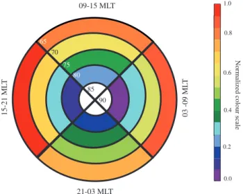
Table 3.Percentage of beam-swung vectors which are within a cone of 45◦around the merged angles, as a function of magnetic local time and magnetic latitude
Mag. 03:00–09:00 09:00–15:00 15:00–21:00 21:00–03:00
Latitude MLT MLT MLT MLT
60◦–65◦ No data No data No data No data
65◦–70◦ 69 67 75 59
70◦–75◦ 52 53 55 48
75◦–80◦ 33 37 32 35
80◦–85◦ 21 32 28 29
85◦–90◦ No data No data No data No data
the beam-swinging algorithm have a magnitude that is within 25% or 50 m/s (whichever is larger) of the magnitude esti-mated by the merging algorithm.
A study was performed to see whether the quality of the fit of the data was dependent upon time of day or the latitude at which the l-o-s vectors were observed. The data has been divided into four different time intervals, night (21:00–03:00 MLT), dawn (03:00–09:00 MLT), mid-day (09:00–15:00 MLT) and dusk (15:00–21:00 MLT) with six different latitude bins from 60◦to 90◦. Table 3 presents the percentage of beam-swung vectors which are within a cone of 45◦ around the merged angles as a function of lo-cal time and magnetic latitude. These results are also de-picted in Fig. 6. The colour bar is normalized, with red rep-resenting the region where there is the highest percentage of map-potential vectors within the same flow quadrant as the merged vectors and blue representing the region of lowest percentage of merged vectors within the same flow quad-rant as the merged vectors. The results show that the beam-swinging technique is most successful at predicting flow an-gles in the dusk and dawn sectors at low latitudes. Over-all, we found that the beam-swinging technique was most successful at predicting the angle of plasma flow at low lat-itude in the dusk sector, with 75% of the vectors being in the correct flow quadrant as compared with 48% of the data points when using all the available data (Table 1). The beam-swinging technique was least successful at estimating the correct flow quadrant at high latitude in the dawn sector; here only 21% of the angles were in the correct flow quadrant.
03 -09 ML
T
09-15 MLT
15-21 ML
T
21-03 MLT 65
70
75
80
85
90
Comparison between merged and beam-swung velocity direction as a function of latitude and local time.
1.0
0.8
0.6
0.4
0.2
0.0
Normalized colour scale
65
70
80
85
75
90
Table 4.Percentage of true map-potential vectors which are within a cone of 45◦around the merged angles, as a function of magnetic local time and magnetic latitude
Mag. 03:00–09:00 09:00–15:00 15:00–21:00 21:00–03:00
Latitude MLT MLT MLT MLT
60◦–65◦ No data No data No data No data
65◦–70◦ 80 84 83 70
70◦–75◦ 69 78 76 65
75◦–80◦ 51 60 53 56
80◦–85◦ 30 30 27 25
85◦–90◦ No data No data No data No data
0 90 180 270 360
Merge angle 0
90 180 270 360
Map potential angle
Normalised occurrence
Normalised occurrence Comparison between merged and
true map potential angles
Total number of data points 143401.
Fig. 7. Comparison between merged and “true” map-potential ve-locity directions. Also shown are the normalized occurrence distri-butions of the angles.
4.2 Comparison between merged and map-potential vec-tors
Having compared the merging technique with the beam-swinging technique, we proceed to compare the merging technique with the map-potential model. Figure 7 presents the scatter plot of the directions of the merged flow vectors with the “true” flow vectors, the normalized occurrence dis-tributions of the angles measured by both techniques are also shown. As before, angles are measured clockwise from geo-magnetic north and the 45◦line represents the idealized case where the map-potential technique perfectly reproduces the merged velocity estimates. As with the comparison between
the merged and beam-swung angles, there are two main clus-ters of points, one situated around 90◦, the other around 270◦. However, now there seems to be a general clustering of points around the 45◦ line for all angles, although there appears to be an offset of about 20◦between the velocity di-rections estimated by the map-potential and the merge tech-niques. The peak in the occurrence of data points in the dusk sector (14 871 data points) is more than twice as large as the peak in the occurrence of data points in the dawn sector (6135 data points).
We studied the cumulative percentage of map-potential de-rived velocity estimates within a given angular difference to the merged velocities. We found that 65% of the angles de-rived using the “fitted“ map-potential model lay inside a 45◦ cone around the merged velocity estimates; for the “true” vectors this value was 66% (Table 1). So there was no signifi-cant difference in the ability of the “fitted” and “true” vectors to correctly predict the correct flow quadrant. However, these values were a significant improvement on the beam-swinging technique, where only 48% of the un-filtered velocity esti-mates and 61% of the filtered velocity estiesti-mates were in the correct flow quadrant.
Each scan of data for the map-potential model has a χr2
value associated with it, which is a measurement of the good-ness of the fit. We filtered the “fitted” map-potential angles only including data which had an associatedχr2value of 1.5 or less. When comparing the filtered map-potential angles, with the merged velocity direction, only 64% of the filtered map-potential angles lay within a cone of 45◦ half-widths around the merged angles (Table 1). It would appear that theχr2value for each scan of the map-potential model is not significant when determining the algorithm’s ability to accu-rately predict the correct flow quadrant.
0 200 400 600 800 1000 Merge velocity
0 200 400 600 800 1000
Map potential velocity
0 200 400 600 800 1000
Merge velocity 0
200 400 600 800 1000
Map potential velocity
Comparison between merged and map_potential velocities
0.0 0.2 0.4 0.6 0.8 1.0
Normalised colour scale
Fig. 8. Comparison between merged and “true” map-potential ve-locity magnitude. The normalized occurrence distribution of data points is colour coded with red indicating regions of most data points and blue indicating region of fewest data points.
smaller than those estimated by the merging algorithm. A comparison was performed between the merged and the “fitted” and “true” map-potential velocity estimates, study-ing the cumulative percentage occurrence in the percentage difference in the velocity magnitudes estimated by the merg-ing algorithm as compared with the velocity magnitudes es-timated by the map-potential model. 41% of the flow vec-tors estimated by the map-potential model and the merging algorithm have magnitudes that are within 25% or 50 m/s (whichever is larger) of each other (Table 2), as compared with 49% of the “true” velocity vectors.
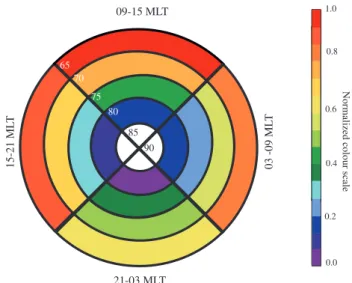
Finally, a study was performed to see whether the qual-ity of the fit of the data was dependent upon time of day or the latitude at which the l-o-s vectors were observed. Ta-ble 4 presents the percentage of map-potential vectors which are within a cone of 45◦ around the merged angles, calcu-lated separately for six longitude bins in four time separate time intervals, dawn (03:00–09:00 MLT), midday (09:00– 15:00 MLT), dusk (15:00–21:00 MLT) and night (21:00– 03:00 MLT). There were no vectors to compare between 60◦
and 65◦so the latitude runs from 65◦to 90◦. The results
pre-sented in Table 4 are also depicted in Fig. 9. The colour bar is normalized, with red representing the region where there is highest percentage of map-potential vectors within the same flow quadrant as the merged vectors, and blue rep-resenting the region of lowest percentage of merged vectors within the same flow quadrant as the merged vectors. The results show that the map-potential model is most successful at predicting flow angles in the dusk and day sectors at low latitudes. Overall, we found that the map-potential technique was most successful at predicting the angle of plasma flow at low latitude in the day sector, with 84% of the vectors being
03 -09 ML
T
09-15 MLT
15-21 ML
T
21-03 MLT 65
70
75
80
85 90
Comparison between merged and true map-potential velocity direction as a function of latitude and local time.
1.0
0.8
0.6
0.4
0.2
0.0
Normalized colour scale
65 70
75 80
85 90
Fig. 9. Comparison between merged and “true” map-potential ve-locity directions, as a function of magnetic latitude and magnetic local time. The diagram is colour coded with red indicating the re-gion where there is the highest percentage of beam-swung vectors within the same flow quadrant as the merged vectors, and blue rep-resenting the region where there is the lowest.
in the correct flow quadrant, as compared with 66% of the data points when using all the available data (Table 1). 50% of the “true” map-potential velocities estimated at this time and latitude had a magnitude within 25% or 50 m/s of the merged velocity magnitudes (Table 2). The technique was least successful at predicting the correct flow angle at high latitudes in the night sector; here only 25% of the vectors were in the correct flow quadrant.
5 Discussion
Figures 4 and 7 present scatter plots of the direction of the merged flow vectors with the beam-swung vectors and the “true” map-potential flow vectors, respectively. Both tech-niques result in two main clusters of points, one situated at 90◦, due to eastward flow measured by the radar in the dawn convection cell, the other cluster is around 270◦, due to west-ward flow in the dusk convection cell. However, when com-paring the merged and the “true” map-potential vectors there is also a general clustering of points around the 45◦ line, not present for the beam-swung vectors. This shows that the map-potential algorithm is capable of accurately deter-mining non L-shell aligned convection flow which is poorly estimated by the beam-swinging technique as it makes in-correct assumptions about the flow patterns in these regions. This demonstrates that the map-potential technique, with its incorporated statistical model, makes much more realistic assumptions about the flow pattern than the simple beam-swinging technique.
The flow angles estimated by both the beam-swinging and the map-potential techniques are offset by about 20◦to those calculated by the merging technique, representing an aver-age southward tilt of the map-potential and beam-swung de-rived velocities as compared with the merged velocities in the dawn sector and, conversely, an average northward tilt in the dusk convection cell. At present we can offer no explanation for this offset. All three algorithms appear to preferentially detect flow in the dusk convection cell. However, whereas the map-potential model observed approximately 140% more data points in the dusk sector than the dawn sector, this was reduced to 100% for the merging algorithm and to only 40% for the beam-swinging algorithm.
We compared the cumulative percentage of the velocity di-rections derived by the beam-swinging and the map-potential techniques within a given angular difference to the merged velocity direction (see Table 1). 48% of the data points cal-culated by the beam-swinging technique were in the correct flow quadrant, as compared to 65% of the data calculated by the “fitted” map-potential model and 66% of the data points calculated by the “true” map-potential method. So al-though there was no significant difference in the ability of the “true” and “fitted” map-potential vectors to correctly pdict the correct flow quadrant, the map-potential model re-sulted in a significant improvement in accurately predicting the flow angle of ionospheric vectors as compared with the beam-swinging technique.
We have attempted to utilise several quality flags in or-der to remove less accurate data but without success. When comparing the flow direction of the vectors calculated by the merged and swung methods, we discarded all beam-swung velocities with a rms error of more than 150 m/s. Of the remaining vectors, 61% of the data points accurately pre-dicted the correct flow quadrant as compared to 48% of the data points when all the flow vectors where included. So, fil-tering the data using the rms error, results in a 13% improve-ment in the ability of the data to correctly predict the flow angle of the ionospheric flow. However the proportion of filtered beam-swung vectors that are within the correct flow
quadrant is still less than those of the “true” map-potential vectors. When comparing the map-potential velocity esti-mates, we removed all the data points which had aχr2greater than 1.5 associated with them. However, there was no signif-icant difference in the ability of the vectors to predict the cor-rect flow quadrant, suggesting that theχr2parameter is not a particularly accurate quality-of-fit parameter but, rather, that the accuracy of the assumptions underlying the technique de-termines the fit quality.
Figures 5 and 8 present comparisons of the magnitude of the flow vectors calculated using the merged/beam-swung and the merged/map-potential techniques, respectively. The velocities estimated by all three techniques are mainly be-tween 50 and 300 m/s. The velocity magnitudes estimated by the beam-swinging algorithm appear to be of the same mag-nitude as the velocity magmag-nitudes estimated by the merging algorithm. Figure 8 would suggest that “true” velocities es-timated by the map-potential model are slightly smaller than those estimated by the merging algorithm. This may be due to the spatial and temporal filtering performed on the map-potential vectors.
Table 2 presents a comparison of the magnitude of the beam-swung and “true” map-potential vectors with the mag-nitude of the merged vectors. 31% of the beam-swung vec-tors had a magnitude that was within 25% of the merged velocity magnitude as compared with 41% of the “fitted” and 49% of the “true” map-potential flow vectors. So “true” map-potential flow vectors are significantly more successful at predicting the magnitude of the plasma flow than the “fit-ted” map-potential vectors or the beam-swung vectors.
the beam-swinging technique. Both the map-potential and the beam-swinging techniques perform poorly in the night sector, showing that the unstructured flow observed at such high latitude is difficult to reproduce by any technique which makes assumptions about the direction of plasma flow; no matter whether these assumptions involve predicting the flow to be zonal or are based on using a statistical model when de-termining the plasma flow pattern.
In this paper we have used the 1998 version of the map-potential technique. Over the past few years several changes have been made to the map-potential technique, as described in Shepherd and Ruohoniemi (2000). We have compared vectors derived by the map-potential and merging tech-niques. These two techniques are very different and perfect agreement between the vectors derived by them is not ex-pected due to HF noise and misidentified ground scatter con-taminating the l-o-s velocity data. The merging technique aims to derive the best local solution while the map-potential technique derives global solutions. Thus the merging tech-nique can show sources and sinks in the flow; however this behaviour is not consistent with a potential solution. Finally, in this paper, the merging technique is assumed to be the most accurate method of deriving flow vectors from l-o-s veloci-ties as the technique does not depend on a statistical model or make any assumptions about the direction of the plasma flow. However, the merging technique is still subject to the possible measurement errors outlined above and there is also the possibility of error if the angle separating the two merged l-o-s velocity measurements is small.
The map-potential vectors were only obtained using l-o-s flow vectors from one of the Northern hemisphere Super-DARN radar pairs. In reality the model is best run using all the available l-o-s velocities from all six pairs of North-ern hemisphere SuperDARN radars with the model being run on a case-by-case basis where parameters such as the order of fit and low-latitude boundary can be adjusted for the in-dividual measurements. We would assume that, if the map-potential model used more l-o-s velocities when calculating the convection flow vectors, the resulting vectors would be even more accurate. However, the authors are aware that this study is only using the map-potential model in regions where predicted flow vectors are most dependent on observed l-o-s velocity as these are the regions where it is possible to obtain merged flow vectors. Had we been able to perform a similar study of the map-potential vectors obtained further from the radar fields-of-view (and thus more dependent on the statis-tical model) the results might have been different.
Yeoman et al. (1992) assessed the beam-swinging tech-nique as used to study E-region irregularity drift patterns with data from the SABRE radars. The L-shell “fitted” veloci-ties were calculated under two different sets of constraints: a “loosely constrained” fit, where the radar data were required to fill at least five of the eight SABRE beams and the rms error of the least square fit of the L-shell was required to be less than 75 m/s. In addition a set of “tightly constrained” fits was calculated, in which at least seven out of the eight SABRE beams were filled with backscatter and a rms error
of less than 50 m/s was required. A third set of tightly strained fits were calculated which included the extra con-straint than no l-o-s velocity anywhere in the field-of-view of either of the SABRE radars exceeded 500 m/s. The study concentrated on the direction of the velocity vectors, as ve-locity magnitude of both the merged and the beam-swung vectors were constrained due to sound speed limiting. 74% of the “loosely constrained” beam-swung angles lie inside a cone of 45◦half-width around the SABRE merged velocities with 82% of the tightly constrained l-o-s velocities and 84% of the filtered l-o-s velocity lying within a cone of 45◦ half-width. This compares with 48% of the SuperDARN beam-swung vectors and 84% of the “fitted” map-potential vec-tors observed in the dawn sector within 65◦and 70◦latitude. Thus the SABRE filtered beam-swung vectors are as effec-tive at mapping the direction of ionospheric flow as the “true” map-potential vectors at low latitudes in the dawn sector. We believe that SuperDARN beam-swung vectors are less suc-cessful at mapping the direction of ionospheric flow than the SABRE vectors because SABRE was a VHF radar observing mainly low-latitude return flow in the E-region, while Su-perDARN is a HF radar observing at higher latitudes where HF radar suffers from problems of HF noise and misidenti-fied ground scatter. Also beam-swinging assumes a homoge-neous flow along the L-shells; as SABRE has a much smaller field-of-view than the SuperDARN radars there will be less variation in the flow across it.
6 Summary
This study has entailed a comparison of the merged, map-potential (1998 version), L-shell “fitting” and beam-swinging techniques when predicting the ionospheric flow vectors using l-o-s velocity data from the SuperDARN HF radars. For the first time, quantitative information has been provided about the validity of the map-potential technique, which is becoming the main source of real-time informa-tion about global convecinforma-tion. We can conclude that the map-potential model is significantly more successful than the beam-swinging technique at estimating both the magnitude and the direction of the convection flow vectors, even when the beam-swung vectors are filtered using an rms error anal-ysis. The quality of the fit is dependent on location and time of day, with the “fitted” and “true” map-potential vectors pre-dicting the direction of the flow most successfully at low lat-itudes in the day sector. There is no significant difference in the ability of the “true” or “fitted” map-potential vectors to recreate the direction of convective flow vectors but the “true” map-potential vector re-creates the magnitude of the convective flow vectors more successfully than the “fitted” vectors.
Acknowledgements. CUTLASS is supported by the
The authors wish to thank C. Senior and J.-C. Cerisier for develop-ing the SuperDARN mergdevelop-ing software.
The Editor in Chief thanks J. Holt for his help in evaluating this paper.
References
Andr´e, D., McNamara, A. G., Wallis, D. D., McIntosh, B. A., Hughes, T. J., Sofko, G. J., Koehler, J. A., McDiarmid, D. R., Prikryl, P., and Watermann, J.: Diurnal radio aurora variations at 50 MHz measured by the Bistatic Auroral Radar System radars, J. Geophys. Res., 8651–8661, 1988.
Bristow, W. A., Ruohoniemi, J. M., and Greenwald, R. A.: Super Dual Auroral Radar Network observations of convection during a period of small-magnitude northward IMF, J. Geophys. Res., 103, 4051–4061, 1998.
Davies, J. A., Lester, M., Milan, S. E., and Yeoman, T. K.: A com-parison of F-region ion velocity observations from the EISCAT Svalbard and VHF radars with irregularity drift velocity mea-surements from the CUTLASS Finland HF radar, Ann. Geophys-icae, 18, 589–594, 2000.
Davies, J. A., Lester, M., Milan, S. E., and Yeoman, T. K.: A com-parison of velocity measurements from the CUTLASS Finland radar and EISCAT UHF system, Ann. Geophysicae, 17, 892– 902, 1999.
Fejer, B. G. and Kelley, M. C.: Ionospheric irregularities, Rev. Geo-phys., 18, 401–454, 1980.
Freeman, M. P., Ruohoniemi, J. M., and Greenwald, R. A.: The de-termination of time-stationary two-dimensional convection pat-terns with single-stations radars, J. Geophys. Res, 96, 15 735– 15 749, 1991.
Greenwald, R. A., Weiss, W., Nielsen, E., and Thomson, N. R.: STARE: A new radar auroral backscatter experiment in northern Scandinavia, Radio Sci., 13, 1021–1039, 1978.
Greenwald, R. A., et al.: DARN/SuperDARN: A global view of high-latitude convection, Space Sci. Rev., 71, 761–796, 1995. Hanuise, C., Senior, C., Cerisier, J.-C., Villain, J.-P., Greenwald, R.
A., Ruohoniemi, J. M., and Baker, K. B.: Instantaneous mapping of high-latitude convection with coherent HF radars, J. Geophys. Res, 98, 17 387–17 400, 1993.
Jackson, J. D.: Classical Electrodynamics, John Wiley, New York, 1962.
Kofman, W. and Nielsen, E.: STARE and EISCAT measurements: Evidence for the limitation of STARE Doppler velocity observa-tions by the ion acoustic velocity, J. Geophys. Res., 95, 19 131– 19 135, 1990.
Lepping, R. P., et al.: The WIND magnetic field investigation, Space. Sci. Rev., 71, 207–229, 1995.
Lester, M., de la Beujardi`ere, O., Foster, J. C., Freeman, M. P., L¨uhr, H., Ruohoniemi, J. M., and Swider, W.: The response
of the large scale ionospheric convection pattern to changes in the IMF and substorms: Results from the SUNDIAL 1987 cam-paign, Ann. Geophysicae, 11, 556–571, 1993
Nielsen, E. and Schlegel, K.: A first comparison of STARE and EISCAT electron drift velocity measurements, J. Geophys. Res., 88, 5745–5750, 1983.
Nielsen, E. and Schlegel, K.: Coherent radar Doppler measure-ments and their relationship to the ionospheric electron drift ve-locity, J. Geophys. Res., 90. 3498–3504, 1985.
Nielsen, E., Guttler, W., Thomas, E. C., Steward, C. P., Jones, T. B., and Hedburg, A.: SABRE – A new radar auroral backscatter experiment, Nature, 304, 712–714, 1983.
Richmond, A. D and Kamide, Y.: Mapping electrodynamic fea-tures of the high-latitude ionosphere from localized observations: Technique, J. Geophys. Res., 93, 5741–5759, 1988.
Robinson, T. R.: Towards a self-consistent non-linear theory of radar auroral backscatter, J. Atmos. Terr. Phys., 48, 417–422, 1986.
Ruohoniemi, J. M., Greenwald, R. A., Baker, K. B., Vil-lain, J.-P., and McCready, M. A.: Drift motions of small-scaleirregularitiesin the high-latitude F-region: An experimen-tal comparison with plasma drift motions, J. Geophys. Res., 92, 4553–4564, 1987.
Ruohoniemi, J. M., Greenwald, R. A., Baker, K. B., Baker, K. B., Villain, J.-P., Hanuise, C., and Kelley, J.: Mapping high-latitude plasma convection with coherent HF radars, J. Geophys. Res., 94, 13 463–13 477, 1989.
Ruohoniemi, J. M. and Greenwald, R. A.: Statistical patterns of high-latitude convection obtained from Goose Bay HF radar ob-servations, J. Geophys. Res., 101, 21 743–21 763, 1996. Ruohoniemi, J. M. and Baker, K. B.: Large-scale imaging of
high-latitude convection with Super Dual Auroral Radar Network HF radar observations, J. Geophys. Res., 103, 20 797–20 811, 1998. Shepherd, S. G. and Ruohoniemi, J. M.: Electrostatic potential pat-terns in the high-latitude ionosphere constrained by SuperDARN measurements, J. Geophys. Res., 105, 23 005–23 014, 2000. Villain, J.-P., Caudal, G., and Hanuise, C.: A SAFARI-EISCAT
comparison between the velocity of F-region small-scale irregu-larities and the ion drift, J. Geophys. Res., 90, 8433–8443, 1985. Villain, J.P., Greenwald, R. A., Baker, K. B., and Ruohoniemi, J. M.: HF radar observations of E-region plasma irregularities produced by oblique plasma streaming, J. Geophys. Res, 92, 12 327–12 342, 1987.
Weimer, D. R.: Models of high-latitude electric potentials derived with a least error fit of spherical harmonic coefficients, J. Geo-phys. Res., 100, 19 595–19 607, 1995.