Rev. Adm. (São Paulo) vol.52 número4

(1)

Availableonlineatwww.sciencedirect.com

Revista

de

Administração

http://rausp.usp.br/ RevistadeAdministração52(2017)403–418

Finance

and

Accounting

Volatility

persistence

and

inventory

effect

in

grain

futures

markets:

evidence

from

a

recursive

model

Persistência

de

volatilidade

e

efeito

de

inventário

nos

mercados

de

futuros

de

grãos:

evidência

de

um

modelo

recursivo

Persistencia

de

volatilidad

y

efecto

de

inventario

en

los

mercados

de

futuros

de

granos:

evidencia

de

un

modelo

recursivo

Rodrigo

Lanna

Franco

da

Silveira

a,∗

,

Leandro

dos

Santos

Maciel

b

,

Fabio

L. Mattos

c

,

Rosangela

Ballini

a

a_University_of_Campinas,_Campinas,_SP,_Brazil b_Federal_University_of_São_Paulo,_São_Paulo,_SP,_Brazil

c_University_of_Nebraska,_Lincoln,_NE,_United_States

Received10May2016;accepted29May2017

Availableonline8September2017

ScientificEditor:DanielReedBergmann

Abstract

Thepurposeofthispaperistoinvestigatethevolatilitypersistenceandtheinventoryeffectingrainfuturesmarketsduringtheperiodof1959–2014. Theinnovativenatureofthisstudyliesintheevaluationofrollingestimates,usingarecursiveunivariateTARCH(1,1)-in-meanvolatilitymodel. Thedailyevolutionofvolatilitypersistenceandtheinventoryeffectoncornandsoybeanfuturescontractsisanalyzedusingarollingwindowof 1008observationsoverfouryears.Ingeneral,theresultssuggestthattheconditionalvolatilityinbothmarketsishighlypersistent.Thereisalso evidenceofinventory,time-to-maturity,andseasonalityeffectsonthevolatilitydynamicsofcornandsoybeans.Inaddition,thefindingspointto alowershort-runvolatilitypersistenceinrecentyears,whichcausedaslightdecreaseinlong-runvolatilitypersistenceandthehalf-lifeperiodin bothmarkets.

©2017DepartamentodeAdministração,FaculdadedeEconomia,AdministraçãoeContabilidadedaUniversidadedeSãoPaulo–FEA/USP. PublishedbyElsevierEditoraLtda.ThisisanopenaccessarticleundertheCCBYlicense(http://creativecommons.org/licenses/by/4.0/).

Keywords:Pricevolatility;Volatilitypersistence;Inventoryeffect;Grainfuturesmarkets

Resumo

Nesteartigo,osautoresprocuraraminvestigarapersistênciadavolatilidadeeinventoryeffectnosmercadosfuturosdegrãosnoperíodoentre 1959e2014.AinovaçãodoestudoconsistiunaaplicaçãodeummodelodevolatilidaderecursivoTARCH(1,1)comrolagemdasestimativasa partirdeumajaneladetempodequatroanos.Osresultadosapontaramparaumaaltapersistênciadavolatilidadecondicionalnosmercadosde milhoesoja.Alémdisso,observou-seapresençadosefeitossazonalidade,inventoryetime-to-maturitynadinâmicadevolatilidadedospreçosde

∗_{Corresponding}_author_at:_{Unicamp/Instituto}_de_Economia,_CP_6135,_sala_68,_CEP_13085-970_Campinas,_SP,_Brazil.

E-mail:[email protected](R.L.Silveira).

PeerReviewundertheresponsibilityofDepartamentodeAdministrac¸ão,FaculdadedeEconomia,Administrac¸ãoeContabilidadedaUniversidadedeSão

Paulo–FEA/USP.

https://doi.org/10.1016/j.rausp.2017.08.003

(2)

ambosmercados.Verificou-seaindaumaquedanapersistênciadecurto-prazonoperíodorecente,oquelevouaumadiminuic¸ãodapersistência delongo-prazoedameia-vidanosmercadosemestudo.

©2017DepartamentodeAdministração,FaculdadedeEconomia,AdministraçãoeContabilidadedaUniversidadedeSãoPaulo–FEA/USP. PublicadoporElsevierEditoraLtda.Este éumartigoOpenAccesssobumalicençaCCBY(http://creativecommons.org/licenses/by/4.0/).

Resumen

Elobjetivoenesteestudioesinvestigarlapersistenciadelavolatilidadyelefectodeinventarioenlosmercadosdefuturosdegranosenelperíodo de1959a2014.LainnovacióndeltrabajoconsisteenlaaplicacióndeunmodelodevolatilidadrecursivoTARCH(1,1)porestimación,enun períododecuatroa˜nos.Losresultadosindicanunaaltapersistenciadelavolatilidadcondicionalenelmercadodemaízysoja.Además,hay evidenciadeefectosdeinventario,tiempohastalaexpiraciónyestacionalidadenladinámicadelavolatilidaddelospreciosdeambosmercados. Tambiénsehaverificadounabajapersistenciadelavolatilidadacortoplazoenlosúltimosa˜nos,loquehacausadounacaídadelapersistencia delavolatilidadalargoplazo.

©2017DepartamentodeAdministração,FaculdadedeEconomia,AdministraçãoeContabilidadedaUniversidadedeSãoPaulo–FEA/USP. PublicadoporElsevierEditoraLtda.Esteesunart´ıculoOpenAccessbajolalicenciaCCBY(http://creativecommons.org/licenses/by/4.0/).

Palavras-chave: Volatilidade;Persistênciadavolatilidade;Inventoryeffect;Mercadofuturodegrãos

Palabrasclave: Volatilidad;Persistenciadelavolatilidad;Efectodeinventario;Mercadofuturodegranos

Introduction

Theanalysisofpricevolatilityinagriculturalmarketsplays an importantrole inthe decision-makingprocess.Price vari-ation influences decision-making in the case of production, marketing,andriskmanagementinagriculture.Highprice fluc-tuations affectproducer’s profitability, even when production isveryefficient.Theseeventsalsoaffectpolicymakers, espe-ciallyindevelopingcountries,sincepriceandvolatilitylevels impactfood security,balanceof trade,inflation rate,tax rev-enue,employment,GDP,andbusinesscycles.Additionally,in financial markets, price oscillations are relevant in portfolio allocationandderivativespricing (Ghoshray,2013;Naylor &

Falcon,2010).

During the 2000s, many agricultural commodities experi-enceda sharp andrapidriseinprice.While overthe second half of the 1970s and 1990s, in particular in the 1980s, theinflation-adjustedWorldBankagricultureindexdecreased 58%, a sharp price spike of around 40% occurred during 2005–2008.Agriculturalcommodities,suchascorn,wheat,and soybeansexhibitedapriceincreaseofmorethan60%overthis period.

Previousstudieshaveinvestigatedthefactorsunderlyingthis scenario.Severalexplanationsweregiven,suchasanincreasing demandforbiofuelfromgrainsandoilseeds,risingoilprices, agrowthindemandforcommodities(especiallyintheBRICS countries– Brazil,Russia,India,China, andSouthAfrica),a reduction insubsidiesforEuropean farmers, adverseweather conditions,lowinventorylevels,depreciationoftheU.S. dol-lar,andanincreaseinspeculativetransactionsincommodities futuresmarkets(Gilbert,2010;Headey&Fan,2008;Sumner,

2009).

Recentstudieshaveexploredthepricefluctuationsof agri-culturalcommoditiesinordertoverifytheexistenceofvolatility breaksinthefirstdecadeofthe2000s(Calvo-Gonzalez,Shankar,

& Trezzi, 2010; Gilbert & Morgan, 2010; Huchet-Bourdon,

2011;Sumner,2009;Vivian&Wohar,2012).Ingeneral,noclear

evidencewasfoundtosupporttheideathattherecentprice vari-ability wasunparalleled.However,two importantissueshave received relatively little attention, namely the persistence of pricevolatilityandtheleverageeffect(alsoknownasthe “inven-tory effect”,inthecaseofcommodities).Even ifagricultural markets are notexperiencing unprecedentedlevels of volatil-ity,itisstill crucialtounderstandhowlongittakesvolatility to revert toits previous level after a shock.In addition, it is importanttoverifytheasymmetryinthevolatilityprocess.In agriculturalmarkets,incontrasttoequitymarkets,positiveprice shocks(“badnews”)tendtohavealargerimpactonconditional variance thannegativepriceshocks(“goodnews”).This phe-nomenonisknownastheinventoryeffect(Carpantier,2010)and canbeexplainedbythestoragemodel.1 Volatilitypersistence andinventoryeffectsaffectagriculturalproducers’,buyers’,and traders’exposuretorisk,thusinfluencingriskmanagement oper-ations(Carpantier&Samkharadze,2013).Morebroadly,these issuesarerelevantforcountriesthatrelyheavilyonexportsand importsofagriculturalcommodities,aswellastoevaluate infla-tionary processes and formulate price stabilization programs

(Ghoshray,2013;Vivian&Wohar,2012).

This paper explores the volatility persistence and inven-toryeffectongrainfuturesmarketsoverthelastdecades.The research uses daily futures prices of two commodities (corn and soybeans). A recursive univariate TARCH(1,1)-in-mean volatility model is applied tocompute the daily evolution of the volatility persistence andthe inventory effectin terms of rolling estimates. Thus, the study investigates whether there havebeen changesinthesetwo measuresovertimeandtheir implicationsfor agriculturalmarkets.Thestudy alsoanalyzes

1_A_decrease_in_the_commodity_inventory_levels,_originating_from_a_scenario

ofsupplyshortagesand/ordemandexpansionrelatedtothiscommodity,tend

tocauseanincreaseinitsprice.Theinventoryeffectconsidersthatthereaction

tocommodityreturnsishigherforpositivepriceshocksthantonegativeshocks

(3)

R.L.F.Silveiraetal./RevistadeAdministração52(2017)403–418 405

otherdeterminantsofagriculturalcommodityvolatilityinmodel specification,suchasseasonalityandtime-to-maturity.

Previousstudies

Several empirical studies have employed different approaches to investigate the volatility dynamics in agri-cultural markets. These studies can be categorized into five maingroups.Thefirst oneevaluatedandcomparedpriceand volatility evolution between agricultural commodities and manufacturedgoods.Prebisch(1950)andSinger(1950)began this analysis and, more recently, other research has focused onprice volatility, such as Jacks, O’Rourke, andWilliamson

(2011),Arezki,Hadri,Loungani,andRao(2014)andArezki,

Lederman, and Zhao (2014). The second group of studies

analyzedtheimpactof commoditypricevolatilityonincome and welfare in developing countries (Bellemare, Barrett, &

Just,2013;Blattman,Hwang,&Williamson,2007;Naylor &

Falcon,2010;Rapsomanikis&Sarris,2008).

Athirdgroupofstudiescomparedcommodityprice volatil-itybetweenthefirstdecadeofthe21stcenturyandtheprevious decadesofthe20thcentury.Ingeneral,theresultsshowedthat pricevariabilityover2006–2010wasnothigherthanthe volatil-ityobservedin1970(Gilbert&Morgan,2010;Huchet-Bourdon,

2011).Calvo-Gonzalezetal.(2010)highlightedthreeperiodsof

relevantvolatilitybreaks–duringthetwoworldwarsandduring thetimewhentheBrettonWoodssystemcollapsed.Despitethe factthatthecommodityvolatilitylevelduringthe2000swasnot unparalleled,relevantspikeswereobservedfrom2005to2008. Consequently,anumberofworkshaveevaluatedthecausesof therisingvolatility,enumeratingfactorssuchasthefast expan-sionof biofuel production, increasingoil prices,depreciation of theU.S. dollar,lowerlevel of inventoriesandthe “finan-cialization”ofcommoditymarkets(Arezki,Loungani,Ploeg,&

Venables,2014;Balcombe,2009;Beckmann&Czudaj,2014;

Du,Yu,&Hayes,2011;Mensi,Beljid,Boubaker,&Managi,

2013;Nazlioglu,Erdem,&Soytas,2013;Power&Robinson,

2013;Serra,2011;Wright,2011).

Inaddition,afourthgroupofstudiesanalyzedthe determi-nants of agricultural commodity price volatility. Seasonality, time-to-maturity,2 inventory level, volatility persistence, day-of-the-week,futuresmarkettradingvolume,speculativeactivity, loanratelevel,pricelevel,amongothers,wereanalyzedinorder toverifytheirinfluenceonagriculturalcommodityprice fluc-tuation. Table1 present asummaryof thisliterature andthe followingparagraphsaddresstherecentstudies.

A numberof works have identified seasonality and time-to-maturityasimportantdeterminantsofagriculturalvolatility.

2 _The_{time-to-maturity}_effect_is_also_known_as_the_Samuelson_effect._According

totheSamuelsonhypothesis,futurespricevolatilitytendstoincreaseasthe

futurescontractmaturitydateapproaches.Whenafuturescontractapproachesits

expiration,“thepriceofanexpiringcontractmustvirtuallyequaltheprevailing

spotprice,nearercontractstendtorespondstronglytonewinformationsothat

thepriceofanexpiringfuturescontractwillconvergetothespotprice”(Milonas,

1986,p.445).

KalevandDuong(2008)andDuongandKalev(2008),using

intradaydata,verifiedthematurityeffectinagriculturalfutures markets.Inaddition,KaraliandThurman(2010)identifiedthe presenceof seasonalityandmaturityeffectsincorn,soybean, wheat,andoatsmarketsbetween1986and2007.Karalietal.

(2010) showed that the volatility of corn, soybean, and oats

futurespriceswasaffectedbytime-to-maturity,inventories,and progressofthecrop(with,ingeneral,ahigherpricefluctuation beforethebeginningoftheharvest).VermaandKumar(2010)

and Gupta and Rajib (2012) also contributed to this debate,

examining the time-to-maturity effect in Indian futures mar-kets.On onehand,Verma andKumar (2010)foundevidence of amaturityeffectinwheatandpepperfuturesmarkets. On theotherhand,GuptaandRajib(2012),focusing theanalysis oneightcommoditiesfuturesmarkets(includingwheatfutures contract),indicatedthatthefuturescontracttradingvolumehas ahighereffectonthevolatilitythantime-to-maturity.He,Yang,

Xie,andHan(2014)confirmedtheimportanceofthevolume

effectonpricevolatility, bystudying sixcommoditiesfutures marketsinChina.

Many studies have also indicated the inventory effect as a relevant factor that influences agricultural price variability.

Carpantier (2010) analyzed 15 commodity price series over

1994–2009 and found that there was an inventory effect in coffee, soybean, and wheat markets. A similar analysis was carried out by Carpantier and Dufays (2012), analyzing 16 commoditiesfrom1994to2011.Alloftheestimated asymmet-riccoefficientsforagriculturalmarkets(corn,cotton,soybean, sugar, wheat,andcoffee)werenegative,however,onlyinthe casesofsugarandcoffeeweretheparametersstatistically differ-entfromzero.StiglerandPrakash(2011)verifiedtwodistinct levels of unconditional volatilityin the wheatmarket, where one regime oscillated between 20 and 36 times higher than theotherregime.Theauthorsshowedthatthehighervolatility regime emergedwhen theUnitedStatesDepartmentof Agri-culture(USDA)forecastspointedtoalowinventorylevel(bad newsonstocks-to-disappearance).Conversely,whentheUSDA inventoryforecastsindicatednomarkettightness(positivenews onstocks-to-disappearance),therewasnoapparentrelationship betweenwheatpricesandinventorylevel.

Finally, thevolatilitypersistence of agricultural commodi-tieswasevaluatedbyafifthgroupofstudies.Balcombe(2009)

investigatedthefactorsthatdrovethevolatilityof19agricultural commoditiesoverthelastdecades.Henotonlyfoundevidence of ahighvolatilitypersistenceinallpriceseriesbutalsothat oilvolatility,inventory levels,andyieldsinfluenceprice vari-ability.VivianandWohar(2012)indicated,ingeneral,ahigh volatilitypersistenceconsidering28commodities(grains, ani-mals,metals,andenergy)overtheyears1985–2010.Ghoshray

(2013)alsoexaminedthevolatilitypersistenceof24commodity

pricesseriesduringthe1900–2008period.Theresultssuggested thatthevolatilitypersistencevariessignificantlyovertimeand between different products. Using a spline-GARCH model,

Karali andPower (2013)foundthat the volatilitypersistence

(4)

R.

L.

F.

Silveir

a

et

al.

/

Re

vista

de

Administr

ação

52

(2017)

403–418

Table1

Summaryofliteraturereviewsregardingthedeterminantsofagriculturalcommodityvolatility.

Reference Method Variables Period(data

frequency)

Seasonality effect

Time-to-maturity effect

Inventory effect

Trade effect

Speculative

activityeffect

Loanrate

effect

Pricelevel

effect

Volatility persistence

effect

Y N NS Y N NS Y N NS Y N NS Y N NS Y N NS Y N NS Y N NS

Rutledge (1976)

Statisticaltests Silver,cocoa,

wheatand

soybeanoil

1969–1971 (daily)

X X X X X X X X

Anderson (1985)

Testsfor

equalityof

variancesand

regression analysis

9commodity

futuresprices

(8agricultural)

1966–1980 (daily)

X X X X X X X X

Milonas (1986)

Testsfor

equalityof

variancesand

regression analysis

11futures

prices(5

agricultural)

1972–1983 (daily)

X X X X X X X X

Kenyon, Kling, Jordan, Seale,and McCabe (1987)

Regression analysis

Corn,soybean,

wheat,live

cattleandlive

hogfutures

prices

1974–1983 (daily)

X X X X X X X X

Glauberand Heifner’s (1986)

Regression analysis

Soybean

futuresprice

1961–1984 (daily)

X X X X X X X X

Streeterand Tomek (1992)

Regression analysis

Soybean

futuresprices

1976–1986 (daily)

X X X X X X X X

Khouryand Yourougou (1993)

Regression analysis

Canola,rye,

feedbarley,

feedwheat,

flaxseed,and

oatsfutures

prices

1980–1989 (daily)

X X X X X X X X

Bessembinder andSeguin (1993)

Regression analysis

8futures

prices(2

agricultural)

1982–1990 (daily)

X X X X X X X X

Yangand Brorsen (1993)

GARCHand

deterministic chaos processes

11futures

prices(7

agricultural)

1979–88 (daily)

(5)

R.

L.

F.

Silveir

a

et

al.

/

Re

vista

de

Administr

ação

52

(2017)

403–418

407

Table1

(Continued)

frequency)

Seasonality effect

Inventory effect

Trade effect

Speculative

activityeffect

Loanrate

effect

Pricelevel

effect

Hennessyand Wahl(1996)

Contingent claims methodology

Corn,

soybeansand

wheat

1985–94 (monthly)

X X X X X X X X

Kocagiland Shachmurove (1998)

Time-series analysis

16futures

prices(6

agricultural)

1980–1995 (daily)

X X X X X X X X

Malliarisand Urrutia (1998)

Time-series analysis

Corn,wheat,

oats,soybean,

soybeanmeal,

andsoybean

oil

1981–1995 (daily)

X X X X X X X X

Hudsonand Coble (1999)

GARCH models

Cottonfutures

prices (monthly)

1982–97 (monthly)

X X X X X X X

Goodwinand Schnepf (2000)

GARCHand

VARmodels

Cornand

wheatfutures

prices

1986–1997 (weekly)

X X X X X X X X

Allenand Cruick-shank (2000)

Regression

analysisand

ARCHmodels

12commodity

futuresprices

(9agricultural)

1979–1998 (daily)

X X X X X X X X

Chatrath, Adrangi, andDhanda (2002)

Chaostests Corn,

soybeans,

wheatand

cottonfutures

prices

1968–1995 (daily)

X X X X X X X X

Yang,Balyeat, and Leatham (2005)

Granger

causalitytests

Corn, soybeans,

wheat,sugar,

coffee,live

cattleand

cottonfutures

prices

1992–2001 X X X X X X X X

Smith(2005) Partially overlapping

timeseries

model

Cornfutures

prices

1991–2000 (daily)

(6)

R.

L.

F.

Silveir

a

et

al.

/

Re

vista

de

Administr

ação

52

(2017)

403–418

Table1

(Continued)

frequency)

Seasonality effect

Inventory effect

Trade effect

Speculative

activityeffect

Loanrate

effect

Pricelevel

effect

Daal,Farhat, andWei (2006)

Regression analysis

61futures

contracts(23

agricultural)

1960–2000 (daily)

X X X X X X X X

Duongand Kalev (2008)

Non-parametricand

regression-basedtests;

GARCH model

Tick-by-tick

andbid-ask

quoteprices

for20futures

markets(10

agricultural)

1996–2003 (intraday)

X X X X X X X X

Kalevand Duong (2008)

Nonparametric

testand

regression analysis

14futures

prices(10

agricultural)

1996–2003 (intraday)

X X X X X X X X X

Balcombe (2009)

Decomposition

andpanel

approaches

19agricultural

spotprices

Varies

(monthly–annual)

X X X X X X X X

Karaliand Thurman (2010)

GLS estimation

Corn,soybean,

wheat,and

oatsfutures

price

1986–2007 (daily)

X X X X X X X X

Karali, Dorfman, and Thurman (2010)

Smoothed Bayesian estimator

Corn,

soybeans,and

oatsfutures

prices

Varied(daily) X X X X X X X X

Carpantier (2010)

GJR-GARCH

andEGARCH

models

15commodity

spotprices(5

agricultural)

1994–2009 (daily)

X X X X X X X X

Vermaand Kumar (2010)

Regression analysis

Wheatand

pepperfutures

prices

2004–2007 (daily)

X X X X X X X X

Stiglerand Prakash (2011)

Markov regime-switching GARCH

16commodity

spotprices

1985–2009 (daily)

X X X X X X X X

Carpantierand Dufays (2012)

GJR-GARCH model

16commodity

spotprices(7

agricultural)

1994–2011 (weekly)

(7)

R.

L.

F.

Silveir

a

et

al.

/

Re

vista

de

Administr

ação

52

(2017)

403–418

409

Table1(Continued)

frequency)

Seasonality effect

Inventory effect

Trade effect

Speculative

activityeffect

Loanrate

effect

Pricelevel

effect

Vivianand Wohar (2012)

Iterative cumulative

sumofsquares

andGARCH

28 commodities (13 agricultural)

1985–2010 (daily)

X X X X X X X X

Guptaand Rajib (2012)

GARCH,

EGARCHand

TGARCH

8commodity

futuresprices

(1agricultural)

2008–2009 (daily)

X X X X X X X X

Ghoshray (2013)

Bootstrap methods

24commodity

spotprices(18

agricultural)

1900–2008 (annual)

X X X X X X X X

Karaliand Power (2013)

Spline-GARCH

modeland

SUR framework

11commodity

futuresprices

(5agricultural)

1990–2005 (daily)

X X X X X X X X

Khan(2014) GARCH model

Cottonfutures

prices

2001–2010 (weekly)

X X X X X X X X

Heetal. (2014)

Timeseries

analysis

Soybean,soy

meal,corn,

hardwheat,

stronggluten

wheat,and

sugar

Until June-2010 (daily)

X X X X X X X X

Dawson (2015)

GARCH model

Wheatfutures

market

1996–2012 (daily)

X X X X X X X X

(8)

Table2

Descriptivestatisticsofdailyreturnspercentageandabsolutepercentagedaily

returnsforsoybeansandcorn(July1959–December2014).

Soybeans Corn

Rt |Rt| Rt |Rt|

Observations(n) 13,977 13,977 13,980 13,980

Mean(%) 0.0242a _1.0157a ₋_0.0064 _0.9676a

Median(%) 0.0461 0.6993 0.0000 0.6676

Maximum(%) 12.5279 15.0626 8.6618 10.4088

Minimum(%) −15.0626 0.0000 −10.4088 0.0000

Std.deviation(%) 1.4586 1.0471 1.3868 0.9916

Skewness −0.2465 2.4103 −0.0213 2.1846

Kurtosis 7.9065 13.8311 6.6350 10.1911

Jarque–Berastat. 14,161.28 81,853.13 7697.60 41,242.95

a_{Statistically}_{distinguishable}_from_zero_at_10%.

persistence incotton and wheatfutures market, respectively.

Khan(2014)alsoverifiedthatcottonvolatilitywasimpactedby

stocks-to-useratio,pricelevel,andfuturesmarketconcentration. Overall, previous studies have found that the volatility increasedduringthe2000sfinancialcrisis,butthatit wasnot higher thanthe pricevariability verified in otherdecades. In addition,the researches, ingeneral, stated notonly the pres-enceofvolatilitypersistence,butalsotheevidenceofinventory, maturity, andseasonality effects onagriculturalprice fluctua-tions.Thepresentstudycontributedtothisdebatebyexploring theevolutionof theinventoryeffectandvolatilitypersistence rollingestimatesusing arecursiveunivariate TARCH(1,1)-in-meanvolatilitymodel.Theworkalsoevaluatestheinfluenceof seasonalityandtime-to-maturity.In thefollowingsection,the methodologyusedtoachievethesegoalsisdescribed.

Researchmethod

Accordingtotheliterature,futurespricesreturnsof agricul-tural commodities(Eq. (1))donot generallyfollowanormal distribution,giventhepresenceofnonzeroskewnessand kur-tosis greater than three (Isengildina, Irwin, & Good, 2006;

Karali, 2012). Thus, GARCH models are more suitable for

suchseries(Hováth&Sapov,2016;Pockhilchuck&Savel’ev,

2016; Watkins & Mcaleer, 2008). In addition, taking into

accountthatmarketsreactasymmetricallytogoodnewsandbad news,aThresholdAutoregressiveConditional Heteroskedastic-ity(TARCH)modelischosentocapturethevolatilityprocess

(Zakoian,1994).Eqs.(2)and(3)describethe

TARCH(1,1)-in-meanmodel:

Rt =ln

_P

t

Pt−1

×100 (1)

Rt =δ0+δ1Rt−1+δ2ht+εt (2)

h2_t =α0+α1ε2t−1+γDt−1ε2t−1+βh 2 t−1

+

11

j=1

θjSEj+δ1ME (3)

InEq.(1),Rtrepresentsthedailypercentageofclose-to-close

futurespricesreturns,whichisobtainedbycomparingthe clos-ing price of the nearest-to-maturity futures contract on dayt

(Pt)totheclosingpricesondayt−1(Pt−1).In(2),themean

equation,δ0isaconstant,Rt−1 laggeddailyreturntoaccount

for autocorrelationinfuturesreturns (Isengildinaetal.,2006;

Karali,2012),ht theconditionalstandarddeviationtocapture

the effectsofthevolatilityonthemeanterm,andεt theerror

term suchthat εt|Ωt−1∼N(0, h2t),whereΩt−1representsthe

information available in t−1. Finally, Eq. (3) represents the conditionalvarianceh2_t ≡VAR(Rt|Ωt−1).Thelaggedsquared

residualinthemeanequation,ε2_t₋₁,isusedtorepresent volatil-ityshocksfromthepreviousday.Additionally,abinaryvariable

Dt−1isincludedtoexploreasymmetriceffects,suchthatDt−1

equals1whenεt−1isnegativeand0whenεt−1ispositive.Thus,

the impactof positivevolatility shocksisgivenby α1,while

theimpactofnegativevolatilityshocksisgivenby(α1+γ).A

statistically significantestimateforγ impliestheexistence of asymmetryinvolatility.Anegativeγprovidesevidenceofthe inventoryeffect,i.e.positivevolatilityshocksint−1increase conditional volatility in t proportionally more than negative volatilityshocks.AnothervariableinEq.(3)isthelagged con-ditionalvariance,h2_t₋₁.ThevolatilitypersistenceinaTARCH model is givenby (α1+γ/2+β).Asthissumtendstoone,a

givenshockinreturntakeslongertodissipate.

Twotypesofexternaleffectsareincorporatedintothe vari-anceequation:seasonalityandtime-to-maturity.Theseasonality effectisincludedusingthreevariablesSEjfor quartersofthe

year: SE1 equals 1 for January, February, andMarch, and 0

otherwise; SE2 equals1 forApril, May,andJune, and0

oth-erwise; SE3 equals 1 for July,August,andSeptember, and0

otherwise.ThematurityeffectisexpressedbythevariableME andshouldbenegativelyrelatedtothecommodityprice volatil-ity,sincepricevariabilitytendstoincreaseasthematuritydate approaches.

Themodelisestimatedrecursivelybythemaximum likeli-hoodmethod,usingarollingwindowof1008observations(4 years).Thismethodmakesitpossibletoanalyzehowvolatility parameterestimateschangeovertime.Inthisway,thedaily evo-lutionofthevolatilitypersistenceandtheinventoryeffectare analyzedintermsoftherollingparametersestimate.Notethat severaldifferentstructureswereestimatedforthemodelusing maximum likelihood,andthe finalspecificationwas selected in terms of parsimony by the Schwarz Information Criteria (BIC).Since theaim of thepaper istoevaluatethevolatility pattern over timebymeans of recursive parameterestimates, amodelwithmanyparameterscompromisesthe interpretabil-ity andrequireshigher computationalcosts,whichcanresult inunstabletimeseriesofestimatedparameters.TheBIC indi-catedthatthestructureinEqs.(1)–(3)isabletocapturevolatility dynamicsaccuratelywithrelativelyfewparameters.

Data

(9)

20 15% 9

8 7 6 5 4 3 2 1 0 10% 5% 0% -5% -10% -15% 10% 5% 0% -5% -10% -15% -20% 18 16 14 12 10 8 6 4 2 0 Ju l-5 9

Set-75 Set-82 Set-12 No Abr-77 Jul-79 _Out-81 _Dez-83 _Dez-03

v-75 No v-92 No v-12 Ago-10 J un-08 Abr-97 J an-95 No v-72 Ago-70 Ago-90 Mai-68 Mai-88

Mar-66 Mar-86 Mar-06

Dez-63

Set-61 Set-01

J

ul-59 _Jul-99

J u n-03 J u n-10 F e v-01 F e v-08 Out-98 Out-05 Ju l-9 6 No v-91 Mar-94 Ago-89 Abr-87 Dez-84

Mai-73 Ja Mai-80

n-78 J u n-71 J u n-68 J u n-66 F e v-64 Oct-61 Return Pr ice (USD/b ushel) Pr ice (USD/b ushel) Retur n Retur n

Price Price Return

Soybeans Corn

a b

Fig.1.Dailyfuturespricesandpercentagedailyreturnsforsoybeansandcorn(July1959–December2014).

1959andDecember2014.Fig.1presentstheevolutionofdaily futurespricesandreturnsforcornandsoybeans.

Descriptivestatisticsforcornandsoybeanreturnsaregiven

inTable2.Meanreturns(Rt)of cornare notstatistically

dis-tinguishablefromzero.Meanabsolutereturns(|Rt|)areinthe

0.96–1.02%rangeandarealsostatisticallydistinguishablefrom zero.Asimilarvolatilityinthesoybeanandcornfuturesmarket canbeobserved.Soybean returns haveadailystandard devi-ationof 1.46%perday(23.15% peryear), whilecornshows 1.39%per day(22.01% per year). In addition,regarding the returnseries, thereis no evidenceof skewness, however,the distributionsofabsolutereturnsappeartobepositivelyskewed. Thereisalsoevidenceofexcesskurtosisforbothseries.Finally, Jarque–Beratestssuggest nonnormalityin allseries, suppor-tingfindingsgivenbypreviousstudies(Isengildinaetal.,2006;

Karali,2012).

Results

Volatilityseriesforsoybeansandcornareobtainedthrough theestimationoftheTARCHmodel(Eq.(3)).Resultsindicate theexistenceofvolatilityclustersforcornandsoybeanreturns. Inbothmarkets,annualvolatilitygenerallyrangesbetween10% and50%.In addition,the threemostrelevant breaksinprice volatilitycommontocornandsoybeansoccurredattheendof BrettonWoodssystem(1973),thelargestproductionshortfallin theU.S.grainmarketsin1988,andduringthesubprimecrisis in2008.During theseperiods,the volatilityingrainmarkets exceeded60%a.a(Fig.2).

Table3presentstheresultsoftheestimatedTARCHmodel

forsoybeanfuturesreturns.Estimatedcoefficientsforthe soy-beanmodelbetweenJuly1959andDecember2014arereported incolumnI.Themodelwasalsoestimatedoverfourdifferent periods,according to grain price evolution: 1959–1972 (col-umn II), 1973–1988 (column III), 1989–2004 (column IV), and 2005–2014 (column V). In general, results suggest that

0 20 40 60 80 100 120 jul -59 mar-61 no v-6 2 jul -64 mar-66 no v-6 7 ag o -69 ab r-71 de z-7 2 se t-7 4 mai -76 jan-78 se t-7 9 jun -81 fe v -8 3 ou t-8 4 jun -86 fe v -8 8 ou t-8 9 jun -91 mar-93 no v-9 4 jul -96 mar-98 no v-9 9 jul -01 ab r-03 de z-0 4 ag o -06 ab r-08 de z-0 9 se t-1 1 mai -13 A n n u al V o latility ( % ) Soybeans Corn

Fig.2.Estimatedconditionalstandarddeviationforsoybeanandcornreturns

(July1959–December2014).

conditionalvolatilityishighlypersistent(i.e.volatilityshocks wouldtakeseveraldays todecay)inallperiods.Thehalf-life period3offuturespriceresponsestoarandomshockis374days, indicatingaslowadjustmentprocess.Resultsalsosuggestafall inhalf-lifeperiodduringthefoursplitperiods,exhibiting154, 93,64and47days,respectively.

Further,thereisevidenceofanasymmetriceffectofvolatility shocksinthesoybeanmarket(Table3).Estimatedcoefficients of theterm Dt−1ε_t2₋₁are negative,whichmeansthat positive

shocksappeartohaveagreatereffectontheconditionalvariance thannegativepriceshocks.Inaddition,thereisalsoevidenceof thetime-to-maturityeffect,sincetheMEestimatedcoefficientis negativeandstatisticallydistinguishablefromzeroinallperiods. Thus,whenasoybeanfuturescontractapproachesitsexpiration, volatility increases.With respect tothe seasonality effect, in general,resultsindicatehighervolatilityinthesecondquarter, duringtheplantingperiodintheU.S.

Table4 shows the resultsof the estimated TARCHmodel

for cornfutures returns. Again, estimated coefficientsfor the

3 _The _half-life, _ϑ_, _is _the _expected _time _for _a _shock _to _decay _by _50%.

It is a measure of the speed of adjustment and is calculated using:

(10)

Table3

TARCHmodelestimatesforsoybeanreturns.

Parameter (I)Fullsample (II)1959–1972 (III)1973–1988 (IV)1989–2004 (V)2005–2014

Coeff. Prob. Coeff. Prob. Coeff. Prob. Coeff. Prob. Coeff. Prob.

Meanequation

Constant 0.0036 0.7941 −0.0075 0.6913 0.0109 0.8965 0.0631 0.2915 0.2357 0.0510

ht 0.0205 0.1968 0.0559 0.1302 0.0056 0.8468 −0.0479 0.3735 −0.1184 0.1617

R(−1) 0.0017 0.8495 0.0028 0.8761 0.0013 0.9377 −0.0117 0.5004 0.0179 0.4047

Varianceequation

Constant 0.0050 0.0008 0.0017 0.2298 0.0511 0.0000 0.0394 0.0000 0.0543 0.0000

ε2

t−1 0.0944 0.0000 0.0900 0.0000 0.1050 0.0000 0.0634 0.0000 0.0649 0.0000

Dt−1ε2t−1 −0.0525 0.0000 −0.0690 0.0000 −0.0512 0.0000 −0.0375 0.0000 −0.0205 0.0581

GARCH(−1) 0.9300 0.0000 0.9400 0.0000 0.9132 0.0000 0.9446 0.0000 0.9306 0.0000

SE1(1◦quarter) 0.0029 0.0000 0.0024 0.0003 −0.0027 0.6436 0.0046 0.0995 0.0147 0.1457

SE2(2◦quarter) 0.0058 0.0000 0.0040 0.0000 0.0242 0.0016 0.0350 0.0000 0.0128 0.1758

SE3(3◦quarter) 0.0029 0.0202 0.0044 0.0007 −0.0074 0.3607 −0.0063 0.1848 0.0312 0.0127

ME −0.0003 0.0000 −0.0001 0.0091 −0.0016 0.0001 −0.0015 0.0000 −0.0015 0.0136

R-squared −0.0002 −0.0005 0.0003 0.0004 0.0018

AdjustedR-squared −0.0004 −0.0011 −0.0002 −0.0001 0.0010

S.E.ofregression 1.4589 0.8296 1.8176 1.3408 1.6482

Durbin–Watsonstat. 1.8892 2.0438 1.7614 1.9746 2.0020

Table4

TARCHmodelestimatesforcornreturns.

Parameter (I)Fullsample (II)1959–1972 (III)1973–1988 (IV)1989–2004 (V)2005–2014

Coeff. Prob. Coeff. Prob. Coeff. Prob. Coeff. Prob. Coeff. Prob.

Meanequation

Constant 0.0093 0.4471 0.0073 0.8301 −0.0106 0.8189 0.1604 0.0084 −0.1031 0.4503

ht −0.0146 0.5967 −0.0137 0.8078 0.0133 0.7641 −0.1603 0.0043 0.0564 0.4735

R(−1) 0.0401 0.0000 0.0294 0.1227 0.0585 0.0004 0.0481 0.0024 0.0247 0.2085

Varianceequation

Constant 0.0197 0.0000 0.0415 0.0000 0.0365 0.0000 0.0221 0.0000 0.0259 0.2201

ε2

t−1 0.0875 0.0000 0.1516 0.0000 0.0917 0.0000 0.0477 0.0000 0.0436 0.0000

Dt−1ε2t−1 −0.0192 0.0000 −0.0778 0.0000 −0.0074 0.5349 −0.0200 0.0008 0.0243 0.0199

GARCH(−1) 0.9210 0.0000 0.8513 0.0000 0.8992 0.0000 0.9528 0.0000 0.9245 0.0000

SE1(1◦quarter) −0.0026 0.0877 −0.0123 0.0000 −0.0046 0.4464 0.0012 0.6981 0.0554 0.0001

SE2(2◦quarter) 0.0012 0.5344 −0.0108 0.0013 0.0066 0.2759 0.0328 0.0000 0.0858 0.0000

SE3(3◦quarter) 0.0026 0.2613 0.0044 0.3236 0.0231 0.0231 −0.0067 0.1177 0.0477 0.0139

ME −0.0005 0.0000 −0.0005 0.0000 −0.0007 0.0000 −0.0005 0.0001 0.0002 0.7026

R-squared 0.0025 −0.0009 0.0081 0.0047 0.0007

AdjustedR-squared 0.0024 −0.0015 0.0076 0.0042 −0.0001

S.E.ofregression 1.3852 0.7851 1.4314 1.2752 1.9821

Durbin–Watsonstat. 1.9715 2.0547 1.9181 1.9834 1.9958

model,consideringthecompletesample,arereportedincolumn I,andforthemodelconsideringdifferentperiodsincolumnsII (1959–72),III(1973–88),IV(1989–2004),andV(2005–2014). Estimatedcoefficientsforε2_t₋₁andh2_t₋₁arestatistically distin-guishablefromzeroduringallperiods,implyingthatprevious shocksandthevolatilityforecastimpacttheconditionalvariance incorn.

Inaddition,inthevarianceequation,themodelshowshigh volatility persistence. For the years 1959–2014, the half-life period is 630 days, indicating a very slow adjustment pro-cess.Regardingthesplitperiods,the modelsshow ahalf-life

of19daysfor1959–1972,54daysfor1973–1988,73daysfor 1989–2004,and35daysfor2005–2014.

There is also evidence of inventory and time-to-maturity effectsinallperiods(exceptduring2005–2014).Furthermore, resultssuggesthighervolatilityinthesecondquartercompared totherestoftheyear.

Overall,resultssuggestchangesintheestimatedparameters. Inbothmarkets,wecanverifyaslightlylowershort-run persis-tence(ε2_t₋₁)andaslightlyhigherasymmetriceffect(Dt−1ε2t−1),

(11)

1,05

1,00

0,95

0,90

0,85

0,80

1,05

1,00

0,95

0,90

0,85

0,80

0,75 600

600 700

500

400

300

200

100

20 0,25

0,18

0,15

0,12

0,09

0,06

0,03

0,04 0,20

0,16

0,12

0,08

0,04

(0,04)

(0,08)

(0,12)

(0,16)

(20) (20)

(15)

(15) (10)

(10) (5)

(5) 5

5 10

0,02

(0,02)

(0,04)

(0,06)

(0,08)

(0,10)

(0,12)

0,20

0,15

0,10

0,05

3 6 9 12 15

(0,05)

15

10

5

(5) 500

400

300

200

100

Beta estimate

Alfa estimate

Gamma estimate Gamma estimate

Alfa estimate

t ratio

t ratio t ratio

t ratio

Beta estimate

t ratio

Jul-64 _Fev-71 _Abr-73 Jul-75 _Set-77 _Nov-79 _Fev-82 _Abr-84 _Jun-86 _Ago-88 _Nov-90 _Jan-93 _Mar-95 _Jun-97 _Ago-99 _Out-01 _Jan-04 _Mar-06 _Jun-08 _Ago-10 _Out-12

Mar-06 Out-12

Out-01

Mar-95 Jan-04 Jan-93 Ago-99 Ago-10 Ago-88 Jun-97 Jun-08

Jun-86

Abr-84 Nov-90

Nov-68

Set-66

Jul-64 _Set-66 _Nov-68 _Fev-71 _Abr-73 Jul-75 _Set-77 _Nov-79 _Fev-82 _Abr-84 _Jun-86 _Ago-88 _Nov-90 _Jan-93 _Mar-95 _Jun-97 _Ago-99 _Out-01 _Jan-04 _Mar-06 _Jun-08 _Ago-10 _Out-12 Jul-64 Set-66 Nov-68 Fev-71 Abr-73 Jul-75 Set-77 Nov-79 Fev-82 Abr-84 _Jun-86 _Ago-88 Nov-90 _Jan-93 _Mar-95 _Jun-97 _Ago-99 _Out-01 _Jan-04 _Mar-06 _Jun-08 _Ago-10 _Out-12

Jul-64 Set-66 Nov-68 Fev-71 Abr-73 Jul-75 Set-77 Nov-79 Fev-82 Abr-84 _Jun-86 _Ago-88 Nov-90 _Jan-93 _Mar-95 _Jun-97 _Ago-99 _Out-01 _Jan-04 _Mar-06 _Jun-08 _Ago-10 _Out-12 Jul-64 Set-66 _Nov-68 _Fev-71 _Abr-73 Jul-75 Set-77 _Nov-79 _Fev-82 _Abr-84 _Jun-86 _Ago-88 _Nov-90 _Jan-93 _Mar-95 _Jun-97 _Ago-99 _Out-01 _Jan-04 _Mar-06 _Jun-08 _Ago-10 _Out-12

Jul-64 Set-66 Nov-68 Fev-71 Abr-73 Jul-75 Set-77 Nov-79 Fev-82

Tratio

Beta t

Alfa t

Gamma t Gamma t

Alfa t

Beta t

b a

d c

Soybean beta estimates and t_-ratios

Soybean alpha estimates and t-ratios

Corn beta estimates and t_-ratios

Corn alpha estimates and t-ratios

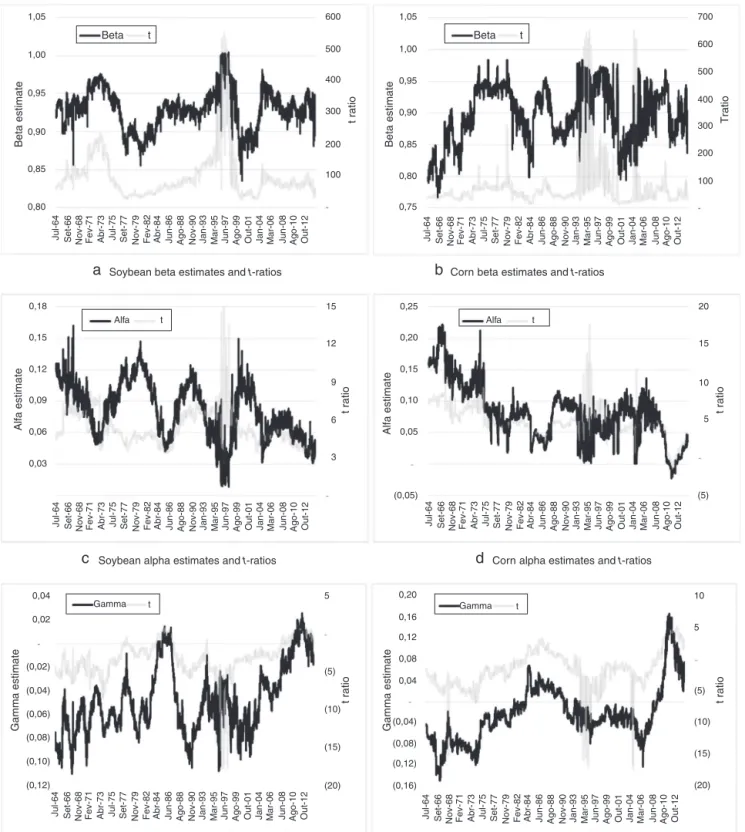
Fig.3.Rollingcoefficientestimatesforsoybeansandcorn.

estimates,whicharediscussedasfollows,provideamore com-prehensiveanalysisoftheseissuesandshedmorelightonthe analysis.

Fig.3showstheevolutionofrollingα1,βandγcoefficient

estimateswitharollingwindowof1008observationsforcorn andsoybeansandtheir correspondingt-ratios fromJuly1963 toDecember2014.In general,rolling β coefficientestimates

forcornandsoybeanmodelsareinthe0.8–1.0rangeandare statisticallydistinguishablefromzero,whichindicatesgreater long-run shock persistence. Forcorn, β coefficient estimates present lowerlevels andhigherinstabilitythanthe respective soybeanparameter(Table5).

Withrespecttorollingα1coefficientestimates,which

(12)

Table5

Descriptivestatisticsforrollingα1,βandγcoefficientestimatesandhalf-life

period.

Summarystatistics

Mean Median SD

Alpha(α1)

Soybeans 0.0796 0.0786 0.0265

Corn 0.0792 0.0774 0.0458

p-Value 0.3689 0.0000 0.0000

Beta(β)

Soybeans 0.9314 0.9329 0.0262

Corn 0.9004 0.9012 0.0453

p-Value 0.0000 0.0000 0.0000

Gamma(γ)

Soybeans −0.0480 −0.0524 0.0279

Corn −0.0228 −0.0285 0.0526

p-Value 0.0000 0.0000 0.0000

Half-life(ϑ)

Soybeans 65.94 21.24 2276.53

Corn 98.47 56.52 2827.86

p-Value 0.3123 0.0000 0.0000

forsoybeanand0–0.20forcorn(Fig.3).Inaddition,rollingα coefficientestimatesfor cornandsoybeansseemedtopresent similarlevels,alongwithhighervariabilityforcorn(Table5). Finally,rollingγcoefficientestimatesforsoybeans(corn)vary between−0.10and0.02(−0.15and0.15).Theγestimatesfrom thecornmodelalsoshowhighervaluesandgreatervariability thantheestimatesfromthesoybeanmodel.Ingeneral,sincethe coefficientisusuallynegative,thereisevidenceofaninventory effect.

Furthermore,AppendicesA–Cpresenttherollingcoefficient estimates for seasonality andtime-to-maturity effects for the soybean andcorn markets. Results point tothe existence of greatervolatilityduringtheplantingperiodandbeforethe har-vestinthe U.S.(second andthirdquarters).The evolutionof time-to-maturitycoefficientindicateshigherfuturesprice vari-ability whenthefuturescontractapproachesitsexpiration for bothmarkets.

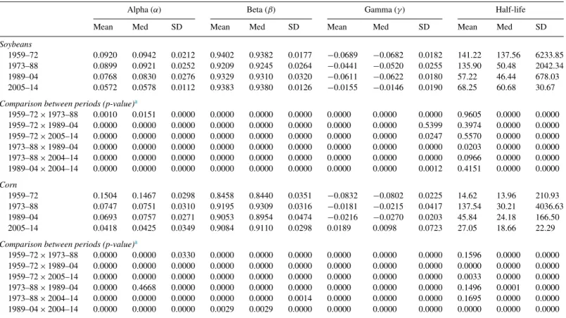
Table6showsthedescriptivestatisticsforrollingα1,βand

γ coefficient estimatesfor each separateperiod.The findings confirm previousresultsrelatedtolowerαestimatesoverthe last twoperiods,resulting inadecrease inthe importance of short-run volatility persistence in soybean and cornmarkets. Consequently,itcanbelargelyverifiedthatthelong-run persis-tence(α1+γ/2+β)andhalf-lifeperiodtendtobelowerinthe

Table6

Descriptivestatisticsforrollingα,βandγcoefficientestimatesandhalf-lifeperiodduring1959–1972,1973–1988,1989–2004,and2005–2014.

Alpha(α) Beta(β) Gamma(γ) Half-life

Mean Med SD Mean Med SD Mean Med SD Mean Med SD

Soybeans

1959–72 0.0920 0.0942 0.0212 0.9402 0.9382 0.0177 −0.0689 −0.0682 0.0182 141.22 137.56 6233.85

1973–88 0.0899 0.0921 0.0252 0.9209 0.9245 0.0264 −0.0441 −0.0520 0.0255 135.90 50.48 2042.34

1989–04 0.0768 0.0830 0.0276 0.9329 0.9310 0.0320 −0.0611 −0.0622 0.0180 57.22 46.44 678.03

2005–14 0.0572 0.0578 0.0112 0.9383 0.9380 0.0126 −0.0155 −0.0146 0.0190 68.25 60.68 30.67

Comparisonbetweenperiods(p-value)a

1959–72×1973–88 0.0010 0.0151 0.0000 0.0000 0.0000 0.0000 0.0000 0.0000 0.0000 0.9605 0.0000 0.0000

1959–72×1989–04 0.0000 0.0000 0.0000 0.0000 0.0000 0.0000 0.0000 0.0000 0.5399 0.3974 0.0000 0.0000

1959–72×2005–14 0.0000 0.0000 0.0000 0.0000 0.0000 0.0000 0.0000 0.0000 0.0247 0.5570 0.0000 0.0000

1973–88×1989–04 0.0000 0.0000 0.0000 0.0000 0.0000 0.0000 0.0000 0.0000 0.0000 0.0203 0.0000 0.0000

1973–88×2004–14 0.0000 0.0000 0.0000 0.0000 0.0000 0.0000 0.0000 0.0000 0.0000 0.0966 0.0000 0.0000

1989–04×2004–14 0.0000 0.0000 0.0000 0.0000 0.0000 0.0000 0.0000 0.0000 0.0012 0.4151 0.0000 0.0000

Corn

1959–72 0.1504 0.1467 0.0298 0.8458 0.8440 0.0351 −0.0832 −0.0802 0.0225 14.62 13.96 210.93

1973–88 0.0747 0.0751 0.0310 0.9195 0.9309 0.0316 −0.0181 −0.0215 0.0417 137.54 30.21 4036.63

1989–04 0.0693 0.0757 0.0271 0.9053 0.8954 0.0474 −0.0216 −0.0270 0.0203 45.84 24.18 166.50

2005–14 0.0418 0.0425 0.0349 0.9084 0.9110 0.0298 0.0189 0.0098 0.0723 27.05 18.66 22.29

Comparisonbetweenperiods(p-value)a

1959–72×1973–88 0.0000 0.0000 0.0330 0.0000 0.0000 0.0000 0.0000 0.0000 0.0000 0.1596 0.0000 0.0000

1959–72×1989–04 0.0000 0.0000 0.0000 0.0000 0.0000 0.0000 0.0000 0.0000 0.0000 0.0000 0.0000 0.0000

1959–72×2005–14 0.0000 0.0000 0.0000 0.0000 0.0000 0.0000 0.0000 0.0000 0.0000 0.0033 0.0000 0.0000

1973–88×1989–04 0.0000 0.4668 0.0000 0.0000 0.0000 0.0000 0.0000 0.0000 0.0000 0.1496 0.0001 0.0000

1973–88×2004–14 0.0000 0.0000 0.0000 0.0000 0.0000 0.0014 0.0000 0.0000 0.0000 0.1695 0.0000 0.0000

1989–04×2004–14 0.0000 0.0000 0.0000 0.0029 0.0029 0.0000 0.0000 0.0000 0.0000 0.0000 0.0000 0.0000

(13)

recentperiod,especiallyduring2005–2014,despiteincreasing valuesforγ.

Conclusions

Agriculturalmarketsarelargelycharacterizedbyhighprice volatility,duetothelowpriceelasticityof supply.This char-acteristichighlightsthe risk of thisactivity, whichrepresents asusceptibilityfactorforprimaryproducingcountries.During thefirst decade ofthe 2000s, majoragriculturalcommodities experiencedasharpandrapidriseinpriceandvolatility,thus stimulatingdiscussionsandresearchinordertounderstandthe reasonsthatledtosuchascenario.Withtheincreaseinbiofuel productionfromgrainsandoilseedsandrestrictionofacreage growthduetoenvironmentalissues,thepressureonagricultural areaswillintensify,whichmaybereflectedinincreasingfood prices.

Studiesthat investigate pricevolatility patterns in agricul-turalmarketshavesignificantimportance,sincetheycanhelpto improvedecision-makingprocessesrelatedtoproduction,risk managementandmarketing.Inaddition,policymakerscanalso benefitfromthesestudiesastheyanalyzetheimpactsofenergy policies on agricultural price and food security. This paper contributestotherecentdebateaboutvolatilityinagricultural marketsbyfocusingtheanalysisongrainvolatilitypersistence andtheinventoryeffect.Usingaconditionalvolatilitymodelto generaterollingestimates,thisworkprovidesevidenceonthe evolutionofvolatility, itspersistence andtheinventory effect overthelast40years.Inaddition,thestudyevaluatesthe matu-rityandseasonalityeffectsthroughmodelestimates.

Results indicate that the three most significant volatility peaksingrainmarketsoccurredin1973(collapseofthe Bret-ton Woods system), 1988 (large production shortfallin U.S. grain markets) and 2008 (subprime crisis). High persistence from shocks on the conditional variance was found in corn and soybean markets between 1959 and 2014. There is also evidence of an asymmetric effect of volatility shocks in the grainmarkets,withnegativeshocksexhibitingalargerimpact on conditional variance. In addition, the evolution of rolling coefficient estimates indicates decreasing short-run volatility persistenceinbothmarketsinrecentyears.Consequently, long-run persistence and the half-life period fall slightly. Further, seasonalityandtime-to-maturityeffectsarealsofoundinboth markets.

Intermsoffutureworks,thistopiccanbefurtherexplored with the inclusion of othercommodities, along withthe use of other volatility models. Volatility spillover effects over timecouldalsobe analyzedbymeansof recursiveparameter estimates of multivariate GARCH models. In addition, other variablescanbeincludedinthemodel,suchasfuturescontract tradingvolumeandcropreportannouncements.

Conflictsofinterest

Theauthorsdeclarenoconflictsofinterest.

Acknowledgements

TheauthorswouldliketothankFAPESP(SãoPauloResearch Foundation)forthefinancialsupportgiventothisresearch.

(14)

(15)

AppendixC. Rollingtime-to-maturitycoefficientestimatesforsoybeansandcorn

References

Allen,D.E.,&Cruickshank,S.N.(2000).EmpiricaltestingoftheSamuelson

hypothesis:AnapplicationtofuturesmarketsinAustralia,Singaporeand theUK.Workingpaper.SchoolofFinanceandBusinessEconomics,Edith CowanUniversity.

Anderson,R.W.(1985).Somedeterminantsofthevolatilityoffuturesprices.

JournalofFuturesMarkets,5,331–348.

Arezki,R.,Lederman,D.,&Zhao,H.(2014).Therelativevolatilityof

com-modityprices:Areappraisal.AmericanJournalofAgriculturalEconomics,

96(3),939–951.

Arezki, R., Hadri, K., Loungani, P., & Rao, Y. (2014). Testing the

Prebisch–Singerhypothesissince1650:Evidencefrompaneltechniques thatallowformultiplebreaks.JournalofInternationalMoneyandFinance,

42,208–223.

Arezki,R.,Loungani,P.,Ploeg,R.,&Venables,A.J.(2014).Understanding

internationalcommoditypricefluctuations.JournalofInternationalMoney andFinance,42,1–8.

Balcombe,K.(2009).Thenatureanddeterminants ofvolatilityin

agricul-turalprices:Anempiricalstudyfrom1962–2008.AreporttotheFoodand AgricultureOrganizationoftheUnitedNations.

Beckmann,J.,&Czudaj,R.(2014).Volatilitytransmissioninagriculturalfutures

markets.EconomicModelling,36,541–546.

Bellemare,M.F.,Barrett,C.B.,&Just,D.R.(2013).Thewelfareimpactsof

commoditypricevolatility:EvidencefromruralEthiopia.AmericanJournal ofAgriculturalEconomics,95(4),877–899.

Bessembinder,H.,&Seguin,P.J.(1993).Pricevolatility,tradingvolume,and

marketdepth:Evidence fromfuturesmarkets.JournalofFinancialand QuantitativeAnalysis,28(1),21–39.

Blattman,C.,Hwang,J.,&Williamson,J.G.(2007).Winnersandlosersinthe

commoditylottery:Theimpactoftermsoftradegrowthandvolatilityinthe Periphery1870–1939.JournalofDevelopmentEconomics,82(1),156–179.

Calvo-Gonzalez,O.,Shankar,R.,&Trezzi,R.(2010).Arecommodityprices

morevolatilenow?WorldBankPolicyResearchWorkingPaper5460.

Carpantier, J.-F. (2010). Commodities inventory effect. Discussion Paper

2010/40.Belgium:CenterforOperationsResearchandEconometrics, Uni-versitéCatholiquedeLouvain,Louvain-la-Neuve.

Carpantier,J.-F.,&Dufays, A.(2012).Commodities volatilityandthe

the-oryofstorage.DiscussionPaper2012/37.Belgium:CenterforOperations ResearchandEconometrics,UniversitéCatholiquedeLouvain, Louvain-la-Neuve.

Carpantier,J.-F.,&Samkharadze,B.(2013).Theasymmetriccommodity

inven-toryeffectontheoptimalhedgeratio.JournalofFuturesMarkets,33(9), 868–888.

Chatrath,A.,Adrangi,B.,&Dhanda,K.K.(2002).Arecommodity prices

chaotic?AgriculturalEconomics,27,123–137.

Daal,E.,Farhat,J.,&Wei,P.P.(2006).Doesfuturesexhibitmaturityeffect?

NewevidencefromanextensivesetofUSandforeignfuturescontracts.

ReviewofFinancialEconomics,15(2),113–128.

Dawson,P.J.(2015).Measuringthevolatilityofwheatfuturespricesonthe

LIFFE.JournalofAgriculturalEconomics,66(1),20–35.

Du,X.,Yu,C.L.,&Hayes,D.J.(2011).Speculationandvolatilityspillover

inthecrudeoilandagriculturalcommoditymarkets:ABayesiananalysis.

EnergyEconomics,33(3),497–503.

Duong,H.N.,&Kalev, P.S.(2008).TheSamuelson hypothesisin futures

markets:Ananalysisusingintradaydata.JournalofBanking&Finance,

32(4),489–500.

Ghoshray,A.(2013).Dynamicpersistenceofprimarycommodityprices.

Amer-icanJournalofAgriculturalEconomics,95(1),153–164.

Gilbert,C.L.(2010).Howtounderstandhighfoodprices.Journalof

Agricul-turalEconomics,61,398–425.

Gilbert,C.L., &Morgan,C.W. (2010).Foodprice volatility.

Philosophi-calTransactionsoftheRoyalSocietyB:BiologicalSciences,365(1554), 3023–3034.

Glauber,J.W.,&Heifner,R.G.(1986).Forecastingfuturespricevariability.

Appliedcommoditypriceanalysis,forecasting,andmarketrisk manage-ment.InProceedingsoftheNCR134conference(pp.153–165).

Goodwin,B.K.,&Schnepf,R.(2000).Determinantsofendogenouspricerisk

incornandwheatfuturesmarkets.JournalofFuturesMarkets,20,753–774.

Gupta,S.K.,&Rajib,P.(2012).Samuelsonhypothesis&Indiancommodity

derivativesmarket.Asia-PacificFinancialMarkets,19(4),331–352.

Hasan,M.Z.,Akhter,S.,&Rabbi,F.(2013).Asymmetryandpersistenceof

energypricevolatility.InternationalJournalofFinanceandAccounting,

2(7),373–378.

He,L.-Y.,Yang,S.,Xie,W.-S.,&Han,Z.-H.(2014).Contemporaneousand

asymmetricpropertiesintheprice–volumerelationshipsinChina’s agricul-turalfuturesmarkets.EmergingMarketsFinanceandTrade,50,148–166.

Headey,D.,&Fan,S.(2008).Anatomyofacrisis:Thecausesandconsequences

ofsurgingfoodprices.AgriculturalEconomics,39,375–391.

Hennessy,D.A.,&Wahl,T.I.(1996).Theeffectsofdecisionmakingonfutures

pricevolatility.AmericanJournalofAgriculturalEconomics,78,591–603.

Hováth,R.,&Sapov,B.(2016).GARCHmodels,tailindexesanderror

distri-butions:Anempiricalinvestigation.NorthAmericanJournalofEconomics andFinance,37,1–15.

Huchet-Bourdon, M. (2011). Agricultural commodity price volatility: An

overview.OECDfood, agricultureand fisheriespapers, no.52.OECD Publishing.

Hudson,D.,&Coble,K.(1999).Harvestcontractpricevolatilityforcotton.

Isengildina,O.,Irwin,S.H.,&Good,D.L.(2006).ThevalueofUSDAsituation

(16)

Jacks,D.S.,O’Rourke,K.H.,&Williamson,J.G.(2011).Commodityprice volatilityandworldmarketintegrationsince1700.ReviewofEconomics andStatistics,93(3),800–813.

Kalev,P.S.,&Duong,H.N.(2008).AtestoftheSamuelsonhypothesisusing

realizedrange.JournalofFuturesMarkets,28,680–696.

Karali,B.(2012).DoUSDAannouncementsaffectcomovementsacross

com-modityfuturesreturns?JournalofAgriculturalandResourceEconomics,

37,77–97.

Karali,B.,&Power,G.J.(2013).Short-andlong-rundeterminantsof

com-moditypricevolatility.AmericanJournalAgriculturalEconomics,95(3), 724–738.

Karali,B.,&Thurman,W.N.(2010).Componentsofgrainfuturesprice

volatil-ity.JournalofAgriculturalandResourceEconomics,35(2),167–182.

Karali,B.,Dorfman,J.H.,&Thurman,W.N.(2010).Deliveryhorizonand

grainmarketvolatility.JournalofFuturesMarkets,30,846–873.

Kenyon,D.,Kling,K.,Jordan,J.,Seale,W.,&McCabe,N.(1987).Factors

affectingagriculturalfuturespricevariance.JournalofFuturesMarkets,7, 73–92.

Khan,B.F.(2014).Determinantsoffuturespricevolatilityofstorable

agricul-turalcommodities:Thecaseofcotton(ThesisinAgriculturalandApplied Economics).TexasTechUniversity.

Khoury,N.,&Yourougou,P.(1993).Determinantsofagriculturalfuturesprice

volatilities:Evidence fromWinnipeg Commodity Exchange.Journalof FuturesMarkets,13,345–356.

Kocagil,A.E.,&Shachmurove,Y.(1998).Return-volumedynamicsinfutures

markets.JournalofFuturesMarkets,18,399–426.

Malliaris, A.G.,& Urrutia,J. L. (1998).Volume and pricerelationships:

Hypothesesandtestingforagriculturalfuture.JournalofFuturesMarkets,

18(4),399–426.

Mensi,W.,Beljid,M.,Boubaker,A.,&Managi,S.(2013).Correlationsand

volatilityspilloversacrosscommodityandstockmarkets:Linkingenergies, food,andgold.EconomicModelling,32,15–22.

Milonas,N.T.(1986).Pricevariabilityandthematurityeffectinfuturesmarkets.

Naylor,R.L.,&Falcon,W.P.(2010).Foodsecurityinaneraofeconomic

volatility.PopulationandDevelopmentReview,36(4),693–723.

Nazlioglu,S.,Erdem,C.,&Soytas,U.(2013).Volatilityspilloverbetweenoil

andagriculturalcommoditymarkets.EnergyEconomics,36,658–665.

Pockhilchuck,K.A.,&Savel’ev,S.A.(2016).Onthechoice ofGARCH

parametersforefficientmodellingofrealstockpricedynamics.Physica A:StatisticalMechanicsandApplications,448,248–253.

Power,G.J.,&Robinson,J.R.C.(2013).Commodityfuturespricevolatility,

convenienceyieldandeconomicfundamentals.AppliedEconomicsLetters,

20(11),1089–1095.

Prebisch,R.(1950).TheeconomicdevelopmentofLatinAmericaandits

prin-cipalproblems.EconomicBulletinforLatinAmerica,7,1–22.

Rapsomanikis,G.,&Sarris,A.(2008).Marketintegrationanduncertainty:The

impactofdomesticandinternationalcommoditypricevariabilityonrural householdincomeandwelfareinGhanaandPeru.JournalofDevelopment Studies,44(9),1354–1381.

Rutledge,D.J.S.(1976).Anoteonthevariabilityoffuturesprices.Reviewof

EconomicsandStatistics,58(1),118–120.

Serra, T. (2011). Volatility spillovers between food and energy

mar-kets: A semiparametric approach. Energy Economics, 33(6), 1155–1164.

Singer,H.(1950).Thedistributionofgainsbetweeninvestingandborrowing

countries.AmericanEconomicReview,11,473–485.

Smith,A.(2005).Partiallyoverlappingtimeseries:Anewmodelfor

volatil-itydynamicsincommodityfutures.JournalofAppliedEconometrics,20, 405–422.

Stigler,M.,&Prakash,A.(2011).Theroleoflowstocksingeneratingvolatility

andpanic.InA.Prakash(Ed.),Safeguardingfoodsecurityinvolatileglobal markets(pp.314–328).Rome:FoodandAgricultureOrganizationofthe UnitedNations(FAO).

Streeter,D.H.,&Tomek,W.G.(1992).Variabilityinsoybeanfuturesprices:

Anintegratedframework.JournalofFuturesMarkets,12,705–728.

Sumner, D. A. (2009). Recent commodity price movements in

histori-cal perspective. American Journal of Agricultural Economics, 91(5), 1250–1256.

Verma,A.,&Kumar,C.V.R.S.V.(2010).Anexaminationofthematurityeffect

intheIndiancommoditiesfuturesmarket.AgriculturalEconomicsResearch Review,23,335–342.

Vivian, A., & Wohar, M. E. (2012). Commodity volatility breaks.

Jour-nal of International Financial Markets, Institutionsand Money, 22(2), 395–422.

Watkins, C., & Mcaleer, M. (2008). How has volatility in metals

mar-kets changed? Mathematics and Computers in Simulation, 78(2–3), 237–249.

Wright,B.D.(2011).Theeconomicsofgrainpricevolatility.AppliedEconomic

PerspectivesandPolicy,33(1),32–58.

Yang,J.,Balyeat,R.B.,&Leatham,D.J.(2005).Futurestradingactivityand

commoditycashpricevolatility.JournalofBusinessFinance&Accounting,

32,297–323.

Yang,S.R.,&Brorsen,B.W.(1993).Nonlineardynamicsofdailyfutures

prices:Conditionalheteroskedasticityorchaos?JournalofFuturesMarkets,

13,175–191.

Zakoian,J.M.(1994).Thresholdheteroskedasticitymodels.Journalof