The Possibility of Primordial
Black Hole Direct Detection
Jos´
e Laurindo de G´
ois N´
obrega Sobrinho
Thesis submitted to obtain the PhD degree in
Mathematics
(speciality of Mathematical–Physics)
Supervisor:
Pedro Manuel Edmond Reis da Silva Augusto
The Possibility of Primordial
Black Hole Direct Detection
Jos´
e Laurindo de G´
ois N´
obrega Sobrinho
Thesis presented and unanimously approved in public session,
on 20 June 2011, to obtain the PhD Degree in Mathematics
(speciality of Mathematical–Physics)
Jury
Chairman:
Rector of the Universidade da Madeira
Members of the Committee
(in alphabetical order)
:
Doctor Anne Marie Green
Associate Professor, University of Nottingham, United Kingdom
Doctor Carlos Paulo da Cˆ
amara Crawford do Nascimento
Professor Auxiliar com Agrega¸c˜ao, Universidade de Lisboa
Doctor Jos´
e Pizarro de Sande e Lemos
Professor Associado com Agrega¸c˜ao, Universidade T´ecnica de Lisboa
Doctor Pedro Manuel Edmond Reis da Silva Augusto
x
Abstract
This thesis explores the possibility of directly detecting blackbody emission from Primordial Black Holes (PBHs). A PBH might form when a cosmological density fluctuation with wavenumberk, that was once stretched to scales much larger than the Hubble radius during inflation, reenters inside the Hubble radius at some later epoch. By modeling these fluctuations with a running–tilt power–law spectrum (n(k) = n0 +a1(k)n1 +a2(k)n2 +a3(k)n3; n0 = 0.951; n1 = −0.055; n2 and n3
unknown) each pair (n2,n3) gives a different n(k) curve with a maximum value
(n+) located at some instant (t+). The (n+,t+) parameter space [(1.20,10−23 s) to
(2.00,109 s)] has t
+ = 10−23 s–109 s and n+ = 1.20–2.00 in order to encompass the
formation of PBHs in the mass range 1015 g–1010M
⊙ (from the ones exploding at present to the most massive known). It was evenly sampled: n+every 0.02; t+ every
order of magnitude. We thus have 41×33 = 1353 different cases. However, 820 of these (≈ 61%) are excluded (because they would provide a PBH population large enough to close the Universe) and we are left with 533 cases for further study.
Although only sub–stellar PBHs (≪ 1M⊙) are hot enough to be detected at large distances we studied PBHs with 1015 g–1010M
⊙ and determined how many might have formed and still exist in the Universe. Thus, for each of the 533 (n+,t+) pairs
we determined the fraction of the Universe going into PBHs at each epoch (β), the PBH density parameter (ΩP BH), the PBH number density (nP BH), the total number of PBHs in the Universe (N), and the distance to the nearest one (d). As a first result,≈14% of these (72 cases) give, at least, one PBH within the observable Universe, one–third being sub–stellar and the remaining evenly spliting into stellar, intermediate mass and supermassive. Secondly, we found that the nearest stellar mass PBH might be at 32 pc, while the nearest intermediate mass and supermassive PBHs might be 100 and 1000 times farther, respectively.
Finally, for 6% of the cases (four in 72) we might have substellar mass PBHs within 1 pc. One of these cases implies a population of∼105 PBHs, with a mass of∼1018 g
(similar to Halley’s comet), within the Oort cloud, which means that the nearest PBH might be as close as∼103 AU. Such a PBH could be directly detected with a
probability of∼10−21 (cf. ∼10−32 for low–energy neutrinos). We speculate in this
possibility.
x
Resumo
Esta tese explora a possibilidade de detetar diretamente a emiss˜ao de corpo negro de Buracos Negros Primordiais (BNPs). Um BNP pode formar-se quando uma flutua¸c˜ao de densidade cosmol´ogica de n´umero de onda k, esticada para uma escala muito superior ao raio de Hubble durante a infla¸c˜ao, reentra dentro do raio de Hubble numa ´epoca posterior. Modelando estas flutua¸c˜oes com um espectro da forma n(k) = n0 +a1(k)n1 +a2(k)n2 +a3(k)n3 (n0 = 0.951; n1 = −0.055; n2 e
n3 desconhecidos), cada par (n2,n3) d´a lugar a uma curva n(k) com um m´aximo
(n+) localizado num determinado instante (t+). O espa¸co de parˆametros (n+,t+)
[(1.20,10−23 s) a (2.00,109 s)] tem t
+ = 10−23 s–109 s e n+ = 1.20–2.00 de forma
a incluir a forma¸c˜ao de BNPs na gama de 1015 g–1010M
⊙ (desde os que est˜ao a explodir no presente aos maiores conhecidos). Fez-se uma amostragem uniforme:
n+ em passos de 0.02;t+ para todas as ordens de magnitude. Ficamos, assim, com
41×33 = 1353 casos diferentes. Contudo, 820 destes (≈61%) foram exclu´ıdos (pois dariam lugar a uma popula¸c˜ao de BNPs suficiente para fechar o Universo) sobrando 533 casos para estudo posterior.
Embora apenas os BNPs de massa subestelar (≪ 1M⊙) sejam suficientemente quentes para que possam ser detetados a grandes distˆancias, estudamos BNPs com 1015 g–1010M
⊙ e determinamos quantos podem ter-se formado e continuar a existir no Universo. Assim, para cada um dos 533 pares (n+,t+) determinamos a fra¸c˜ao
do Universo convertida em BNPs em cada ´epoca (β), a densidade num´erica de BNPs (nP BH), o n´umero total de BNPs no Universo (N) e a distˆancia para o mais pr´oximo (d). Um primeiro resultado sugere que ≈14% destes (72 casos) d˜ao, pelo menos, um BNP no Universo observ´avel, sendo um ter¸co subestelares e os restantes igualmente distribu´ıdos pelos estelares, de massa interm´edia e supermassivos. Al´em disso, o BNP estelar mais pr´oximo poder´a estar a 32 pc enquanto que o de massa interm´edia e supermassivo mais pr´oximos podem estar, respectivamente, 100 e 1000 vezes mais distantes.
Finalmente, para 6% dos casos (quatro em 72) podemos ter BNPs de massa subeste-lar a distˆancias inferiores a 1 pc. Um destes casos d´a-nos uma popula¸c˜ao de∼ 105
BNPs com ∼ 1018 g (semelhante ao cometa Halley) dentro da nuvem de Oort, o
que significa que o BNP mais pr´oximo pode estar a ∼ 103 AU. Tal BNP pode ser
detetado diretamente com uma probabilidade de ∼ 10−21 (cf. ∼ 10−32 no caso de
neutrinos de baixa energia). Especulamos sobre esta possibilidade.
List of Figures xv
List of Tables xix
List of Equations xxi
Acronyms xxvii
Physical Constants and Parameters xxix
Conventions xxx
Preface xxxv
1 Introduction: PBHs and the Early Universe 1
1.1 The Primordial Universe . . . 3
1.1.1 Relativistic Cosmology preliminaries . . . 3
1.1.2 Inflation . . . 9
1.1.3 The Lambda–Cold Dark Matter Model . . . 13
1.1.4 The scale factor . . . 16
1.1.5 Fluctuations . . . 20
1.1.6 Degrees of freedom . . . 22
1.2 Cosmological phase transitions . . . 28
1.2.1 The QCD phase transition . . . 29
1.2.2 The EW phase transition . . . 38
1.2.3 The electron–positron annihilation epoch . . . 38
1.3 The primordial power spectrum . . . 39
1.3.1 Scale–free power law spectrum . . . 40
1.3.2 Running–tilt power–law spectrum . . . 43
1.4 PBH formation . . . 44
1.4.1 The condition for PBH formation . . . 44
1.4.2 PBH initial mass . . . 45
1.4.3 PBHs from collapsing density perturbations . . . 46
1.4.4 The fraction of the Universe going into PBHs . . . 47
1.4.5 The PBH density parameter . . . 52
1.5 This thesis . . . 54
2 Duration of the cosmological phase transitions 59 2.1 QCD phase transition . . . 59
2.2 EW phase transition . . . 64
2.2.1 Crossover (SMPP) . . . 64
2.2.2 Bag Model (MSSM) . . . 67
2.3 Electron–positron annihilation . . . 70
3 Fluctuations and phase transitions 73
3.1 QCD phase transition . . . 73
3.1.1 Bag Model . . . 73
3.1.2 Lattice Fit . . . 78
3.1.3 Crossover . . . 79
3.2 EW phase transition . . . 81
3.2.1 Crossover (SMPP) . . . 81
3.2.2 Bag Model (MSSM) . . . 81
3.3 Fluctuations during the e+e− annihilation . . . 82
4 The threshold δc for PBH formation 83 4.1 QCD Bag Model . . . 83
4.2 QCD Crossover . . . 87
4.3 QCD Lattice Fit . . . 93
4.4 EW Crossover (SMPP) . . . 99
4.5 EW Bag Model (MSSM) . . . 103
4.6 Electron–positron annihilation . . . 104
5 The fraction of the Universe going into PBHs 109 5.1 Scale–free power law spectrum . . . 109
5.2 Running–tilt power–law spectrum . . . 110
5.3 The different scenarios . . . 112
5.4 Radiation–dominated universe . . . 115
5.5 EW Crossover . . . 118
5.6 Electron–positron annihilation . . . 118
5.7 QCD phase transition . . . 121
5.8 EW phase transition (MSSM) . . . 132
6 The PBH density parameter 137 6.1 The present day value of the PBH density parameter . . . 137
6.2 The distance to the nearest PBH . . . 138
6.3 Supermassive PBHs . . . 140
6.4 The effect of the electron–positron annihilation . . . 142
6.5 The effect of the QCD phase transition . . . 147
6.5.1 Bag Model . . . 147
6.5.2 Lattice Fit . . . 149
6.5.3 Crossover . . . 155
6.6 The effect of the EW phase transition (MSSM) – Bag Model . . . 158
6.7 Intermediate–mass PBHs . . . 162
6.8 Stellar mass PBHs . . . 163
6.9 Sub–stellar mass PBHs . . . 163
6.10 PBHs and CDM . . . 166
6.11 Nearby PBHs . . . 167
7.3 Radiation . . . 180
7.4 The QCD phase transition (tU ∼10−4 s) . . . 181
7.5 The EW phase transition - Bag Model (tU ∼10−10 s) . . . 184
7.6 Electron–positron annihilation (tU ∼1 s) . . . 186
7.7 Simultaneous contributuions (EW and QCD) . . . 187
7.8 The most interesting cases . . . 187
7.9 Can we directly detect PBHs? . . . 189
7.10 Summary . . . 192
8 Conclusions 197 8.1 Where are we now? . . . 197
8.2 Where can we go? . . . 199
A The Universe Timeline 201 B The Cosmic Microwave Background temperature 206 C The Standard Model of Particle Physics 211 D The Minimal Supersymmetric extension of the SMPP 219 E The EW phase transition 227 F The quantum–to–classical transition 233 G PBHs from collapsing density perturbations 235 G.1 PBHs from cosmological phase transitions . . . 238
G.2 Evolution of subcritical perturbations . . . 240
H The threshold for PBH formation (variable δc) 241 H.1 QCD Bag Model . . . 241
H.2 QCD Crossover . . . 241
H.3 QCD Lattice Fit . . . 241
H.4 EW Crossover (SMPP) . . . 247
H.5 EW Bag Model (MSSM) . . . 247
H.6 Electron–positron annihilation . . . 247
I The parameters δc1 and δc2 250
J The parameter ∆T and the EW Crossover 255
K The values of n2 and n3 when n+ = 1.4 258
L The maximum value of σ2(t
k) for different cases 260
M The peaks of the curve β(tk) 262
O The minimum distance d(t0, tk) 273
P On the possibility of direct detection of BHs by electromagnetic
radiation: fundamentals 282
P.1 Black Hole Thermodynamics . . . 282
P.2 The Schwarzschild Black Hole . . . 282
P.3 Secondary γ–rays from BHs . . . 283
P.4 The possibility of direct detection of BHs . . . 285
P.5 Present technical limitations to the possibility of direct detection of BHs . . . 286
P.5.1 Radio . . . 286
P.5.2 Infrared . . . 291
P.5.3 Visible . . . 291
P.5.4 Ultraviolet . . . 295
P.5.5 X–Rays . . . 298
P.5.6 γ–rays . . . 301
P.5.7 Black Holes in their Terminal Phases . . . 301
P.5.8 Emission of Massive Particles and Secondary γ–rays . . . 301
P.5.9 Summary . . . 304
P.6 Discussion and conclusions . . . 305
1 The PBH mass spectrum . . . 2
2 The effective number of degrees of freedom g(T). . . 28
3 Naive phase diagram of strongly interacting matter. . . 30
4 Behaviour of the temperature as a function of the scale factor during a first–order QCD transition. . . 32
5 The entropy density of hot QCD relative to the entropy density of an ideal QGP. . . 35
6 Energy density and pressure as functions of T /Tc for the QCD tran-sition in LGT. . . 36
7 The square of the speed of sound as a function of T /Tc for the QCD transition in LGT. . . 37
8 The relative abundance of PBHs formed at some epoch . . . 54
9 The beginning and the end of the QCD phase transition (Bag Model and Lattice Fit). . . 60
10 The sound speed as a function of T /Tc during the QCD transition according to the Lattice Fit model. . . 61
11 The square of the speed of sound for the QCD Crossover. . . 62
12 The sound speed for the QCD phase transition (Bag Model). . . 63
13 The sound speed for the QCD phase transition (Lattice Fit). . . 64
14 The sound speed for the QCD phase transition (Crossover). . . 65
15 The scale factor during the QCD transition as a function of time. . . 65
16 The sound speed for the EW Crossover as a function of temperature. 66 17 The minimum value attained by the sound speed as a function of the parameter ∆T (EW Crossover and QCD Crossover). . . 67
18 The sound speed for the EW phase transition (Bag Model). . . 69
19 The scale factor as a function of time. . . 69
20 The sound speed during the electron–positron annihilation as a func-tion of temperature. . . 71
21 Regions in the (δk, log10x) plane corresponding to different classes of perturbations (QCD Bag Model). . . 78
22 Regions in the (δk, log10x) plane corresponding to different classes of perturbations (QCD Lattice Fit). . . 80
23 PBH formation (QCD Bag Model; x= 2; δc = 1/3). . . 84
24 PBH formation (QCD Bag Model; x= 15, x= 30, x= 90; δc = 1/3). 85 25 The curve in the (x, δ) plane indicating which values lead to collapse to a PBH (QCD Bag Model; x >1; δc = 1/3). . . 86
26 PBH formation (QCD Bag Model; x = 0.927, x = 0.6, x = 0.308; δc = 1/3). . . 88
27 The curve in the (x, δ) plane indicating which values lead to collapse to a PBH (QCD Bag Model; y−1 < x <1;δ c = 1/3). . . 89
28 PBH formation (QCD Bag Model; x = 0.26, x = 0.22, x = 0.11; δc = 1/3). . . 90
29 The curve in the (x, δ) plane indicating which values lead to collapse to a PBH (QCD Bag Model; x < y−1;δ
c = 1/3). . . 91
30 The curve in the (x, δ) plane indicating which values lead to the formation of a PBH (QCD (full) Bag Model; δc = 1/3). . . 91
31 The same as Figure 30 but now with δ=δ(log10(tk/1 s)). . . 92
32 PBH formation (QCD Crossover; δc = 1/3). . . 94
33 The curve in the (log10(tk/1s), δ) plane indicating which parameter values lead to collapse to a PBH (QCD Crossover; δc = 1/3). . . 95
34 PBH formation (QCD Lattice Fit; x= 15; δc = 1/3). . . 97
35 PBH formation (QCD Lattice Fit; x= 2; δc = 1/3). . . 98
36 Regions in the (δk, log10x) plane corresponding to the different classes of perturbations (QCD Lattice Fit). . . 99
37 PBH formation (QCD Lattice Fit; x= 25, x= 50; δc = 1/3). . . 100
38 PBH formation (QCD Lattice Fit; x= 0.985, x= 0.871; δc = 1/3). . . 101
39 PBH formation (QCD Lattice Fit; x= 0.70, x= 0.47; δc = 1/3). . . . 102
40 The curve in the (log10(tk/1s), δ) plane indicating which values lead to collapse to a PBH (QCD Lattice Fit; δc = 1/3). . . 103
41 PBH formation during the EW Crossover when δc = 1/3. . . 104
42 The curve in the (log10(tk/1s), δ) plane indicating which values lead to the formation of a PBH (EW Crossover; δc = 1/3). . . 105
43 The curve indicating which values lead to collapse to a PBH (EW transition within the MSSM; δc = 1/3). . . 106
44 PBH formation during the cosmological electron–positron annihila-tion when δc = 1/3. . . 107
45 The curve on the (log10(tk/1s), δ) plane indicating which values lead to collapse to a BH during the cosmological electron–positron anni-hilation when δc = 1/3. . . 107
46 α2(t k) for a scale–free power law spectrum with n = 0.951 . . . 110
47 n(k) with a maximum located atk+ = 7.1×10⁻¹⁷m−1 . . . 111
48 α2(t k) for the running–tilt power–law spectrum whenn(k+) = 1.4 . . 112
49 α2(t k) for the running–tilt power–law spectrum when the spectral index presents a maximum at k+ = 1.1×10⁻¹⁶ m−1 . . . 112
50 σ2(t k) for the running–tilt power–law spectrum when n(k+) = 1.4 . . 113
51 σ2(t k) for the running–tilt power–law spectrum when the spectral index presents a maximum at k+ = 1.1×10⁻¹⁶ m−1 . . . 113
52 Observational constraints on β(tk) . . . 116
53 β(tk) for a radiation–dominated universe when n+ = 1.30. . . 117
54 β(tk) for a radiation–dominated universe near the cut–off linetk= 105 s.126 55 β(tk) during the EW Crossover . . . 127
56 β(tk) during the electron–positron annihilation epoch (examples). . . 128
57 β(tk) when n+ = 1.56 and t+ = 10−1 s . . . 129
58 β(tk) when n+ = 1.54 and t+ = 10−2 s . . . 129
59 β(tk) when n+ = 1.48 and t+ = 10−4 s . . . 130
60 β(tk) when n+ = 1.52 and t+ = 10−3 s . . . 130
62 β(tk) when n+ = 1.36 andt+= 10−9 s. . . 132
63 β(tk) during the EW phase transition (examples) . . . 134
64 β(tk) with simultaneous contributions from the EW and QCD phase transitions . . . 135
65 d(t0, tk) whenn+= 1.34 and t+ = 10−8 s . . . 140
66 The PBH mass spectrum and SMBHs (1) . . . 144
67 The PBH mass spectrum and SMBHs (2) . . . 145
68 The PBH mass spectrum during the electron–positron annihilation (examples I) . . . 146
69 The PBH mass spectrum during the electron–positron annihilation (examples II) . . . 147
70 The PBH mass spectrum when n+= 1.70 andt+= 102 s. . . 147
71 The PBH mass spectrum for the QCD Bag Model . . . 150
72 The PBH mass spectrum for the QCD Bag Model (n+ = 1.58, t+ = 10−1 s) . . . 152
73 The PBH mass spectrum for the QCD Bag Model (n+ = 1.40, t+ = 10−8 s) . . . 152
74 The PBH mass spectrum for the QCD Lattice Fit . . . 153
75 The PBH mass spectrum for the QCD Lattice Fit when n+ = 1.42 and t+= 10−6 s . . . 154
76 The PBH mass spectrum for the QCD Lattice Fit when n+ = 1.42 and t+= 10−7 s . . . 154
77 The PBH mass spectrum due to the QCD Crossover when n+ = 1.50 and t+= 10−3 s . . . 155
78 The PBH mass spectrum due to the QCD Crossover (cases with ΩP BH ∼10−5) . . . 157
79 The PBH mass spectrum due to the EW (ΩP BH ∼10−1) . . . 160
80 The PBH mass spectrum due to the EW when n+ = 1.34 and t+ = 10−12 s . . . 160
81 The PBH mass spectrum due to the EW when n+ = 1.44 and t+ = 10−6 s . . . 161
82 The PBH mass spectrum due to the EW and the QCD . . . 162
83 The PBH mass spectrum when n+ = 1.30 and t+ = 10−16 s; n+ = 1.36 andt+= 10−11 s. . . 164
84 The PBH mass spectrum when n+ = 1.28 and t+ = 10−18 s; n+ = 1.32 andt+= 10−14 s . . . 165
85 The PBH mass spectrum when n+= 1.38 andt+= 10−9 s . . . 165
86 ΩP BH(tk) whenn+= 1.34 andt+= 10−11 s . . . 167
B-1 The CMB anisotropy map . . . 206
B-2 The theoretical CMB anisotropy power spectrum. . . 209
B-3 The Lyman α forest (quasarRDJ030117 + 002025) . . . 210
C-1 The particle content of the SMPP. . . 213
D-1 Mass spectrum of supersymmetric particles and the Higgs boson ac-cording to the SPS1a scenario. . . 222
E-2 Evolution of the Higgs potential for different values of temperature. . 231
G-1 Shapes of the critical perturbations . . . 236
G-2 The fluid element worldlines for a mexican–hat perturbation during PBH formation . . . 237
G-3 The evolution of a mexican–hat perturbation . . . 237
G-4 Time evolution of a near–critical polynomial perturbation . . . 238
G-5 Time evolution of an overcritical Gaussian perturbation . . . 238
G-6 PBH formation during a first–order phase transition. . . 239
G-7 Time evolution of an undercritical Gaussian perturbation . . . 240
H-1 PBH formation (QCD Bag Model;x= 2, x= 15, x= 30; δc assumes different values). . . 242
H-2 PBH formation (QCD Bag Model; x= 0.927, x= 0.6, x= 0.308; δc assuming different values). . . 243
H-3 PBH formation (QCD Bag Model; x = 0.26, x = 0.22, x = 0.11; δc assumes different values). . . 244
H-4 The curve in the (x, δ) plane indicating which values lead to collapse to a PBH (QCD Bag Model; x >1; δc = 1/3 and δc = 0.7). . . 245
H-5 The curve in the (x, δ) plane indicating which values lead to collapse to a PBH (QCD Bag Model; y−1 < x <1; δ c = 1/3 and δc = 0.7). . . 245
H-6 The curve in the (x, δ) plane indicating which values lead to collapse to a PBH (QCD Bag Model; x < y−1;δ c = 1/3 and δc = 0.7). . . 246
H-7 The curve in the (log10(tk/1s), δ) plane indicating which values lead to collapse to a PBH (QCD Crossover). . . 246
H-8 The curve in the (log10(tk/1s), δ) plane indicating which values lead to collapse to a PBH (QCD Lattice Fit; δc = 0.7). . . 247
H-9 The curve in the (log10(tk/1s), δ) plane indicating which values lead to collapse to a PBH (EW Crossover; δc = 1/3 and δc = 0.7). . . 248
H-10 The curve in the (log10(tk/1s), δ) plane indicating which values lead to collapse to a PBH (EW transition within the MSSM; δc = 0.7). . . 248
H-11 The curve on the (log10(tk/1s), δ) plane indicating which values lead to collapse to a PBH in the case of the cosmological electron–positron annihilation when δc = 1/3 and when δc = 0.7. . . 249
J-1 The curve (1−f)δc for the EW Crossover when δc = 1/3. . . 257
M-1 β(tk) when n+ = 1.36 and t+ = 10−7 s. . . 264
P-1 Luminosity per unit frequency as a function of rs . . . 288
P-2 Maximum distance for detecting the Hawking radiation (radio) . . . . 292
P-3 Maximum distance for detecting the Hawking radiation (infrared) . . 294
P-4 Maximum distance for detecting the Hawking radiation (visible) . . . 295
P-5 Maximum distance for detecting the Hawking radiation (UV) . . . 298
P-6 Maximum distance for detecting the Hawking radiation (X–rays) . . . 300
1 The best fit values for the ΛCDM model . . . 15
2 The evolution of the number of degrees of freedom g(T) in the Uni-verse according to the SMPP . . . 26
3 The wavenumberkfor the fluctuation crossing the horizon at different epochs . . . 52
4 The width of the QCD phase transition according to the Bag Model, Lattice Fit and Crossover when Tc = 170 MeV . . . 64
5 The Scale Factor for different instants of time . . . 70
6 The reduction of the sound speed value during the electron–positron annihilation. . . 71
7 The width of the cosmological electron–positron annihilation in terms of time as a function of the parameter ∆T . . . 72
8 Classes of fluctuations for the QCD first–order phase transition . . . 74
9 Classes of fluctuations for the EW first–order phase transition . . . . 81
10 The different scenarios concerning the calculation of β . . . 115
11 The cases for which β > 10−100 for a radiation–dominated universe with a running–tilt power–law spectrum when δc = 1/3 . . . 119
12 The contribution to β from the electron–positron annihilation epoch . 120 13 The contribution to β from the QCD Bag Model . . . 122
14 The contribution to β from the QCD Lattice Fit . . . 123
15 The contribution to β from the QCD Crossover . . . 124
16 The contribution to β from the EW Bag Model . . . 133
17 The relation ΩP BH(tk)/β(tk) for different values of σ2(tk) and δc . . . 138
18 The cases giving SMBHs . . . 141
19 The contribution to ΩP BH from the electron–positron annihilation epoch . . . 143
20 The contribution to ΩP BH from the QCD Bag Model . . . 148
21 The contribution to ΩP BH from the QCD Lattice Fit . . . 151
22 The contribution to ΩP BH from the QCD Crossover . . . 156
23 The contribution to ΩP BH from the EW Bag Model . . . 159
24 IMBHs and PBHs . . . 162
25 SBHs and PBHs . . . 169
26 The contribution to ΩP BH from SSBHs . . . 170
27 SSBHs and PBHs . . . 172
28 CDM and PBHs . . . 173
29 Global statistics for the different scenarios . . . 178
30 The different contributions (per scenario) giving N ≥1 . . . 179
31 The most interesting cases from the observational point of view . . . 191
A-1 The Universe timeline . . . 205
C-1 The three lepton families of the SMPP . . . 212
C-2 The three quark families of the SMPP . . . 212
C-3 Fundamental Bosons within the SMPP . . . 214
C-4 Mesons . . . 216
C-5 Baryons . . . 218
D-1 The SMPP particles and their supersymmetric MSSM partners . . . . 220
D-2 The MSSM particles in terms of gauge eigenstates and mass eigenstates223 D-3 Mass spectrum of the supersymmetric particles and the Higgs boson according to the SPS1a scenario . . . 224
D-4 The number of degrees of freedom for each kind of particle within the MSSM . . . 225
D-5 The evolution of the number of degrees of freedom g(T) in the Uni-verse according to the MSSM (SPS1a scenario) . . . 226
I-1 The evolution of δc1 and δc2 for the QCD Bag Model . . . 251
I-2 The evolution of δc1 for the QCD Crossover . . . 251
I-3 The evolution of δcA, δc1 and δc2 for the QCD Lattice Fit . . . 252
I-4 The evolution of δc1 for the EW Crossover . . . 253
I-5 The evolution of δc1 and δc2 for the EW Bag Model . . . 253
I-6 The evolution of δc1 for the cosmological electron–positron annihila-tion with ∆T = 0.115Tc and δc = 1/3 . . . 254
J-1 The lowest value of δc1,min for the EW Crossover with δc assuming different values . . . 256
K-1 The values of n2 and n3 which give n+= 1.4 . . . 259
L-1 The maximum value of σ2(t k) for different cases . . . 261
M-1 Peaks of the curve β(tk) in the case n+ = 1.36 and t+ = 10−7 s . . . . 263
M-2 The fraction of the Universe going into PBHs during radiation dom-ination and during cosmological phase transitions . . . 265
N-1 The cases for which β > 10−100 for a radiation–dominated universe with a running–tilt power–law spectrum when δc = 0.7 . . . 272
O-1 The distance to the nearest PBH . . . 274
P-1 Emission of neutrinos and leptons by BHs . . . 285
P-2 Telescopes . . . 287
P-3 Sensitivities for the UBVR filters (Johnson) . . . 288
P-4 List of 50 Schwarzschild BHs . . . 289
P-5 Maximum distances for BH detection at the radio wavelengths . . . . 290
P-6 Maximum distances for BH detection at the infrared wavelengths . . 293
P-7 Maximum distances for BH detection at the visible wavelengths . . . 296
P-8 Maximum distances for BH detection at the UV wavelengths . . . 297
P-9 Maximum distances for BH detection at the X–rays wavelengths . . . 299
P-10 Maximum distances for BH detection at the γ–ray wavelengths . . . . 303
P-11 Evaporation times for Schwarzschild BHs . . . 304
List of Equations
1 Friedmann–Lemaˆıtre–Robertson–Walker metric . . . 4
2 Friedmann–Lemaˆıtre equation (energy equation) or Friedmann equation . 4 3 Friedmann–Lemaˆıtre equation (motion equation) . . . 4
4 First Law of Thermodynamics for the expanding Universe . . . 5
5 Equation of state of the Universe . . . 5
6 Isentropic sound speed . . . 5
7 The background value of the sound speed for a radiation–dominated Universe 5 8 The density equation of the Universe . . . 6
9 The density of the Universe as a function of time . . . 6
10 Second Law of Thermodynamics (for a perfect fluid) . . . 6
11 Entropy density for a perfect fluid . . . 6
12 The isentropic sound speed from the entropy density . . . 6
13 The scale factor (R) . . . 6
14 Scale factor for a radiation–dominated Universe . . . 7
15 Scale factor for a matter–dominated Universe . . . 7
16 Scale factor for a dark energy–dominated Universe . . . 7
17 Radial null geodesic equation . . . 7
18 Redshift (z) . . . 8
19 Hubble parameter (H) . . . 8
20 Hubble radius (RH) . . . 8
21 Horizon mass (MH) . . . 9
22 The Friedmann equation and the Hubble parameter . . . 9
23 The critical density (ρc) . . . 9
24 Matter density parameter (Ωm) . . . 9
25 Curvature density parameter (Ωκ) . . . 9
26 Cosmological Constant density parameter (ΩΛ) . . . 9
27 The Friedmann equation as a sum of density parameters . . . 9
28 The scale factor and inflation . . . 11
29 The number of e–folds elapsed during inflation . . . 11
30 The inflaton energy density . . . 12
31 The inflaton pressure density . . . 12
32 The energy equation for the inflaton . . . 12
33 The motion equation for the inflaton . . . 12
34 The slow–roll approximation . . . 13
35 The present day value of the Hubble parameter (H0) . . . 15
36 The value of the cold dark matter density parameter (ΩCDM) . . . 16
37 The value of the Cosmological Constant density parameter . . . 16
38 The cosmological constant (Λ) . . . 16
39 The normalization of the scale factor . . . 16
40 Scale factor and redshift . . . 16
41 The Hubble parameter for a radiation–dominated Universe . . . 17
42 The Hubble parameter for a matter–dominated Universe . . . 17
43 The Hubble parameter for a dark energy–dominated Universe . . . 17
44 The Hubble parameter during inflation . . . 17 45 The scale factor fortSN ≤t≤t0 . . . 17
46 The scale factor forteq ≤t≤tSN . . . 17 47 The scale factor fortQCD+ ≤t≤teq . . . 17 48 The scale factor fortQCD− ≤t≤tQCD+ . . . 18
49 The scale factor fortEW+ ≤t≤tQCD− . . . 18 50 The scale factor fortEW− ≤t≤tEW+ . . . 18
51 The scale factor forte ≤t≤tEW− . . . 18 52 The scale factor forte ≤t≤teq (simplified) . . . 19 53 Temperature, scale factor and redshift . . . 19 54 The age of the Universe (t0) . . . 19
55 Density fluctuation . . . 21 56 The horizon crossing time tk . . . 21 57 The evolution of a perturbed region . . . 22 58 The evolution of a perturbed region and the density contrastρk . . . 22 59 Generalized blackbody distribution . . . 23 60 The particle number density of particles of a particular species . . . 23 61 The energy density of particles of a particular species . . . 23 62 The effective number of degrees of freedom at a particular epoch (SMPP) 24 63 The effective number of degrees of freedom for T >172.5 GeV (SMPP) . 25 64 The effective number of degrees of freedom at a particular epoch (MSSM) 27 65 The effective number of degrees of freedom for T >172.5 GeV (MSSM) . 27 66 Latent heat for the quenched lattice QCD . . . 30 67 First–order phase transition strenght . . . 30 68 Pressure coexistence condition . . . 31 69 The pressure for the QGP . . . 33 70 The pressure for the HG . . . 33 71 The bag constant . . . 33 72 The energy density for the QGP . . . 34 73 The energy density for the HG . . . 34 74 The energy density during the QCD phase transition as a function of time 34 75 The relation between the latent heat and the bag constant . . . 34 76 The entropy density for the QCD Bag Model . . . 35 77 The step function Θ . . . 35 78 The entropy density for the QCD Lattice Fit model . . . 37 79 The sound speed for the QCD Lattice Fit model . . . 37 80 The entropy density for the QCD Crossover model . . . 38 81 The sound speed for the QCD Crossover model (as a function of temperature) 38 82 The quantityδ2
H(k, t) (time independent in superhorizon scales) . . . 39 83 Power–law spectrum for the primordial density fluctuations . . . 41 84 Power–law spectrum at the horizon crossing time . . . 41 85 Power–law spectrum at the horizon crossing time (normalized) . . . 41 86 The expression giving Γ(ω) . . . 41 87 The relation betweenδ2
H(k) andδH(kc) evaluated at some pivot scalekc . 41 88 The expression giving δ2
89 The expression giving δ2
H(kc) (numerical) . . . 42 90 The relation between δ2
H(k) and δH(kc) evaluated at the pivot scale kc = 0.002Mpc−1 . . . 42 91 Power–law spectrum with a running spectral index . . . 43 92 The running of the spectral index –n(k) . . . 43 93 The observational values ofn0 and n1 . . . 43
94 The condition for PBH formation . . . 45 95 The scaling relation for the PBH mass . . . 46 96 The probability that a region of mass m has a density contrast in the
range [δ, δ+dδ] . . . 47 97 The fraction of the Universe going into PBHs . . . 48 98 The fraction of the Universe going into PBHs whenδc ≫σ(tk) . . . 48 99 Top–hat window function . . . 49 100 The mass variance of the primordial density fluctuations . . . 49 101 The mass variance and the cut–off in k–space . . . 49 102 The mass variance and δ2
H(k, t) . . . 49 103 The relation betweenσ2(t
k) andα2(k) . . . 50 104 The expression giving α2(k) . . . 50
105 The expression giving α2(k) in the case of a power–law spectrum . . . 51
106 The relation between the wavelengthk and the pivot scale kc . . . 51 107 The mass variance in terms of masses . . . 52 108 The mass variance for the Harrison–Zeldovich spectrum . . . 52 109 The PBH density parameter at a given epoch – ΩP BH(tk) . . . 53 110 ΩP BH(tk) and the PBH mass scaling relation . . . 53 111 The PBH mass spectrum on the differential form . . . 53 112 PBH maximum mass . . . 54 113 The relation between ΩP BH(t0, tk) and ΩP BH(tk) . . . 54 114 The scale factor at the end of the QCD (Bag Model or Lattice Fit) as a
relation of temperatures . . . 59 115 The expression giving the scale factor at the end of the QCD (Bag Model
or Lattice Fit) . . . 59 116 The instanttQCD+ (the end of the QCD Bag Model or Lattice Fit) . . . . 59
130 The scale factor at the end of the EW Bag Model as a relation of temper-atures . . . 67 131 The expression giving the scale factor at the end of the EW Bag Model . 68 132 The instanttEW+ (the end of the EW Bag Model) . . . 68
133 Expansion of the universe during the EW Bag Model phase transition (∆R) 68 134 The expression giving the scale factor at the beginning of the EW Bag
Model . . . 68 135 The instanttEW− (the beginning of the EW Bag Model) . . . 68 136 The sound speed during the e+e− annihilation epoch (as a function of
temperature) . . . 70 137 The minimum value of the sound speed during thee+e− annihilation epoch 70 138 The sound speed during thee+e− annihilation epoch (as a function of time) 71 139 The parameter x . . . 73 140 The parameter y . . . 73 141 The density at the beginning of the QCD Bag Model – ρ(tQCD−) . . . 73 142 The parameter x as a function of time (QCD Bag Model) . . . 74 143 The value of the parameter y for the QCD Bag Model . . . 74 144 The evolution of the density contrast in a perturbed region . . . 74 145 The density at horizon crossing – ρ(tk) . . . 75 146 The evolution of a perturbed region and the adiabatic index . . . 75 147 The turnaround point (the instant at which PBH formation starts) . . . . 75 148 The turnaround point for fluctuations of classes A and F . . . 75 149 The turnaround point for fluctuations of class D . . . 75 150 The relationKs/Kk for fluctuations of class B . . . 75 151 The relationKs/Kk for fluctuations of class E . . . 76 152 The relationKs/Kk for fluctuations of class C . . . 76 153 Scale factor for the perturbed region at the beginning of a first–order
phase transition – S1 . . . 76
154 The relation betweenS1, S2 and the parameter y . . . 76
155 An expression for S2 suitable for fluctuations of class E . . . 76
156 An expression for S2 suitable for fluctuations of class F . . . 76
157 The turnaround point for fluctuations of class B . . . 76 158 The turnaround point for fluctuations of class C . . . 77 159 The turnaround point for fluctuations of class E . . . 77 160 The separation between classes A,B,C and classes D,E . . . 77 161 The separation between classes D,E and class F . . . 77 162 The separation between classes A and B . . . 77 163 The separation between classes B and C . . . 77 164 The separation between classes D and E . . . 77 165 The separation between classes C and D . . . 77 166 The value of the parameter y for the QCD Lattice Fit . . . 79 167 The relation between the scale factor at horizon crossing and at the
170 The relation betweentk and tc for the QCD Crossover . . . 80 171 The parameter x as a function of time (EW Bag Model) . . . 81 172 The threshold for PBH formation during a cosmological phase transition . 83 173 The function f for fluctuations of class A within the QCD Bag Model . . 83 174 The function f for fluctuations of class B within the QCD Bag Model . . 83 175 The function f for fluctuations of class C within the QCD Bag Model . . 83 176 The function f for fluctuations of class E within the QCD Bag Model . . 83 177 The function f for fluctuations of class F within the QCD Bag Model . . 83 178 The function αsp . . . 87 179 The function f for the QCD Crossover . . . 89 180 The elementary volumedS3 . . . 89
181 The elementary volumedS3 for the QCD Crossover . . . 89
182 The function f for the QCD Crossover in terms of tk and tc . . . 92 183 The function f for the QCD Crossover as a function of tk . . . 92 184 The functionf =fALat for fluctuations of classAwithin the QCD Lattice
Fit . . . 93 185 The elementary volumedS3 for the QCD Lattice Fit . . . 95
186 The function fALat as a function of time . . . 95
187 The function f for fluctuations of class B within the QCD Lattice Fit . . 95 188 The function fBLat . . . 96
189 The function fBLat as a function of time . . . 96
190 The function f for fluctuations of class C within the QCD Lattice Fit . . 96 191 The function fCLat . . . 96
192 The function fCLat as a function of time . . . 96
193 The expansion of the running–tilt power–law spectrum (up toi= 3) . . . 110 194 β(tk) for a Crossover–like transition . . . 113 195 β(tk) for a Crossover–like transition and the contribution from radiation
–βRad(tk) . . . 114 196 ΩP BH(tk) and the PBH mass scaling relation (II) . . . 137 197 ΩP BH(tk) simplified . . . 137 198 The relation between ΩP BH(tk) andβ(tk) . . . 137 199 The relation between ΩP BH(t0, tk) and β(tk) . . . 137 200 The present day value of the PBH density parameter – ΩP BH(t0) . . . 138
201 The present day value of the PBH number density –nP BH(t0) . . . 139
202 The distance to the nearest PBH formed at a particular epoch – d(t0, tk) . 139 B-1 The CMB temperature . . . 206 E-1 The potential of the scalar fieldφ – EW phase transition . . . 229 E-2 The temperature T0 – EW phase transition . . . 230
E-3 The temperature T∗ – EW phase transition . . . 230 E-4 The temperature Tc – EW phase transition . . . 231 F-1 The quantum–to–classical transition effectiveness . . . 233 F-2 The quantum–to–classical transition effectiveness as a function of the PBH
Acronyms
2dFGRS– 2 degree Field Galaxy Redshift Survey
ACBAR– Arcminute Cosmology Bolometer Array Receiver
AMSB– Anomaly–Mediated Susy Breaking
AGILE – Astro–revilatore Gamma a Immagini LEggero
BH– Black Hole
CBI – Cosmic Background Imager
CDM – Cold Dark Matter
CMB– Cosmic Microwave Background
EoS– Equation of State
EW– ElectroWeak
FUSE– Far Ultraviolet Spectroscopic Explorer
FLRW – Friedmann–Lemaˆıtre–Robertson–Walker
GALLEX– GALLium EXperiment
GMSB– Gauge–Mediated Susy Breaking
GUT – Grand Unification Theory
HDM – Hot Dark Matter
HESS – High Energy Stereoscopic System
HG– Hadron Gas
HST– Hubble Space Telescope
IIE– Innovative Interstellar Explorer
IMBH– Intermediate Mass Black Hole (102M
⊙ < MBH <106M⊙)
INTEGRAL– INTErnational Gamma–Ray Astrophysics Laboratory ΛCDM – Lambda–Cold Dark Matter Model
LEP – Large Electron Positron collider
LGT– Lattice Gauge Theory
LHC – Large Hadron Collider
LSP– Lightest Supersymmetric Particle
LSS– Large Scale Structure
LTE– Local Thermodynamic Equilibrium
MSSM– Minimal Supersymmetric extension of the Standard Model
XMM– X–ray Multi–mirror Mission.
PBH– Primordial Black Hole
PDG – Particle Data Group
QCD – Quantum ChromoDynamics
QGP– Quark–Gluon Plasma
RHIC – Relativistic Heavy Ion Collider
SBH – Stellar mass Black Hole (1M⊙≤MBH ≤102M⊙)
SDSS – Sloan Digital Sky Survey
SLC – Stanford Linear Collider
SMBH – SuperMassive Black Hole (MBH ≥106M⊙)
SMPP – Standard Model of Particle Physics
SOFIA– Stratospheric Observatory For Infrared Astronomy
SPS – Snowmass Points and Slopes
SST – Spitzer Space Telescope
SSBH– Sub–Stellar mass Black Hole (10−5g< M
BH <1M⊙)
SUSY – SUperSYmmetry
VLA– Very Large Array
WIMP – Weakly Interacting Massive Particle
Physical Constants and Parameters
(∗)Speed of light c 2.99792458×10⁸ ms−1
Planck constant h 6.6260755(40)×10−34 Js
Gravitation constant G 6.67259(85)×10−11 m3kg−1s−2
Boltzmann constant k 1.380658(12)×10−23 JK−1
Electron charge e 1.60217733(49)×10−19 C
Planck mass mP 2.17671(14)×10−8 kg Planck length lP 1.61605(10)×10−35 m Planck time tP 5.39056(34)×10−44 s
Astronomical Unit AU 1.4959787066×10¹¹ m
Parsec pc 3.0856776×10¹⁶ m
Solar mass M⊙ 1.9891×1030 kg Jupiter mass mJ 1.8987×1027 kg Earth mass mT 5.9742×1024 kg
Pluto orbital semi–major axis 39.5 AU
Radius of the Oort Cloud ≈0.4 pc (†)
Distance to the galactic centre 8.5 kpc Radius of the galactic halo 16 kpc(‡)
Distance to the Large Magellanic Cloud (LMC) 55 kpc Distance to the Andromeda galaxy (M31) 0.725 Mpc Size of the Observable Universe 1026 m (⋄)
(*) The values were taken from Cox (2000), except otherwise noted. For some of the values the standard error of the last digits follows in parentheses.
(†) Dones et al. (2004).
(‡) We considered, in our integrations, the radius of the galactic halo approximately equal to the radius of the galactic disc (e.g. Uns¨old & Bascheck, 2002).
Conventions
α – relation between the mass variance and δH;
αsp – ratio of the sound speed with respect to the background value (1/
√
3) at a given moment;
β – the fraction of the Universe going into PBHs;
δ – fluctuation amplitude;
δk – fluctuation amplitude at the horizon crossing time;
δc – the threshold for PBH formation;
δc1 – the threshold for PBH formation at the beginning of a phase transition;
δc2 – the threshold for PBH formation at the end of a phase transition;
κ – spatial curvature of the observable Universe; Λ – cosmological constant;
ω – adiabatic index;
ρ – density of the overdense region; ¯
ρ – Universe average density;
ρ0 – Universe density at the present time;
ρ1, ρ2 – density of the overdense region, respectively, at the beginning and at the
end of a first–order phase transition;
ρc – critical density;
ρHG – HG density;
ρQGP – QGP density;
ρk – density at the horizon crossing time;
ρP BH – PBH mass density;
σ – mass variance;
Ωκ – curvature density parameter;
ΩΛ – cosmological constant density parameter;
Ωb – baryon density parameter; ΩCDM – CDM density parameter; Ωm – matter density parameter; ΩP BH – PBH density parameter; B – bag constant;
cs – sound speed;
cs0 – background sound speed for a radiation–dominated Universe;
d – the minimum distance to the nearest PBH;
f – the fraction of the overdense region spent in the dust–like phase;
fA,fB,fC,fE,fF – the functionf for fluctuations of classesA,B,C,E orF (QCD Bag Model);
fALat,fBLat,fCLat – the functionf for fluctuations of classesA,BorC (QCD Lattice
Fit model);
g – number of degrees of freedom;
g′
ep, gep – number of degrees of freedom, respectively, before and after the electron– positron annihilation epoch;
g′
gHG – number of degrees of freedom for the HG;
gQGP – number of degrees of freedom for the QGP;
H – Hubble parameter;
h– normalized Hubble constant (H0/100 kms−1Mpc−1);
H0 – Hubble constant;
k – wavenumber;
k+ – the wavenumber for which the power spectrum shows a maximum;
kc – pivot scale (the wavenumber at which the normalized scalar and tensor spectra cross);
ke – wavenumber at the end of inflation;
kr – wavenumber during radiation domination; l – latent heat;
MH – horizon mass;
MP BH – PBH mass; n – spectral index;
n+ – the maximum value of the power spectrum;
n0 – tilt of the spectrum for the running–tilt power–law spectrum;
n1 – running of tilt for the running–tilt power–law spectrum;
n2, n3 – unknown parameters (running–tilt power–law spectrum);
nP BH – PBH number density;
N – the number of PBHs within the observable Universe; P – primordial power spectrum for the density fluctuations; p – pressure;
pQGP – QGP pressure;
pHG – HG pressure; R – scale factor;
R0 – present day value of the scale factor (normalized to unity);
Rk – scale factor at the horizon crossing time;
RH – Hubble radius;
Rl – strength of a first–order phase transition;
RJ – Jeans length;
Rs – Schwarzschild radius;
S – the scale factor for the perturbed region;
S1, S2 – the scale factor for the perturbed region, respectively, at the beginning and
at the end of a first–order phase transition;
Sc – the scale factor for the perturbed region at the turnaround point;
s – entropy density;
sQGP – QGP entropy density;
sHG – HG entropy density;
t+ – the epoch at which the power spectrum attains its maximum value (n+);
tQCD−, tQCD+ – the age of the Universe, respectively, at the beginning and at the
end of the QCD;
t0 – the age of the Universe (present time);
t1 – beginning of the QCD Lattice Fit or QCD Crossover;
tc – turnaround point;
teq – the age of the Universe at radiation–matter equality;
tEW−, tEW+ – the age of the Universe, respectively, at the beginning and at the end
of the EW;
tH – Hubble time;
ti, te – the age of the Universe, respectively, at the beginning and at the end of inflation;
tk – horizon crossing time;
tSN – the age of the Universe at matter–Λ equality (i.e., the instant when the expan-sion of the Universe starts to accelerate according to the high redshift SuperNovae Ia data);
T – temperature;
T∗ – temperature at which the inflection point in the Higgs field appears;
T0 – present day background temperature;
Tc – critical temperature;
Non–negligible contributions to β (†):
B QCD Bag Model
BE QCD Bag Model and EW Bag Model BL QCD Bag Model or QCD Lattice Fit BLE (QCD Bag Model or QCD Lattice Fit)
and EW Bag Model
E EW Bag Model
ea e−e+ annihilation
L QCD Lattice Fit
R Radiation
RB Radiation and QCD Bag Model
RBE Radiation and QCD Bag Model and EW Bag Model RBea Radiation and QCD Bag Model and e−e+ annihilation
RBL Radiation and (QCD Bag Model or QCD Lattice Fit) RBLC Radiation and (QCD Bag Model or QCD Lattice Fit or
QCD Crossover)
RBLCE Radiation and (QCD Bag Model or QCD Lattice Fit or QCD Crossover) and EW Bag Model
RBLCea Radiation and (QCD Bag Model or QCD Lattice Fit or QCD Crossover) and e−e+ annihilation
RBLE Radiation and (QCD Bag Model or QCD Lattice Fit) and EW Bag Model
RC Radiation and QCD Crossover
RCea Radiation and QCD Crossover and e−e+ annihilation
RE Radiation and EW Bag Model Rea Radiation and e−e+ annihilation
RL Radiation and QCD Lattice Fit
RLea Radiation and QCD Lattice Fit and e−e+ annihilation
(†) We might also have situations with one or more contributions exceeding the observational limits (these are labeled with an∗). For example,RB∗LCE∗, represents a case for which we have,
besides the contribution from radiation R, contributions from the QCD Lattice Fit (L) or from the QCD Crossover (C). The QCD Bag Model is excluded due to observational constraints (B∗).
The same happens for the EW Bag Model (E∗). The contribution from the electron–positron
Preface
BHs are objects predicted by the Laws of Physics. They arise as a natural conse-quence of the Theory of General Relativity. Within the present day Universe we are aware of the processes that can lead to the formation of BHs with masses ranging from ∼ 1M⊙ up to ∼ 1010M⊙ and, in fact, in the past decades, we have identified
several BH candidates in all of these mass ranges. All those candidates were identi-fied by indirect means (i.e. measuring the effects they cause in their neighborhoods). The direct detection of a BH might be a giant step ahead in Astronomy and, in a more general sense, in Science itself.
According to Quantum Field Theory a BH should radiate like a black–body with a temperature inversely proportional to its own mass (i.e. smaller BHs are hotter than larger ones). The existence of this radiation, usually called Hawking radiation, could lead to the evaporation of the BH (if it is not balanced by the accretion of matter and radiation). During the evaporation process the BH emits electromagnetic waves (photons), neutrinos, gravitons and, in more advanced stages, electrons, positrons and other particles.
We decided to concentrate in the possible detection of the elecromagnetic compo-nent of this Hawking emission. In Sobrinho (2003)1 we have considered BHs of all
masses and determined the distances at which their electromagnetic emission can be detected at different wavelenghts using present day technology (i.e. the most sensitive telescopes operating at each electromagnetic spectrum band). As a result we found out that, for example, a BH with∼1016 g could be detected, inγ–rays, at a maximum distance of∼1010 m and that a BH with∼1018 g could be detected, in
X–rays, at a maximum distance of∼ 109 m. More massive BHs could be detected
in ultraviolet, visible, infrared and radio wavelengths but only within laboratorial distances (for example a BH with ∼1020 g could be detected, in the ultraviolet, at
a maximum distance of ∼106 m and a BH with ∼1026 g could be detected, in the
radio, at a maximum distance of ∼102 m).
Thus it seemed that, if one wanted to consider the realistic detection of the electro-magnetic radiation emitted by a BH then one should think of sub–stellar mass BHs (i.e. BHs with less than 1M⊙). As far as we know BHs with masses smaller than
≈3M⊙, cannot form in the present day Universe except, possibly, for the production of BHs in particle accelerators (in the speculative framework of branes) or, eventu-ally, when high–energy cosmic–rays collide with the upper layers of the atmosphere. However, at the beginning of the expansion of the Universe the same fluctuations that originated the observed structure of the present day Universe could have lead, also, to the production of BHs of all masses (i.e. ranging from the Planck mass up to∼1010M⊙). This BHs are called primordial BHs (PBHs) due to their origin.
Bearing in mind this idea we decided to enter deeper into Cosmology and deter-mine the PBH density in the present day Universe and, consequently, the minimum distance to the nearest PBH. In order to have a better picture of this early BH
mation epoch we decided to study not only the formation of sub–stellar mass PBHs but also the formation of PBHs of all masses.
This PhD thesis is organized as follows. In Chapter 1 we review several aspects about the early Universe and PBH formation that we found relevant for the present study. We finish this section with the expressions giving the fraction of the Universe going into PBHs at a given epoch and the PBH density parameter at that epoch as well as at the present day epoch. Being aware of the importance that cosmologi-cal phase transitions might have taken in PBH formation we have determined their location and duration within the Universe timeline. We do that, in Chapter 2, for the QCD phase transition, EW phase transition and electron–positron annihilation epoch. In Chapter 3 we consider the evolution of density fluctuations during cosmo-logical phase transitions adopting some results from the literature and deriving our own results whenever necessary. In Chapter 4 we determine the behaviour of the PBH formation threshold during the QCD phase transition, EW phase transition and electron–positron annihilation epoch. In Chapter 5 we determine, assuming a running–tilt power–law spectrum for the fluctuations, the fraction of the Universe going into PBHs at each epoch of interest. First we consider a radiation–dominated universe and then we show how the results are altered when one considers cosmologi-cal phase transitions. In Chapter 6 we determine the present day values for the PBH density parameter, their number density and the minimum distance to the nearest PBH of a given mass. We then compile the results taking into account the different cosmological phase transitions (QCD, EW and electron–positron annihilation) and the different kinds of BHs (with respect to their masses). Finally, in Chapter 7 we summarize and discuss the results and, in Chapter 8 we present our conclusions as well as some ideas for the future.
I have a graduation in Physics from the University of Madeira (1995). In 2003 I have completed my PAPCC (Provas de Aptid˜ao Pedag´ogica e Capacidade Cient´ıfica) that consisted on giving a lesson (Emula¸c˜ao da M´aquina URM no Mathematica) and defending an original thesis (Possibilidade de detec¸c˜ao directa de buracos negros por radia¸c˜ao electromagn´etica). In more than one sense this is equivalent to a M.Sc. thesis.
I am an Assistant at the recently created Centro de Ciˆencias Exactas e da Engen-haria (CCEE) in UMa. Prior to that, I have taught at the Departamento de F´ısica of the UMa (1995/97), at Escola Secund´aria de Jaime Moniz (1994/95, 1997/98), at Escola B´asica e Secund´aria de Machico (1998/99) and at the Departamento de Matem´atica (1999/2010) (later Departamento de Matem´atica e Engenharias, now incorporated into the new CCEE).
Depar-tamento de Matem´atica, I have started to work under the supervision of Professor Pedro Augusto on my PAPCC. The main objective was to determine the possibility of directly detecting BHs through their electromagnetic emission. I have concluded the PAPCC in 2003 and then I have started writing this PhD thesis on the same topic.
I am a founding member of theGrupo de Astronomia da Universidade da Madeira (GAUMa) created in 2000 in order to promote the research, outreach and teaching on Astronomy on Madeira. Since then I have been responsible and/or collabora-tor on many outreach activities in the area of Astronomy held here in Madeira (e.g. public/school lectures (about 30), observation sessions (about 20) hands–on activities with high school students (about 10), original posters (about 20)). An important mark in the Astronomy outreach in Madeira took place in 2009 with the International Year of Astronomy (IYA). I was an active member of the regional or-ganization for Madeira, coordenated by Prof. Pedro Augusto. Within the 365 days of 2009 we have organized 229 different events in Madeira (including the islands of Porto Santo and Desertas)!
This work would not have been possible without the constant support and under-standing from my wife Elda Maria Camacho Sobrinho and from our son Carlos Daniel Camacho Sobrinho. To them, that helped me in overcoming some of the most difficult moments, I dedicate this work. A special thanks to my parents who always supported me in my studies since the first day at school in October 1975 up to the present. I am also grateful to all relatives and colleagues who, in one way or another, helped me over these past years. In particular to my colleagues at the CCEE that were working on their own PhD thesis during these past years I would like to say that is was a pleasure and a privilege to share with them those high moments that only happen to those who endeavour in writing a PhD thesis in fundamental areas such as Mathematics and Physics. I am also deeply grateful to my supervisor (and colleague) Professor Pedro Augusto for his availability, support and advice during the writing up of this thesis.
This thesis was written in LaTeX. The numerical calculations were made using Mathematica 5.1 from Wolfram Research. All graphics and original figures were also generated with the help of Mathematica 5.1. I have chosen to work with Mathematica because it is the software that we use in the classes of Paradigmas da Programa¸c˜ao (an introductory computer programming course that I have been teaching since 1999).
Jos´e Laurindo de G´ois N´obrega Sobrinho
1
Introduction: PBHs and the Early Universe
Black Holes (BHs) are objects predicted by the laws of Physics. In fact, they arise as a natural consequence by solving the field equations of General Relativity. BHs with stellar mass can form through the collapse of the iron cores of massive stars, of mass M, after they have reached the end of their thermonuclear evolution (e.g. Misner et al., 1973). If the core radius shrinks to the so called Schwarzschild radius
Rs= 2GM
c2
then a BH is formed. The spherical surface formed at this radius is called the event horizon. As the matter continues to collapse inside the event horizon it will form a singularity (i.e., a point with infinite curvature and density where the theory of General Relativity should be replaced by a (still lacking) theory of Quantum Gravity). Inside the event horizon light is trapped.
Stellar mass BHs could have masses from three to hundreds of solar masses. How-ever, gravitational collapse allows for the formation of BHs with much greater or smaller masses (down to the Planck mass;∼ 10−5 g — e.g. Lemos (1996)). In the
centre of galactic nuclei gravitational collapse could lead to the formation of Super-Massive BHs (SMBHs). In fact, it is now well–established that SMBHs with masses in the range 106M⊙–1010M
⊙ reside in the centres of galaxies (e.g. Mack et al., 2007) including our own galaxy with a 4×10⁶M
⊙ SMBH (e.g. Gillessen et al., 2009).
Intermediate mass BHs (IMBHs), i.e., BHs with masses in the range 103M⊙–105M⊙,
might form either in the core of star clusters (e.g. Portegies Zwart et al., 2004) or galaxies (e.g. Greene & Ho, 2004).
As far as we know BHs with masses smaller than about 3M⊙, cannot form in the present Universe, except, possibly, for the production of BHs in accelerators such as the Large Hadron Collider (LHC) in the speculative framework of branes (e.g. Dimopoulos & Landsberg, 2001; Cavaglia et al., 2003) or, eventually, when cosmic– rays collide with the upper layers of the atmosphere (e.g. Anchordoqui et al., 2002).
However, the observed structure of the Universe on the scale of galaxies and smaller formations, requires that, at the beginning of the expansion of the Universe, there should have existed fluctuations which lead to the formation of such structures. It is plausible that some regions might have got so compressed that they did not continue to expand with the rest of the Universe but rather underwent gravitational collapse and produced Primordial Black Holes (PBHs). The first person to realize that was Hawking (1971)2.
-30 -20 -10 0 10
Log10Ht
1sL 10
20 30 40
Log
10
H
MH
1
g
L
Evaporated
Exploding
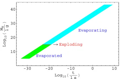
Evaporating
Figure 1: According to numerical simulations PBHs may form, at a given epoch, with masses ranging from 10−4
MH up to MH (Section 1.4.2). PBHs with initial masses smaller than 1015g should have completely evaporated by now, PBHs with≈1015
g should be exploding and those with initial masses greater than 1015
g are still evaporating or accreting matter (Sobrinho & Augusto, 2007).
PBHs with initial masses of order 1015g might be exploding right now (see Figure 1),
contributing to the γ–ray background (e.g. Page & Hawking, 1976; Carr, 1976; MacGibbon & Carr, 1991; Barrau, 1999).
PBHs are interesting for several reasons (e.g. Carr, 2005). For example, within the context of Cosmology, they can act as probes to scales which are many orders of magnitude smaller than the scales probed by Large Scale Structure (LSS) surveys andCosmic Microwave Background (CMB) angular anisotropy observations, giving the possibility to probe a very distinct part of the inflaton potential (e.g. Polarski, 2001) as well as the spectrum of primordial density fluctuations (e.g. Carr & Goymer, 1999). Within the context of Fundamental Physics they are the only BHs small enough for quantum emission effects to be important (e.g. MacGibbon & Carr, 1991) and thus they would play a key role in studying quantum gravitational effects. However, even if PBHs never formed, their nonexistence provides useful cosmological information (e.g. MacGibbon & Carr, 1991).
1.1
The Primordial Universe
1.1.1 Relativistic Cosmology preliminaries
According to observation we live in a flat, homogeneous and isotropic (on scales larger than 100 Mpc) expanding Universe (e.g. Jones & Lambourne, 2004). Thus, Cosmology, i.e. the study of the dynamical structure of the Universe as a whole, is based on the (e.g. d’Inverno, 1993)
Cosmological Principle – At each epoch, the Universe presents the same aspect from every point, except for local irregularities,
which is in essence, a generalization of the Copernican Principle that the Earth is not at the centre of the Solar System. We are assuming that there is a cos-mic time t with the Cosmological Principle valid for each spacelike hypersurface
t = const. The statement that each hypersurface has no privileged points means that it is homogeneous. The principle also requires that each hypersurface has no privileged directions about any point, i.e., the spacelike hypersurfaces are isotropic and necessarily spherically symmetric about each point. The concepts of homogene-ity and isotropy, however, do not apply to the Universe in detail (e.g. d’Inverno, 1993).
Assuming that there is a privileged class of observers in the Universe, namely, those associated with the smeared–out motion of the galaxies3, Weyl introduced a fluid
pervading space, which he called the substractum, in which the galaxies move like particles in a fluid. These ideas are contained in the (e.g. d’Inverno, 1993)
Weyl’s Postulate – The particles of the substractum lie in space–time on a con-gruence of timelike geodesics diverging from a point in the finite or infinite past.
The postulate requires that the geodesics do not intersect except at a singular point in the past and possibly at a similar singular point in the future. There is, therefore, one and only one geodesic passing through each point of space–time, and consequently the matter at any point possesses a unique velocity. This means that the substractum may be taken to be a perfect fluid. Although galaxies do not follow this motion exactly, the deviations appear to be random and less than one–thousandth of the velocity of light (e.g. d’Inverno, 1993).
Weyl’s postulate requires that the geodesics of the substractum are orthogonal to a family of spacelike hypersurfaces. We introduce coordinates (t, x1, x2, x3) such
that these spacelike hypersurfaces are given by constant t and such that the space coordinates (x1, x2, x3) are constant along the geodesics. Such coordinates are called
comoving coordinates (e.g. d’Inverno, 1993). Comoving observers are also called fundamental observers.
Relativistic Cosmology is based on three assumptions: (1) the Cosmological Princi-ple, (2) Weyl’s postulate and (3) General Relativity4.
A flat, homogeneous and isotropic expanding universe can be described by the Friedmann–Lemaˆıtre–Robertson–Walker (FLRW) metric (e.g. d’Inverno, 1993)
ds2 =dt2−R2(t)
dr2
1−κr2 +r
2 dθ2+sin2θdφ2
(1)
where R(t) is the so called scale factor which describes the time dependence of the geometry (the distance between any pair of galaxies, separated by more than 100 Mpc, is proportional to R(t)) and κ is a constant which fixes the sign of the spatial curvature (κ = 0 for Euclidean space, κ > 0 for a closed elliptical space of finite volume and κ < 0 for an open hyperbolic space). Notice that, whatever the physics of the expansion, the space–time metric must be of the FLRW form, because of the isotropy and homogeneity (e.g. Longair, 1998).
Considering the FLRW metric (1), Weyl’s postulate, General Relativity (with a cos-mological constant term Λ) and a comoving coordinate system it turns out that the field equations lead to two independent equations sometimes called the Friedmann– Lemaˆıtre equations (e.g. Yao et al., 2006; Uns¨old & Bascheck, 2002)
˙
R R
!2
= 8πGρ
3 −
κ R2 +
Λ
3 (2)
¨
R R =
Λ 3 −
4πG
3 (ρ+ 3p) (3)
where we have used relativistic units (c= 1) and a dot denotes differentiation with respect to cosmic time t. Equation (3) involves a second time derivative of R and so it can be regarded as an equation of motion, whereas equation (2), sometimes called theFriedmann equation, only involves a first time derivative ofR and so may be considered an integral of motion, i.e., an energy equation.
The addition of a cosmological constant term Λ is equivalent to assume that matter is not the only source of gravity. The Λ term was introduced by Einstein with the purpose of constructing a static cosmological model for the Universe. However, with the discovery of the expansion of the Universe (Slipher, 1917) the model became ob-solete. More recently, a Λ > 0 term was introduced again in order to account for the remarkable discovery that the expansion of the Universe is, in fact, accelerat-ing rather than retardaccelerat-ing (Section 1.1.3). Takaccelerat-ing into account that, accordaccelerat-ing to observation, we live in a flat universe, we consider κ= 0 (e.g. Yao et al., 2006).
Energy conservation leads to a third equation, which can also be derived from equa-tions (2) and (3), and is just a consequence of the First Law of Thermodynamics (e.g. Yao et al., 2006)
˙
ρ=−3R˙
R(ρ+p). (4)
We need also anequation of state (EoS) relating the pressurepto the energy density
ρat a given epoch. This relation is, in general, non–trivial. However, in Cosmology, where one deals with dilute gases, the EoS can be written in a simple linear form (e.g. Carr, 2003; Ryden, 2003)
p=wρ (5)
where the dimensionless quantity w is the so–called adiabatic index. Normally w
is a constant such that 0 ≤ w ≤ 1. If w = 0 we are in the case of a pressureless matter–dominated universe and, ifw= 1 we have a stiff EoS which may be the case if the Universe is dominated by ascalar field5 (e.g. Harada & Carr, 2005).
In the case of cosmological perturbations the radiation fluid behaves as a perfect (i.e. dissipationless) fluid, the entropy (S) in a comoving volume is conserved and, one has a reversible process. The isentropic6 sound speed can be written as (e.g.
Schmid et al., 1999)
c2s =
∂p ∂ρ
S
=w. (6)
In the early hot and dense primordial Universe it is appropriate to assume an EoS corresponding to a gas composed of radiation and relativistic massive particles with
w= 1/3 (e.g. Carr, 2003)
p= ρ 3
which means that, in the case of a radiation–dominated universe, the sound speed is given by
cs = 1
√
3. (7)
However, during inflation (Section 1.1.2) or in a universe dominated by a cosmolog-ical constant, w becomes negative and may not even be constant (e.g. Yao et al.,
5
A scalar field is a field that associates a scalar value to every point in space. On the other hand, a vector field associates a vector to every point in space. In Quantum Field Theory, a scalar field is associated with spin 0 particles (scalar bosons) and a vector field is associated with spin 1 particles (vector bosons).