AN EFFICIENT HYBRID HEURISTIC METHOD
FOR THE 0-1 EXACTk-ITEM QUADRATIC KNAPSACK PROBLEM
Lucas L´etocart
1*, Marie-Christine Plateau
2and G´erard Plateau
1Received March 11, 2013 / Accepted February 21, 2014
ABSTRACT.The 0-1 exactk-item quadratic knapsack problem(E−k Q K P)consists of maximizing a quadratic function subject to two linear constraints: the first one is the classical linear capacity constraint; the second one is an equality cardinality constraint on the number of items in the knapsack. Most instances of this NP-hard problem with more than forty variables cannot be solved within one hour by a commercial software such as CPLEX 12.1. We propose therefore a fast and efficient heuristic method which produces both good lower and upper bounds on the value of the problem in reasonable time. Specifically, it inte-grates a primal heuristic and a semidefinite programming reduction phase within a surrogate dual heuristic. A large computational experiments over randomly generated instances with up to 200 variables validates the relevance of the bounds produced by our hybrid dual heuristic, which yields known optima (and prove optimality) in 90% (resp. 76%) within 100 seconds on the average.
Keywords: quadratic programming; 0-1 knapsack; quadratic convex reformulation; semidefinite program-ming; surrogate duality; hybridization, experiments.
1 INTRODUCTION
The 0-1 exactk-item quadratic knapsack problem consists of maximizing a quadratic function subject to a linear capacity constraint with an additional equality cardinality constraint:
(E−k Q K P)
⎧ ⎪ ⎪ ⎪ ⎪ ⎪ ⎪ ⎪ ⎪ ⎪ ⎪ ⎨ ⎪ ⎪ ⎪ ⎪ ⎪ ⎪ ⎪ ⎪ ⎪ ⎪ ⎩
max f(x)=
n
i=1
n
j=1
ci jxixj
s.t.
n
j=1
ajxj ≤b (1)
n
j=1
xj =k (2)
xj ∈ {0,1} j=1, . . . ,n
*Corresponding author
1Universit´e Paris 13, Sorbonne Paris Cit´e, LIPN, CNRS, (UMR 7030), F-93430 Villetaneuse, France. E-mails:{lucas.letocart, gerard.plateau}@lipn.univ-paris13.fr
wheren denotes the number of items, and all the data,k(number of items to be placed in the knapsack),aj(weight of item j),ci j (profit associated with the selection of itemsiandj) andb
(capacity of the knapsack) are nonnegative integers. Without loss of generality, matrixC=(ci j)
is assumed to be symmetric.
Moreover, we assume that maxj=1,...,naj ≤ b < nj=1aj in order to avoid either trivial
so-lutions or variable fixing via constraint (1). Let us denote bykmaxthe largest number of items which could be filled in the knapsack, that is the largest number of the smallestaj whose sum
does not exceed b. We assume thatk ∈ {2, . . . ,kmax}, wherekmaxcan be found in O(n)time [3, 20]. If not, either the value of the problem is equal to maxi=1,...,ncii (fork = 1), or the
domain of(E−k Q K P)is empty (fork>kmax).
Let us also note that on the one hand, by dropping constraint (1),(E−k Q K P)is ak-cluster prob-lem [6], and that on the other hand, by dropping constraint (2), it becomes a classical quadratic knapsack problem [32]. We can therefore conclude that problem(E−k Q K P)is NP-hard, as it includes two classical NP-hard subproblems.
Numerous approaches have been proposed for solving general 0-1 quadratic problems (Q P). Many are devoted to reformulations before searching an optimal solution of(Q P), including 0-1 linear reformulations [1, 36] and 0-1 convex quadratic reformulations [8, 9]. Various heuris-tic and exact methods have been designed for (Q P), including algebraic, dynamic program-ming, cutting plane, penalty and enumerative methods as well as metaheuristics, using different types of relaxations, such as roof duality, Lagrangian relaxation and decomposition, semidefinite programming, convex quadratic relaxation or convex hull relaxation (see, e.g., [12, 16, 25, 26, 30, 37]).
To the best of our knowledge, however, problem(E−k Q K P)has not been studied before. It is an extension of the 0-1 exactk-item linear knapsack problem [13, 19, 28] which may be con-sidered as a subproblem of the 0-1 collapsing knapsack problem (see, e.g., [34]). Its applications cover those found in previous references fork-cluster or classical quadratic knapsack problems (e.g., task assignment problems in a client-server architecture with limited memory), but also multivariate linear regression and portfolio selection. Specific heuristic and exact methods in-cluding branch-and-bound and branch-and-cut with surrogate relaxations have been designed for these applications (see, e.g., [4, 5, 10, 31, 35]).
Section 2 shows that this NP-hard problem can be considered as unsolvable to optimality for sizes exceeding 40 variables by using a state-of-the-art software (e.g., CPLEX 12.1). More specifically, it cannot be guaranteed that instances of equal or larger sizes can be solved exactly within an hour (Section 2.2). Even using a quadratic convex reformulation [8, 9] as a prepro-cessing phase, CPLEX cannot solve to optimality instances with sizes greater than 90 variables (Section 2.3).
Testing different types of Lagrangian relaxations and Lagrangian decompositions produces poor computational results, namely, weak upper bounds and large computation times. This lead us to exclude the construction of effective bounds in this way.
Section 4 describes our first effective and fast dual heuristic. It is based on the quadratic convex reformulation [8, 9] of Section 2.3 associated with the solution of a semidefinite relaxation. More specifically, each step of this iterative procedure consists in fixing variables to zero in a solution produced by a semidefinite relaxation, before using our fast primal heuristic over the reduced problem.
Section 5 details another efficient dual heuristic. It is based on a surrogate relaxation after relax-ing constraint (2) as an inequality constraint, and exploits the tree searches used at each step of the solution of the surrogate dual.
Finally, in Section 6 we propose a fast and efficient hybrid heuristic method that combines our previous three heuristics. It integrates the primal heuristic and the surrogate dual heuristic within the semidefinite programming reduction phase.
A number of computational results obtained for randomly generated instances with up to 200 variables is presented throughout the paper (see Section 2.1 for details about the computa-tional environment). They validate the relevance of the bounds produced by our hybrid heuris-tic method, which yields known optima (and prove optimality) in 90% (resp. 76%) within 100 seconds on the average.
2 PRACTICAL DIFFICULTY OF THE PROBLEM
This section proposes to detail computational experiments to exhibit the practical difficulty of the NP-hard problem(E−k Q K P). For this purpose, we study the experimental behaviour of the state-of-the-art software CPLEX 12.1 for solving exactly the benchmark instances described in Section 2.1. We conduct two series of experiments by using CPLEX 12.1 with default settings: the first one, on the original models, that is in particular without any previous reformulation of the problem (Section 2.2); the second one, on the modified models produced by the quadratic convex reformulation method QCR of the problem [8, 9] (Section 2.3). They show that CPLEX either without or with this previous reformulation, is not able to solve to optimality instances with more than 90 variables in a reasonable time.
2.1 Computational environment
All the experiments have been carried out on an Intel Xeon bi-processor dual core 3 GHz with 2 GB of RAM (using 4 cores for Sections 2.2 and 2.3, and only one core for all the other Sec-tions).
For the benchmark, we always present average values over 10 instances. Forn ∈ {10,20,30, . . . ,200}, we fixk ∈ [1,n/4],b ∈ [50,30k], andaj,ci j ∈ [1,100]. These data intervals have
We always use the standard solver CPLEX 12.1 with default settings [18]. To solve semidefi-nite programs, we choose the software CSDP, integrated into COIN-OR [17], which applies the interior point method developed by Borchers [11].
In all the tables:
– δrepresents the density of the quadratic matrix,
– the CPU time values are given in seconds,
– the dualitygapfor eachupper boundproposed in this paper is defined asupper boundopt −opt× 100, whereopt is the best known lower bound for the value of the problem, that is either the optimal value, or the best lower bound found by one of our heuristics,
– in the same way, the dualitygapfor eachlower boundproposed in this paper is defined as opt−lowopter bound ×100, whereopt is the best known upper bound for the value of the problem, that is either the optimal value, or the best upper bound computed by one of our dual algorithms or by CPLEX 12.1.
Note that to compute these gaps, some optimal values and some best upper bounds were obtained using CPLEX on a supercomputer (40 cores and 500 GB of RAM).
2.2 Numerical experiments with CPLEX 12.1
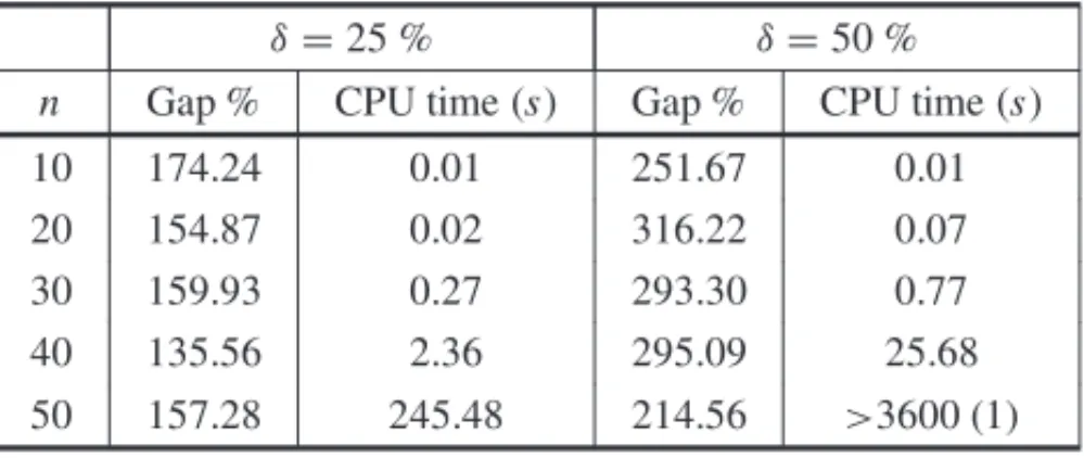
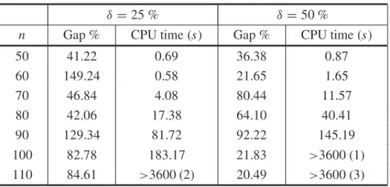
As the default preprocessing of CPLEX is able to convexify a non convex 0-1 problem, it is possible to run this state-of-the-art software without any previous reformulation of the prob-lem. Results of Tables 1 and 2 highlight how huge the duality gaps are, i.e., the gaps between the optimal continuous and integer values. For smaller densities (Table 1), all instances can be solved within one hour, except forδ =50%, where one instance cannot be solved to optimality. For larger densities (Table 2), for 40 and 50 variables, one or two instances cannot be solved exactly (see the numbers in brackets).
Table 1–Exact solutions with CPLEX 12.1 for smaller densities.
δ=25 % δ=50 %
n Gap % CPU time (s) Gap % CPU time (s)
10 174.24 0.01 251.67 0.01
20 154.87 0.02 316.22 0.07
30 159.93 0.27 293.30 0.77
40 135.56 2.36 295.09 25.68
50 157.28 245.48 214.56 >3600 (1)
2.3 A quadratic convex reformulation of the problem
perfor-Table 2–Exact solutions with CPLEX 12.1 for larger densities.
δ=75 % δ=100 %
n Gap % CPU time (s) Gap % CPU time (s)
10 255.52 0.02 321.09 0.02
20 311.45 0.23 353.79 0.58
30 306.56 9.01 725.26 21.36
40 364.78 >3600 (1) 414.04 >3600 (1) 50 752.33 >3600 (1) 726.20 >3600 (2)
mance of a state-of-the-art solver is greatly improved when it is applied after their quadratic convex reformulation called QCR, i.e., these authors observed a drastic improvement in bound quality as well as in efficiency. This is the case for the instances of our benchmark (see the re-sults of Section 2.3.2). Section 2.3.1 details before the application of the QCR method for our problem.
2.3.1 The QCR method
It consists of reformulating a nonconvex 0-1 quadratic maximization problem into an equivalent 0-1 program with a concave quadratic function. Then, the reformulated problem can be effi-ciently solved by a classical branch-and-bound algorithm based on continuous relaxation. The fundamental objective of this convexification method is therefore to construct a model whose continuous relaxation is as tight as possible.
In summary, QCR is a two-phase method, whose main phase is the preprocessing one:
• Phase 1 – Replace the objective function f(x)by a concave quadratic objective function
fα,u(x)depending on two parametersαandu both in Rn to get an equivalent convex 0-1
program (see below).
• Phase 2 –Apply a standard 0-1 convex quadratic solver to this new problem.
To be more specific, the first phase consists of perturbing the objective function by subtracting two functions, equal to zero on the feasible set and depending on two parameters.
Billionnet, Elloumi & M-C. Plateau [9] replace f(x)by:
fu,α(x)= f(x)− n
i=1
ui
x2i −xi −
n
i=1 αixi
⎛
⎝ n
j=1
xj−k ⎞
⎠ withu∈Rnandα∈Rn.
Following the results of Faye & Roupin [21], Billionnet, Elloumi & Lambert [8] propose to replace f(x)by:
fu,v(x)= f(x)− n
i=1
ui
x2i −xi −v ⎛
⎝ n
j=1
xj−k ⎞
⎠
2
The use of either of these new functions leads to identical bounds at the end of phase 1 of the QCR method. The use of the second, however, consumes the least amount of computation time. We propose thus to exploit fu,v(x)for our experiments.
The aim is thus to determine the best values of the parametersu∗ ∈Rnandv∗∈ Rso that the new function fu∗,v∗(x)is concave and the upper bound obtained by its continuous relaxation is
minimal. They are the values that optimize the following problem:
(P) min
u∈Rn, v∈R x∈[0,1]n : n max
j=1ajxj≤b, nj=1xj=k
fu,v(x)
To obtain these optimal parameters, following Billionnet et al. [8], we solve the following semi-definite relaxation of(E−k Q K P):
(E−k Q K PS D P) ⎧ ⎪ ⎪ ⎪ ⎪ ⎪ ⎪ ⎪ ⎪ ⎪ ⎪ ⎪ ⎪ ⎪ ⎪ ⎪ ⎪ ⎪ ⎪ ⎪ ⎪ ⎪ ⎪ ⎪ ⎪ ⎪ ⎨ ⎪ ⎪ ⎪ ⎪ ⎪ ⎪ ⎪ ⎪ ⎪ ⎪ ⎪ ⎪ ⎪ ⎪ ⎪ ⎪ ⎪ ⎪ ⎪ ⎪ ⎪ ⎪ ⎪ ⎪ ⎪ ⎩ max n
i=1
n
j=1
ci jXi j
s.t. Xii =xi i=1, . . . ,n (3)
n
i=1
n
j=1
Xi j−2k n
j=1
xj = −k2 (4)
n
j=1
ajxj ≤b
n
j=1
xj =k
1 xt
x X
0
x∈Rn, X ∈Rn2
where constraint(4)has been introduced to tighten the optimal value of the problem. It consists of replacing each productxixj by a variable Xi j in nj=1xj −k2 = 0 (i.e., the square of
constraint (2)).
The optimal valuesu∗i (i =1, . . . ,n)(resp.v∗) of problem(P)are simply given by the optimal values of the dual variables of(E−k Q K PS D P)associated with constraints(3)(resp.(4)).
2.3.2 Numerical experiments
large gap between results reached by CPLEX alone and CPLEX via QCR), all these experiments reinforce our purpose to elaborate dual heuristics which are able to produce within reasonable time both good lower and upper bounds for the value of problem(E−k Q K P).
Table 3–Exact solutions with CPLEX 12.1 via QCR for smaller densities.
δ=25 % δ=50 %
n Gap % CPU time (s) Gap % CPU time (s)
50 41.22 0.69 36.38 0.87
60 149.24 0.58 21.65 1.65
70 46.84 4.08 80.44 11.57
80 42.06 17.38 64.10 40.41
90 129.34 81.72 92.22 145.19
100 82.78 183.17 21.83 >3600 (1) 110 84.61 >3600 (2) 20.49 >3600 (3)
Table 4–Exact solutions with CPLEX 12.1 via QCR for larger densities.
δ=75 % δ=100 %
n Gap % CPU time (s) Gap % CPU time (s)
50 114.26 0.52 69.45 1.66
60 150.84 3.91 69.06 3.90
70 63.77 22.96 66.18 31.18
80 92.31 101.41 49.19 240.64
90 42.12 >3600 (1) 29.93 376.36 100 27.22 >3600 (4) 106.57 >3600 (2) 110 148.16 >3600 (3) 24.24 >3600 (5)
3 A PRIMAL HEURISTIC
This section presents a first lower bound for the value of problem(E −k Q K P). This basic primal heuristic, denoted byHpri, is derived from a classical heuristic devoted to the quadratic
knapsack problem [7]. As this straightforward approach exclusively provides a lower bound and consumes negligible computation times, it should be considered as a basic tool for our dual heuristics (see next Sections).
3.1 The heuristicHpr i
The primal heuristic method proposed below, denoted byHpri, is an adaptation of a well-known
• Destructive phase – A greedy algorithm derived from that of Chaillou, Hansen & Ma-hieu [15], is performed to produce a solutionxstarting from the vectore=1nofRn. This destructive procedure is simply adapted to provide a solution satisfying the capacity con-straint and with a number of items is less than or equal tok(i.e.,ax ≤bandex ≤k). This is achieved by removing iteratively itemiwith the smallest utility function of the type
j ci j
ai
.
• Constructive phase – This part performs fill up and exchange procedures. Derived from Gallo, Hammer & Simeone’s method [23], its objective is two-fold: first, to get from x a feasible solution of (E −k Q K P), that is a solution x′ satisfying the constraint capacity whose number of items placed in the knapsack is now exactly equal tok(i.e.,ax′ ≤ band
ex′=k); second, to find finally a solutionxpri which improves the quality of solutionx′.
3.2 Numerical experiments
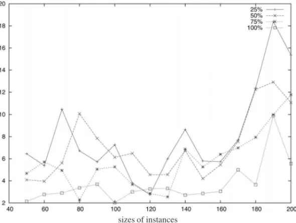
As a general remark, we note that our primal heuristicHpri is very fast, since for all instances it took less than 0.04 seconds. The duality gaps are rather small, for all instance sizes (see Fig. 2 and Table 5). The best gap values are obtained for the larger densities. Nevertheless, these gaps are markedly greater than those obtained for the classical quadratic knapsack problem, which are generally less than 1%.
4 A SEMIDEFINITE PROGRAMMING HEURISTIC
Our first effective and fast dual heuristic, denoted byHsd p, is based on semidefinite programming
(Section 4.1). Each step of this iterative procedure consists in fixing variables to zero in a solution produced by a semidefinite relaxation of the problem, before using our very fast primal heuristic over the reduced problem (Section 4.2). The computational experiments highlight the gain ob-tained by this algorithmic tool which dominates heuristics Hpri for all instances (Section 4.3).
Hsd pis very fast, since for all instances it tooks less than 4 seconds on the average.
4.1 The semidefinite programming relaxation
Let us recall [8] that from the semidefinite relaxation(E−k Q K PS D P)defined in Section 2.3.1,
we get optimal multipliersu∗∈Rnandv∗∈Rfor the QCR method such that:
v(E−k Q K PS D P)= max
x∈[0,1]n : ax≤b, ex=k fu∗,v∗(x)
We can therefore expect that problem(E−k Q K PS D P)produces good upper bounds for
/*Initial phase: provides a trivial solutionx0such thatax0≤bandex0=k*/
J←ar g k smallest(aj)j∈{1,...,n} forjfrom1tondo
ifj∈J then x0j←1 else x0j←0 endif enddo
xpri←x0;v(Hpri)← f(x0)
/*Destructive phase: provides a solutionx1such thatax1≤bandex1≤k*/
x1←e= {1, . . . ,1} U← {1, . . . ,n}
whilen
j=1aj>borcar d(U) >kdo
i∗←ar g min(
j∈Uci j/ai).
x1i∗←0 U←U− {i∗}
endwhile
ifex1=kand f(x1) > v(Hpri)then xpri←x1;v(Hpri)← f(x1)endif /*Constructive phase: fill up and exchange procedures to improvex1*/
x2←x1 bestgain←1
whilebestgaindo
bestgain←0;f illup← f alse;exchange← f alse
for allvariablexisuch thatx2i =0do if ex2<kandax2+ai≤bthen
gain←δfi /*first derivative of functionf =ci+nj=1ci jx2j*/ ifgain>bestgainthen
bestgain←gain;if ill←i,f illu p←tr ue
endif
else /*ex2=k*/
for allvariablexjsuch thatx2j=1do if ax2−aj+ai≤bthen
gain←δfi−δfj−ci j−cj i /*second derivative of functionf*/ ifgain>bestgainthen
bestgain←gain;(iex,jex)←(i,j);exchange←tr ue
endif endif endfor endif endfor
ifexchangethen
x2iex ←1;x2jex ←0 else
if f illupthenx2
if ill ←1endif endif
endwhile
ifex2=kand f(x2) > v(Hpri)then xpri←x2;v(Hpri)← f(x2)endif
sizes of instances
Figure 2–HeuristicHpri: duality gaps for each density of matrix C.
Table 5– Hsd pvs.Hpri: Gap quality. Gaps %
δ
Hpri Hsd p 25% 8.08 1.69 50% 7.09 1.67 75% 5.76 1.64 100% 3.70 1.04 Global results 6.16 1.51
Numerical experiments. Solving the semidefinite relaxation(E−k Q K PS D P)is rather fast:
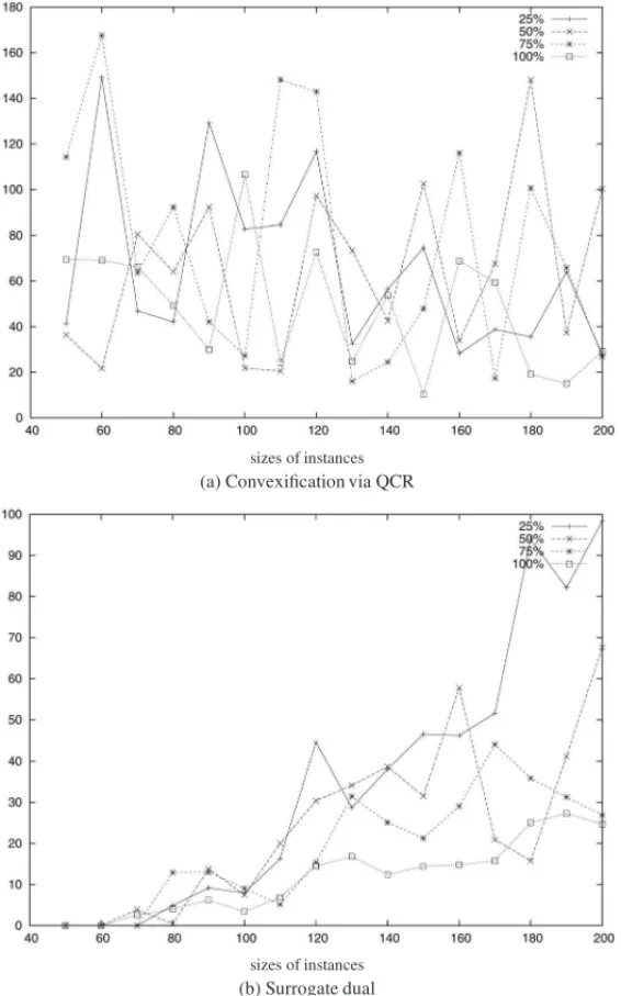
CPU times increase with the sizes of the instances without exceeding five seconds. Observing gap quality for all densities of matrix C in Figure 4 (a), the behavior of this relaxation is clearly unstable. Even if the average gap can be large (up to 150% for some instances), we still propose to use this semidefinite program for designing our heuristicHsd p.
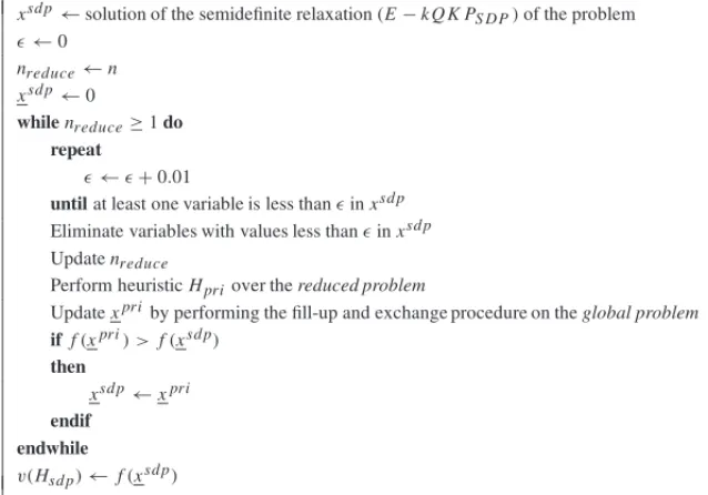
4.2 The heuristicHsd p
This heuristic method solves first the semidefinite relaxation(E−k Q K PS D P)defined in Sec-tions 2.3.1 and 4.1. Then an iterative procedure based on the associated solutionxsd pis initiated. More specifically, each step of this procedure consists in fixing more and more variables to zero inxsd p, before using our very fast primal heuristicHpri over the reduced problem. An attempt to update the solution produced by Hpri is then applied by performing the fill-up and exchange
xsd p←solution of the semidefinite relaxation(E−k Q K PS D P)of the problem
ǫ←0
nreduce←n
xsd p←0
whilenreduce≥1do repeat
ǫ←ǫ+0.01
untilat least one variable is less thanǫinxsd p
Eliminate variables with values less thanǫinxsd p
Updatenreduce
Perform heuristicHpriover thereduced problem
Updatexpriby performing the fill-up and exchange procedure on theglobal problem
if f(xpri) > f(xsd p)
then
xsd p←xpri
endif endwhile
v(Hsd p)← f(xsd p)
Figure 3–The semidefinite programming heuristicHsd p.
4.3 Numerical experiments
The performance of heuristic Hsd p is analyzed through the numerical results laid out in
Ta-bles 5, 6 and 7. Table 5 shows a great improvement regarding the quality of the duality gap. It is about three times better than that obtained byHpri. Tables 6 and 7 complete this information
by splitting the results into two categories: small sizes (n ≤ 100) and larger sizes (n ≥ 110). They reveal that CPU times remain rather low, since heuristicHsd ptooks less than 4 seconds on
the average.
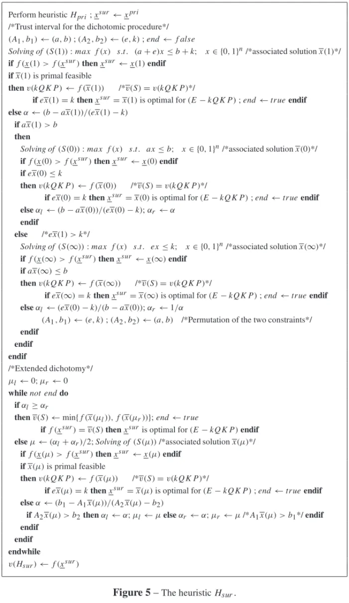
5 A SURROGATE DUAL HEURISTIC FOR(E−k Q K P)
Let us consider another effective dual heuristic, denoted by Hsur, based on a surrogate relax-ation. Eventually, this algorithmic tool will prove to be an efficient and robust method: it proves optimality for 46% of the 640 instances, within one minute on the average.
5.1 A surrogate dual algorithm
We actually use a double relaxation. We first consider the following problem for which the equality cardinality constraint(2)is transformed into an inequality constraint(2′):
(k Q K P)
⎧ ⎪ ⎪ ⎪ ⎪ ⎨
⎪ ⎪ ⎪ ⎪ ⎩
max f(x)
s.t. ax ≤b (1)
ex ≤k (2′)
Second, we consider a surrogate relaxation of this 0-1 quadratic bi-knapsack problem, by com-bining the two constraints(1)and(2′). To solve the associated surrogate dual problem, we use the scheme of the algorithmS AD E2developed by Fr´eville & G. Plateau [22] for the surrogate dual oflinear0-1 bi-dimensional knapsack problems.S AD E2is a one-dimensional dichotomic search over the compact interval [0,1], which revisits Glover’s method [24] for guaranteeing optimality in a finite number of iterations.
In short, given a multiplierµ∈ [0,1], algorithmS AD E2determines first an order on the two constraints (1) and (2’), so that the surrogate relaxation can be written as:
(S(µ))
⎧ ⎪ ⎨
⎪ ⎩
max f(x)
s.t. (A1+µA2)x ≤(b1+µb2)
x ∈ {0,1}n
with either
(A1,b1)=(a,b) and (A2,b2)=(e,k)
or
(A1,b1)=(e,k) and (A2,b2)=(a,b)
For a givenµ, letx∗(µ)be an optimal solution of problem(S(µ)), ifx∗(µ)satisfies simultane-ously the two constraints, it is obvisimultane-ously an optimal solution of problem(k Q K P). If, in addition,
ax∗(µ) =k, the problem(E−k Q K P)is solved. Otherwise, procedureS AD E2performs its dichotomic search by using the fact thatx∗(µ)satisfies the first (resp. second) constraint and violates the second (resp. first) one, and by exploiting the ratio(b1−A1x∗(µ))/(A2x∗(µ)−b2) to update the interval bounds (see [22]).
As the theoretical results for this method depend only on properties of the bi-constraint system, its adaptation for the quadratic case is straightforward. In addition, at each iteration of the procedure, we propose to exploit the approach of Caprara, Pisinger & Toth [14] for solving the associated quadratic 0-1 knapsack instance (this requires to adapt their code for accepting a constraint with real data). The first step of Caprara et al.’s method consists of linearizing(S(µ))as follows:
⎧ ⎪ ⎪ ⎪ ⎪ ⎪ ⎪ ⎪ ⎪ ⎪ ⎪ ⎪ ⎪ ⎪ ⎪ ⎪ ⎨ ⎪ ⎪ ⎪ ⎪ ⎪ ⎪ ⎪ ⎪ ⎪ ⎪ ⎪ ⎪ ⎪ ⎪ ⎪ ⎩
max f(x,y)= j∈N
cj jxj + j∈N
i∈N\{j} ci jyi j
s.t.
j∈N
(a1j+µa2j)xj ≤b1+µb2
i∈N\{j}
(a1i+µa2i)yi j ≤(b1+µb2−(a1j+µa2j))xj ∀j ∈ N (5)
0≤yi j ≤xj ≤1 ∀(i,j)∈N2,i= j
yi j =yj i ∀(i,j)∈N2,i < j (6)
xi,yi j ∈ {0,1} ∀(i,j)∈ N2,i = j
to the old one by suitable inequalities. Indeed, constraints(5)result from multiplying the capac-ity constraint by each variable and replacingx2j byxj since the variables are binary variables.
They are redundant as long as the integer restriction on the variables is imposed. Caprara et al. solve this problem by a branch-and-bound method based on a depth-first search strategy with a static order of the variables for branching. It uses a preprocessing phase which reduces the size of the problem through variable fixing. Its effectiveness is obtained by algorithmic choices and data structures that favor simplicity and incrementality (as for the algorithm designed for the linear 0-1 knapsack problem in [33]). In particular, their evaluation of nodes is based on a Lagrangian relaxation of(L P(µ)) which dualizes the symmetric constraints (6). The authors highlight a beautiful decomposition result which shows that solving this relaxation is equivalent to solven+1 linear 0-1 knapsack problems. Furthermore, for controling time complexity, the authors decide to relax the integer conditions on variables. This leads to an evaluation which can be produced in 0(n2)time since each continuous linear knapsack problem can be solved in 0(n)time [20].
From a practical point of view, in order to control CPU times (i.e., to speed up achieving good upper bound for v(k Q K P) and thus for v(E −k Q K P)), we propose to search an approxi-mate value of the surrogate dual(S)of(k Q K P)by means of the following two algorithmic adaptations:
– approximation 1 (solving problem(S(µ))):
We add a CPU time limit (one minute, in our case) in the branch-and-bound search of Caprara et al.’s method. Obviously, this stopping criterion is effective when the Lagrangian relaxation evaluation is inefficient. In practice, this occurs for values ofµclose to zero, or for the greater instance sizes (around 200 variables). In this situation, we have retained first the upper bound vup(S(µ))on the value of(S(µ)), equal to the maximal evaluation over the pending nodes of the search tree, and also the associated solutionxup(µ)of(S(µ)).
– approximation 2 (in the dichotomic search):
The performance of Caprara et al.’s method is poor for a problem like(S(0)), whose constraint coefficients are all identical (equal to one here). When no solution is found by Caprara et al.’s method within the CPU time limit, we propose to increase multiplierµstep by step from zero (i.e., we start with value 0.01, then double that value each time). This process stops as soon as a multiplierµt is found such that problem(S(µt))can be solved to optimality within the CPU time limit.
Whileapproximation 2implies that the set Mof multipliers generated by our approximate dual algorithm may miss the optimal multiplierµ∗for(S), withapproximation 1, we can conclude that our dual algorithm finds an upper boundv(S)ofv(S)defined as follows:
v(S)=min
µ∈Mv(S(µ))
Proposition.
v(E−k Q K P)≤ v(k Q K P)≤ v(S)= min
µ∈[0,1]v(S(µ))≤ v(S)=µ∈minMv(S(µ))
Finally, in the algorithm of Figure 5, for anyµ,solving(S(µ))may besolve(S(µ)) approxi-matelywhenapproximation 1occurs. In this case, we exploit the solutionxup(µ)(see above) that may differ fromx∗(µ). All along our approximate dual method, we propose to denote this solution byx(µ), which is equal toxup(µ)ifapproximation 1is being used, orx∗(µ)otherwise.
sizes of instances (a) Convexification via QCR
sizes of instances (b) Surrogate dual
Numerical experiments. As for the linear case, our approximate surrogate dual value is reached in a finite number of iterations (at most 10 iterations here). From the results obtained with this dichotomic procedure, two global remarks may be mentioned: first, CPU times do not exceed seven minutes on the average and above all the quality of upper bounds is very good (see Fig. 4(b)). Second, more than 75% of gap values are improved in comparison with those produced by the semidefinite programming relaxation (see Section 4).
5.2 The surrogate dual heuristicHsur
Classically, our surrogate dual heuristic, denoted by Hsur, keeps the best feasible solution of
(E −k Q K P), denoted byxsur, produced by the dichotomic procedure described in Figure 5. It computes both a lower bound f(xsur)and an upper boundv(S)(see Section 5.1) ofv(E−
k Q K P).
More specifically, at each iteration of our dichotomic procedure, that is for each multiplierµin the set M defined above, we retain the best feasible solution – denoted byx(µ)– produced by the branch-and-bound depth first search, which satisfies the cardinality constraint exactly (i.e.,
ax(µ)≤bandex(µ)=k).
As the procedure starts by using the very fast heuristicHpri, the solutionxsur produced by our
heuristicHsur is such that:
fxsur=maxf(xpri),max
µ∈M f(x(µ))
Using an analysis of the experimental results of the previous section, the single adjustment of our procedure consists in reducing to half a minute the CPU time threshold for solving(S(µ)) approximately (its solution is denoted byx(µ)(see Section 5.1)). This allows first, to speed up the search with a negligible loss in gap quality and second, to get a dual heuristic which is both effective and robust. Finally, it should be noted that problem(E −k Q K P)is solved exactly when a problemS(µ)is solved exactly for a givenµinM and when its optimal solutionx(µ)is primal feasible for(E−k Q K P)(see Proposition of Section 5.1).
Numerical experiments. The numerical results of Figure 6 (associated with those of Table 6 and Table 7) show the high quality of the lower bounds provided by our surrogate dual heuristic
Hsur. It tends to dominate heuristicHsd pon the instances of small sizes (n ≤ 100), while the reverse is true for the larger sizes (n≥110). It should be noted that 46% of the instances are in fact exactly solved by our surrogate dual heuristic. Although CPU times ofHsur increase with
the size of the instances, they never exceed two minutes. Moreover, for each density, the mean time is around one minute.
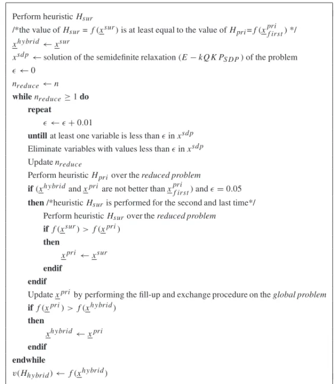
6 A HYBRID DUAL HEURISTIC
Our fast and efficient hybrid heuristic method, denoted byHh ybrid, combines the heuristics
Perform heuristicHpri;xsur←xpri /*Trust interval for the dichotomic procedure*/ (A1,b1)←(a,b);(A2,b2)←(e,k);end← f alse
Solving of(S(1)):max f(x) s.t. (a+e)x≤b+k; x∈ {0,1}n/*associated solutionx(1)*/
iff(x(1) > f(xsur)thenxsur←x(1)endif ifx(1)is primal feasible
thenv(k Q K P)← f(x(1)) /*v(S)=v(k Q K P)*/
ifex(1)=kthenxsur=x(1)is optimal for(E−k Q K P);end←tr ueendif elseα←(b−ax(1))/(ex(1)−k)
ifax(1) >b
then
Solving of(S(0)):max f(x) s.t. ax≤b; x∈ {0,1}n/*associated solutionx(0)*/
if f(x(0) > f(xsur)thenxsur←x(0)endif ifex(0)≤k
thenv(k Q K P)← f(x(0)) /*v(S)=v(k Q K P)*/
ifex(0)=kthenxsur=x(0)is optimal for(E−k Q K P);end←tr ueendif elseαl←(b−ax(0))/(ex(0)−k);αr←α
endif
else /*ex(1) >k*/
Solving of(S(∞)):max f(x) s.t. ex≤k; x∈ {0,1}n/*associated solutionx(∞)*/
if f(x(∞) > f(xsur)thenxsur←x(∞)endif ifax(∞)≤b
thenv(k Q K P)← f(x(∞)) /*v(S)=v(k Q K P)*/
ifex(∞)=kthenxsur =x(∞)is optimal for(E−k Q K P);end←tr ueendif elseαl←(ex(0)−k)/(b−ax(0));αr←1/α
(A1,b1)←(e,k);(A2,b2)←(a,b) /*Permutation of the two constraints*/
endif endif endif
/*Extended dichotomy*/ µl←0;µr←0 whilenot enddo
ifαl≥αr
thenv(S)←min{f(x(µl)),f(x(µr))};end←tr ue
if f(xsur)=v(S)thenxsuris optimal for(E−k Q K P)endif elseµ←(αl+αr)/2;Solving of(S(µ))/*associated solutionx(µ)*/
if f(x(µ) > f(xsur)thenxsur←x(µ)endif ifx(µ)is primal feasible
thenv(k Q K P)← f(x(µ)) /*v(S)=v(k Q K P)*/
ifex(µ)=kthenxsur =x(µ)is optimal for(E−k Q K P);end←tr ueendif elseα←(b1−A1x(µ))/(A2x(µ)−b2)
ifA2x(µ) >b2thenαl←α;µl←µelseαr←α;µr←µ/*A1x(µ) >b1*/endif
endif endif endwhile
v(Hsur)← f(xsur)
sizes of instances (a) Duality gaps
sizes of instances (b) CPU times (s)
Figure 6–HeuristicHsur(results for each density of matrix C).
within the semidefinite programming reduction phase. It proves to get best duality gaps in a reasonable time for all instances of our benchmark.
6.1 The heuristicHh y br i d
The aim of this heuristic (see Fig. 7) is to get better solutions than those provided by our heuristics
apply heuristicHsd p(see Fig. 3) in which heuristicHsur is used for a second and last time. We
are thefore sure to find a solutionxh ybrid as good as that produced by both heuristicsHpri,Hsd p
and Hsur. In addition, computation times remain reasonable since heuristicHsur is used only
two times. They are in addition to the reasonable time ofHsd p.
Perform heuristicHsur
/*the value ofHsur=f(xsur)is at least equal to the value ofHpri=f(xprif irst)*/
xh ybrid←xsur
xsd p←solution of the semidefinite relaxation(E−k Q K PS D P)of the problem
ǫ←0
nreduce←n whilenreduce≥1do
repeat
ǫ←ǫ+0.01
untillat least one variable is less thanǫinxsd p
Eliminate variables with values less thanǫinxsd p
Updatenreduce
Perform heuristicHpriover thereduced problem
if(xh ybridandxpriare not better thanxprif irst)andǫ=0.05
then/*heuristicHsuris performed for the second and last time*/ Perform heuristicHsurover thereduced problem
if f(xsur) > f(xpri)
then
xpri←xsur
endif endif
Updatexpriby performing the fill-up and exchange procedure on theglobal problem
if f(xpri) > f(xh ybrid)
then
xh ybrid←xpri
endif endwhile
v(Hh ybrid)← f(xh ybrid)
Figure 7–The heuristicHh ybrid.
6.2 Numerical experiments
The computational experiments validate the relevance of the bounds produced by our hybrid heuristic method which combines quality (i.e., duality gap is about 1.20 % on the average) and efficiency (i.e., CPU time is about one minute and a half on the average).
sizes of instances (a) Duality gaps
sizes of instances (b) CPU times (s)
Figure 8–HeuristicHh ybrid(results for each density of matrix C).
software, denoted byL T−C P L E X, are listed in Tables 6 and 7. Figure 9(a) (duality gaps) show clearly, instance size by instance size, the dominance ofHh ybrid overHsur andL T −C P L E X.
sizes of instances (a) Duality gaps (%)
sizes of instances (b) CPU time (s)
Figure 9– Hh ybrid vs.Hsurandli mi ted ti me C P L E X.
For the set of 550 instances (resp. 640 instances), heuristicHh ybrid yields thus known optima in
90% (resp. 76%) of the cases and proves optimality in 63% (resp. 49%) of the cases, within less than 100 seconds on the average. These scores are even better for instances with sizes from 50 to 100 variables. For example, Hh ybrid yields known optima in 96% of the cases (i.e., 232 of 240
instances).
Table 6–Hh ybridvs.Hsd p,Hsur andL T−C P L E X: average values forn=50 to 100. HeuristicHsd p HeuristicHsur HeuristicHh ybrid L T −C P L E X
δ Gap % CPU (s) Gap % CPU (s) Gap % CPU (s) Gap %
25 % 0.60 1.55 0.22 19.15 0.01 26.14 1.62
50 % 0.43 1.70 0.80 32.28 0.03 44.64 2.11
75 % 0.22 1.46 0.20 27.27 0.03 37.71 2.28
100 % 0.35 1.51 0.27 18.55 0.03 28.43 1.27
Global results 0.40 1.56 0.37 25.06 0.03 34.23 1.82
Table 7– Hh ybrid vs.Hsd p,Hsur andL T−C P L E X: average values forn=110 to 200. HeuristicHsd p HeuristicHsur HeuristicHh ybrid L T−C P L E X
δ Gap % CPU (s) Gap % CPU (s) Gap % CPU (s) Gap %
25 % 2.42 6.91 4.95 68.10 1.98 111.11 3.99
50 % 2.41 6.12 3.57 80.16 2.03 128.87 4.41
75 % 2.51 6.14 3.43 80.36 2.19 130.05 4.15
100 % 1.45 6.66 2.47 75.17 1.30 132.19 2.65
Global 2.20 6.46 3.61 75.95 1.88 125.56 3.80
Table 8–HeuristicHh ybrid: performance for all sizes. Optimality
δ Gap % CPU (s) Proved % Reached % 25 % 1.25 79.25 47.95 (58.82) 80.14 (92.13) 50 % 1.28 97.28 51.33 (65.25) 77.33 (89.92) 75 % 1.38 95.43 47.02 (61.74) 72.85 (88.00) 100 % 0.82 93.28 51.32 (66.67) 74.34 (88.28) Global 1.18 91.31 49.42 (63.11) 76.13 (89.59)
7 CONCLUSION
ACKNOWLEDGEMENTS
This work was partially conducted on the Magi cluster at Universit´e Paris 13, and available at
http://www.univ-paris13.fr/calcul/wiki/.
REFERENCES
[1] ADAMS WP, FORRESTER R & GLOVERF. 2004. Comparisons and enhance ment strategies for linearizing mixed 0-1 quadratic programs.Discrete Optimization,1(2): 99–120.
[2] AHLATI¸OGLUA & GUIGNARDM. 2007. The convex hull relaxation for nonlinear programs with linear constraints. Technical report, OPIM Department, Wharton School (USA).
[3] BALASE & ZEMELE. 1980. An algorithm for large zero-one knapsack problems.Operations Re-search,28: 1130–1154.
[4] BERTSIMASD & SHIODAR. 2009. Algorithm for cardinality-constrained quadratic optimization.
Computational Optimization and Applications,43: 1–22.
[5] BIENSTOCKD. 1996. Computational study of a family of mixed-integer quadratic programming problems.Mathematical Programming,74: 121–140.
[6] BILLIONNETA. 2005. Different formulations for solving the heaviestk-subgraph problem. Informa-tion Systems and OperaInforma-tional Research,43(3): 171–186.
[7] BILLIONNETA & CALMELSD. 1996. Linear programming for the 0-1 quadratic knapsack problem.
European Journal of Operational Research,92: 310–325.
[8] BILLIONNETA, ELLOUMIS & LAMBERTA. Extending the QCR method to general mixed-integer programs. Mathematical Programming, Pub. on line, 21 pages, Doi: 10.1007/s10107-010-0381-7. [9] BILLIONNETA, ELLOUMI S & PLATEAUM-C. 2009. Improving the performance of standard
solvers via a tighter convex reformulation of constrained quadratic 0-1 programs: the QCR method.
Discrete Applied Mathematics,157: 1185–1197.
[10] BONAMIP & LEJEUNEM. 2009. An exact solution approach for portfolio optimization problems under stochastic and integer constraints.Operations Research,57: 650–670.
[11] BORCHERSS. 1999. CSDP, a C library for semidefinite programming.Optimization methods and Software,11(1): 613–623.
[12] BOROSE & HAMMERP. 2002. Pseudo-boolean optimization.Discrete Applied Mathematics,123: 115–225.
[13] CAPRARAA, KELLERERH, PFERSCHYU & PISINGERD. 2000. Approximate algorithms for knap-sack problems with cardinality constraints.European Journal of Operational Research,123: 333– 345.
[14] CAPRARAA, PISINGERD & TOTH P. 1999. Exact solution of the quadratic knapsack problem.
INFORMS Journal on Computing, 11: 125–137.
[15] CHAILLOUP, HANSENP & MAHIEUY. 1986. Best network flow bounds for the quadratic knapsack problem.Lecture Notes in Mathematics,1403: 226–235.
[17] COIN-OR. COmputational INfrastructure for Operations Research.http://www.coin-or. org.
[18] CPLEX. 2009. IBM ILOG CPLEX Callable library version 12.1 Reference manual. http:// docs.hpc.maths.unsw.edu.au/ilog/cplex/12.1.
[19] DUDZINSKIK. 1989. On a cardinality constrained linear programming knapsack problem. Opera-tions Research Letters,8: 215–218.
[20] FAYARDD & PLATEAUG. 1982. Algorithm 47: an algorithm for the solution of the 0-1 knapsack problem.Computing,28: 269–287.
[21] FAYEA & ROUPINF. 2007. Partial Lagrangian relaxation for general quadratic programming.4OR, 5(1): 75–88.
[22] FREVILLE´ A & PLATEAUG. 1993. An exact search for the solution of the surrogate dual of the 0-1 bidimensional knapsack problem.European Journal of Operational Research,68: 413–421. [23] GALLOG, HAMMERPL & SIMEONEB. 1980. Quadratic knapsack problems.Mathematical
Pro-gramming Study,12: 132–149.
[24] GLOVERF. 1965. A multiphase dual algorithm for the 0-1 integer programming problem.Operations Research,13(6): 879–919.
[25] HAMMERP, HANSENP & SIMEONEB. 1984. Roof duality, Complementation and Persistency in Quadratic 0-1 Optimization.Mathematical Programming,28: 121–155.
[26] HELMBERGC & RENDLF. 1998. Solving quadratic (0,1)-problems by semidefinite programs and cutting planes.Mathematical Programming,8(3): 291–315.
[27] HELMBERG C, RENDL F & WEISMANTEL R. 2000. A semidefinite programming approach to quadratic knapsack problems.Journal of Combinatorial Optimization,4: 197–215.
[28] KELLERERH, PFERSCHYU & PISINGERD. 2004. Knapsack Problems. Springer-Verlag.
[29] L ´ETOCARTL, PLATEAUMC & PLATEAUG. 2007. Lagrangean and convexification methods for the 0-1k-item quadratic knapsack problem. In Proceedings of NCP07 (International Conference on Non Convex Programming), Rouen (France), December.
[30] MICHELONP & MACULANN. 1991. Lagrangean decomposition for integer nonlinear programming with linear constraints.Mathematical Programming,52(2): 303–314.
[31] MITRA G, ELLISONF & SCOWCROFTA. 2007. Quadratic programming for portfolio planning: Insights into algorithmic and computational issues. Part ii: Processing of portfolio planning models with discrete constraints.Journal of Asset Management,8: 249–258.
[32] PISINGERD. 2007. The quadratic knapsack problem: a survey.Discrete Applied Mathematics,155: 623–648.
[33] PLATEAUG & NAGIHA. 2010. 0-1 Knapsack Problems. In Combinatorial Optimization: Paradigms of Combinatorial Optimization (V. Paschos eds), ISTE ltd-John WILEY and Sons Pub., volume 2, chapter 8, 215–242.
[34] POSNERME & GUIGNARDM. 1978. The collapsing 0-1 knapsack problem.Mathematical Pro-gramming,15: 155–161.
[36] SHERALIHD & ADAMSWP. 1999. A Reformulation-Linearization Tech nique for Solving Discrete and Continuous Nonconvex Problems. Kluwer Academic Publ., Dordrecht, Boston, London. [37] ZHUWX. 2003. Penalty parameter for linearly constrained 0-1 quadratic programming.Journal of