J. of the Braz. Soc. of Mech. Sci. & Eng. Copyright 2006 by ABCM October-December 2006, Vol. XXVIII, No. 4 /467
Giovanni M. Gouveia
Didier Lemosse
Emmanuel Pagnacco
Eduardo S. de Cursi
[email protected] LMR, INSA de Rouen BP 08 Av de l’Université Saint Etienne du Rouvray. France
Franck Dujardin
[email protected] CHU Rouen 1 r Germont 76000 Rouen. France
Dedicated Procedures for Temporal
Identification in a Flexible Multi-body
System
The aim of this paper is to evaluate forces and torques in flexible joints of a flexible multi-body system (FMS). To represent such a FMS a 2D non-linear model based on finite element method is built. Its numerical form solution based on a stable integration scheme and on the non-linear Newton-Raphson method is described. As the evaluation procedure first requires that some model physical properties are obtained as identified parameters, two procedures are used: direct and indirect identification. They are respectively based on dynamic equilibrium verification and on comparison between simulated and measured kinematics of the proposed model. The development of the two procedures and a performance comparison between them is carried out.
Keywords: Temporal identification, flexible multi-body system, dynamic simulation
Introduction
Many studies have shown that some kinematics and dynamic factors play an important role in osteoarthritis of hip joint (Dujardin et al, 1997), (Mejjad et al, 1998). A better comprehension of this disease evolution, it's related causes as well as a better understanding of worn phenomenon of femur implant, is needed. Thus the evaluation of the dynamic efforts arising in the contact between the head of the femur and the hip in a normal human activity are necessary. Nevertheless the use of inner sensors would be extremely hard to implement, not to mention the troublesome for the user.1
Then, the remained option is to evaluate those efforts by means of a mathematical model. Models classically used in biomechanical studies are based on the rigid body motion hypothesis. These last are neither reliable nor ranged in terms of uncertainties in the case of dynamic flexible systems. Nevertheless, with such rigid behavior, mechanical parameters can be evaluated directly through an inverse dynamic strategy. The method consists in introducing measured kinematics in the equilibrium dynamic equations and considering external load and other parameters as unknowns. This can be quite easily done because few kinematics parameters are necessary. The whole kinematics behavior of a rigid solid can be described by only six parameters: 3 displacements and 3 rotations. A similar approach, called direct identification procedure, may be followed in the case of flexible models. However, the method needs that all kinematics data during a human gait are obtained, what is a challenge. One has to notice that in the case of flexible bodies a continuous field describes the whole kinematics. That means that a large number of parameters are necessary to identify each body configuration that
Presented at XI DINAME – International Symposium on Dynamic Problems of Mechanics, February 28th - March 4th, 2005, Ouro Preto. MG. Brazil. Paper accepted: June, 2005. Technical Editors: J.R.F. Arruda and D.A. Rade.
implies in a measure system able to capture the whole body kinematics. An adapted identification and an indirect identification procedure dealing with only a part of the kinematics data are proposed in order to answer this need.
These three different procedures are described in the following sections. A comparison, between direct and indirect, will be made later through a numerical study involving a non-linear model based on the concept of open-chain mechanisms with flexible beams and imperfect joints in 2D space. The adapted direct procedure will be analyzed separately. Those procedures shall be able to evaluate some physical parameters of that model and have in common a main development axis which consists in the two following steps:
- Write the differential algebraic equations DAE of the dynamic flexible system by Eq. (1) employing some supposed known parameters psol and using Finite Element approach (Terms in Eq. (1) will be explained in the next section).
( )
( )
( )
= = − − + + +
0 q
Φ
0 g f
λ
B f q M q
Mɺɺt ɺɺt int T ext
(1)
- Solve them by using a temporal resolution scheme that will allow to gather the data set or reference kinematics set of the problem. This reference kinematics set is composed of positions, velocities and accelerations of nodal variables. A bar placed over the variables in following sections will represent reference set.
Nomenclature
q = kinematics degrees of freedom M = complete mass matrix f = generalized force vector
Φ Φ Φ
Φ= constraint equations λλλλ = Lagrange coefficient
R = rotation operator
r = residue vector of dynamic equilibrium
rΦΦΦΦ = residue vector of constraint equations
Greek Symbols
α = damping coefficient c = partial derivative ∆ = increment
Subscripts & Superscript
int = internal terms ext = external terms T = transpose i = relative to element t = studied time ∆t = time increment n = iteration number
Remarks about the Development of DAE
To evaluate all terms of the dynamic and constraint equations of DAE, we need many structural data as geometric and material information of the problem. We also need the involved external forces. All those data can be regarded as a parameter set p. The development of DAE is made for the two basic elements employed in the problem: the co-rotational beam and the co-rotational linear and torsional spring. We also need to develop their stiffness elemental matrix as preparatory step to the solution of DAE.
It has been chosen to write the equilibrium equations using as kinematics degrees of freedom the positions of nodes. These positions are collected in a single vector q. The inertia Mqɺɺ and gyroscopic Mqɺ ɺ forces in Eq. (1) are evaluated from kinetic energy of a constant section beam. The complete mass matrix M, related to inertia forces, can be obtained by assembling of the element mass matrix Mi, which can be found in (Dhatt and Batoz, 1990) in their corresponded degrees of freedom. The elementary mass matrix Mi
corresponding to spring element is set to null matrix due to hypothesis of its absence of mass. The mass temporal derivative
ɺ
M, related to gyroscopic forces, is obtained from a similar way with its elemental matrix Mɺi given by Eq. (2). R is the rotation operator describing the orientation of the element with respect to an inertial frame. i i T i i i T i
i R M R R M R
Mɺ = ɺ + ɺ (2)
The evaluation of internal forces fint of beams and linear springs is made through a co-rotational element formulation using Kirchhoff theory described in (Crisfield, 1991). The aim of this formulation is to subtract the rigid displacements, translation and rotation, from the total displacement of an element. This operation allows us to keep only elastic displacements and to compare them to the undeformed element. After that, one can assign this filtered deformation to the developed internal forces and torques. The evaluation of internal forces fint concerning the torsional spring element is straightforward because they are not under influence of the rigid displacements of the element.
The term B λ
T
represents the reaction forces, i.e. the developed efforts to satisfy the constraint equations of the second part of Eq. (1). The vector ΦΦΦΦ represents all system constraint equations. These last are written as functions of our predefined global nodal variables q.
Thus, B represents the gradient of ΦΦ vector related to ΦΦ q. The vector λ λ quantifies the influence of each constraint in the system λ λ forces. It is obtained during the temporal resolution as additional variables.
The two last terms of Eq. (1) are the external forces fext and the field force g. Each nodal external force applied in the dynamic system must be placed in its corresponding degree of freedom in the global vector fext. The vector g is built from the assembly of elemental field forces also in its degree of freedom. This elemental field force is defined as being the derivative of the elemental potential energy with respect to adopted co-ordinates q. The elemental field forces corresponding to co-rotational linear and torsional spring are set to null vector due to their absence of mass, as stated before.
Temporal Resolution Scheme of DAE
Finding the solution of Eq. (1) in time t+∆t implies to find a variable set
(
t+∆t t+∆t t+∆t t+∆t)
λ
q q
qɺ ,ɺ , ,
ɺ that verifies its two equations simultaneously. Near of the solution, the vectors
(
t+∆t t+∆t t+∆t t+∆t)
λ
q q q
rɺɺ ,ɺ , , and rΦ
(
qt+∆t)
, defined in Eq. (3)must tend to 0.
( )
qΦ r g f λ B f q M q M r Φ = − − + + + = ext T int ɺ ɺ ɺ ɺ (3)
However, the presence of constraint equations in DAE can cause severe instabilities in DAE responses. The importance of high frequencies in those responses is reduced in order to avoid those instabilities. This is done by the evaluation of the residual vectors through Eq. (4) and Eq. (5). That means that between two very close times, t and t+∆t, the acceleration is supposed constant.
(
)
(
(
)
)
( )
(
)
( )
αext t t T t t t t t t t t T t t t t t t t t t t t t t α α f g λ B q f q M g λ B q f q M q M r − − + + − − + + + + = ∆ + ∆ + ∆ + ∆ + ∆ + ∆ + ∆ + ∆ + int int 1 ɺ ɺ ɺ ɺ ɺ ɺ (4)
(
t t t) (
α) (
t t)
α( )
qtΦ
q
Φ
q q
rΦ = + −
∆ + ∆
+ , 1 (5)
( )(
)
α t✍
t t
α
tα = 1+ + − is a time between t and t+∆t. This
procedure, named Hilber-Hughes-Taylor (HHT) (Jalon and Bayo, 1994), imposes less loss of total energy during the numerical resolution procedure than a stabilized Newmark method. The strategy starts from a known equilibrium set
(
t t t t)
λ
q q
qɺɺ,ɺ , , at the time t. A perturbation is then imposed to this variable in order to have a prediction of the equilibrium state at time t+∆t by using Eq. (6).
(
)
( )
t t t t t t t t t t t t t t t ✏ t γ ✏ t β ✏ t λ λ q q q q q q q q q = = − + = − + + = ∆ + ∆ + ∆ + ∆ + 0 0 0 2 0 1 2 / 1 ɺ ɺ ɺ ɺ ɺ ɺ ɺ ɺ ɺ ɺ ɺ (6)with α
γ = −
2 /
1 and
( )
1 α 2/4β
−
= . The stability parameters γ and β are related to a numeric dumping parameter α . It can be
J. of the Braz. Soc. of Mech. Sci. & Eng. Copyright 2006 by ABCM October-December 2006, Vol. XXVIII, No. 4 /469 unconditionally stable and second-order accurate in the absence of
constraint (Geradin and Cardona, 2000). α =0
meaning that no numeric damping is added to the solution to avoid numerical instabilities, corresponding to classical Newmark scheme. In the other hand, α 1/3
−
= means a great numeric dumping and brings to the system solution a high loss of energy.
Non Linear Solution
The DAE we deal with is a non-linear system of equations and imposes to solve an adapted procedure. The tangent matrix of the system has to be evaluated because the classical Newton-Raphson (NR) method has been chosen. It is given by the differential of the residual vector with respect to q as shown in Eq. (7).
(
)
✂t t T ext
T =∂∂ + − + − + +
λ B f f g M M q
K ɺ int (7)
The term concerning the internal forces is the only one having to be evaluated and can be found in (Crisfield, 1991). The differential with respect to q of the two first terms of Eq. (7) are very costly to evaluate just for convergence (Geradin and Cardona, 2000). The remaining terms are constant with respect to q, Equation (1) has to be linearized in Eq. (8) form in order to apply the classical NR method.
(
)
( )
− = − = + + + + + + + + n☎ t t n n☎ t t n☎ t t n☎ t t n☎ t t T n n T n n ✆ , , , ✆ ✆ ✆ ✆ q r q B λ q q q r λ B q K q M q M Φ ɺ ɺ ɺ ɺ ɺ ɺ ɺ (8)The exponent n being the iteration number. With the chosen temporal integration scheme, Eq. (8) can be rewritten in matrix form of Eq. (9). This equation corresponds to a linear system.
− = Φ r r λ q 0 B B S ✡ ✡ T
T with
T
T β ☞
t γ β ☞ t K M M
S = + ɺ +
2 (9)
Variables are updated during the NR process by means of Eq. (10). λ λ λ q q q q q q q q q ✎ ✎ β ✎ t γ ✎ β ✎ t ✎ n✒ t t n✒ t t n✒ t t n✒ t t n✒ t t n✒ t t n✒ t t n✒ t t + = + = + = + = + + + + + + + + + + + + 1 1 1 2 1 / / ɺ ɺ ɺ ɺ ɺ ɺ (10)
The process stops when the convergence of the residual vectors, Eq. (4) and Eq (5) evaluated by the HHT scheme, is checked.
Direct Temporal Identification
The direct strategy is based on the dynamic equilibrium equation Eq. (1). If a complete set of variable kinematics response
(
ɺqɺt,qɺt,qt)
and a set of parameters(
t)
λ
p, of a dynamic system are available, the residual equilibrium
(
t)
λ
p
z , of those parameter can be evaluated at time t by Eq. (11).
(
)
( )
( )
+ + + − − = = Φ g f λ B f q M q M p Φ r λ p r λ p z ext T t t , int , ɺ ɺ ɺ ɺ (11)with M
(
p,qt)
, Mɺ(
p,qt,qɺt)
and fint(
p,qt)
being functions of parameters p and of measured data qt and qɺt. The constraint equation Φ(
pqt)
, is function of parameters p and of unknown data
t
q . The set of parameters
( )
*,λ *tp that is solution gives a residue null or at least minimize it with experimental data. Then, the proposed solution can be regarded as an optimization procedure declared by means of Eq. (12) searching for a parameter set
( )
*,λ *tp
minimizing residues of Eq. (11).
( )
λ Argmin( )(
z z)
p λ p T t J t = = , * * , (12)
At any studied time t, this z residual vector, which is non linear dependent from p and λλλλt, has to be equalized to zero. This can be done by a classical less squares method and a first order
Newton-Raphson strategy. Starting from a given
( )
0,λ 0tp , parameters are interactively modified through Eq. (13) until convergence is reached. z p z λ p λ p + ∂ ∂ − = + + n t n n t n 1 1 (13)
In that expression,
(
∂z/∂p)
+ is called (Moore-Penrose) pseudo-inverse matrix of residual gradient matrix ∂z/∂p. It is numerically evaluated by a central finite difference procedure.This strategy is numerically efficient because it is based on an interactive procedure. Especially, no temporal resolution is needed. Nevertheless, it shows a high sensibility to introduced measures and especially to accelerations.
The main difficulty stays in the need of having measured data for all degrees of freedom introduced in the model. If this can be hardly done for displacement variables, it is almost impossible for rotation variables, much less in the context of bio-mechanic study in which humans have to be instrumented. In order to avoid this difficulty an indirect procedure using only available kinematics variables have been proposed.
Adapted Direct Temporal Identification
This proposed procedure consists in using only linear displacement variables and their first and second time derivatives as measured data of the dynamic problem. The remained variables, i.e. the rotation variables, their first and second time derivatives, the Lagrange parameters as well as other physic and geometric structural parameters such as stiffness are treated as the parameters to be identified.
only the time t+∆t has been used. The task becomes easier if continuous variables through a temporal polynomial approximation replace discrete ones. Then, rotations have the following expression presented in Eq. 14.
( ) ( )
( )
( )
34 2 3 2
1i c it c it c it
c
i= + + +
θ (14)
The terms cj
( )
i being constants and the term i corresponding tothe node number of the dynamic structure. The first and second derivative of θi are then obtained by deriving those expressions with
respect to t. The total number of unknown parameters describing the rotation in a node around the time t is here fixed to four (equal to the employed number of coefficients).
Nevertheless, these approximations have the major defect to be very sensible to noise phenomena. This last has high influence on evaluated acceleration, so on evaluated acting forces and so on the identified parameters. Some parameters have the particularity to be constant related to time. In order to take this property into account, the residue vector is evaluated with several distant time instants. This procedure filters noise sensibilities and allows a mechanically acceptable parameters identification.
In short, the proposed strategy differs from that described in the previous section in the following aspects:
•instead of choosing only a instant ti to minimize the residue of
Eq. (11), a set of instants [t1, …, tn] is chosen,
•for each instant ti, another instant ti+∆t is taken into account
for analysis,
•third order interpolation functions are created to represent the degrees of freedom to be identified at instants ti and ti+∆t,
•coefficients of the interpolation function as well as the Lagrange parameters and the physic and geometric parameters are now the unknowns to be identified,
•solve Eq. 12 with the set of parameters being
(
p*,Cj( )
i,λ *t)
. To accomplish this last task, the same procedure as the one used in previous section is applied.Indirect Temporal Identification
The proposed procedure consists in reducing the difference between experimental kinematics data and evaluated variables that are obtained through the solution of DAE Eq. (1). As in the previous section, the proposed solution can also be regarded as an optimization procedure but declared by means of Eq. (15)
(
) (
)
(
) (
)
(
) (
t t)
T t t
t T t t t t T t t J
q q q q
q q q q q q q q
ɺ ɺ ɺ ɺ ɺ ɺ ɺ ɺ
ɺ ɺ ɺ ɺ
− −
+
− −
+ − −
=
ψ
ϕ φ
(15)
The Greek variables are weight factors representing the influence of each term. With the parameter set
( )
* *, t
λ
p the dynamics
efforts in the joints and the reaction forces can be obtained through Eq. (1) by correspondent components of fint and BTλλλλ.
The main advantage of this procedure is that the residue vector does not have to be composed of all kinematics data but only of a part of them. With such a choice, velocity, acceleration as well as rotational data may be not employed in the comparison vector z of theEq. (16).
(
t)
qt( )
t qtλ
p
z , = − (16)
Even though, two tests were made using the whole kinematics data as presented in Eq. (17).
(
)
− − − =
t t
t t
t t
t
q q
q q
q q
λ
p
z ɺ ɺ
ɺ ɺ ɺ ɺ
, (17)
The kinematics variables set
(
0 0 0)
, , t t t q qqɺ ɺ
ɺ is obtained by simulating the movement with an initial given set of parameters
( )
0 0 , tλ
p until the comparison time t is reached. The residue vector
(
t)
λ
p
z , is then evaluated. The set of parameters
( )
n λ nt p , is updated until convergence through the optimization procedure. As the system is highly non-linear, it also imposes a numerical evaluation of the gradient matrix necessary for the optimization procedure and described in the previous section. This fact implies to run the whole simulation from initial time until time t for each disturbance introduced in each unknown parameter. For long time simulation, this procedure becomes calculating time expensive.Numerical Evaluation
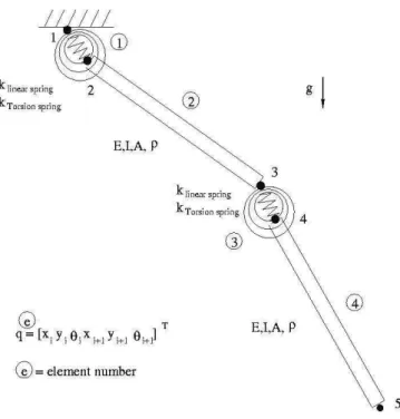
Before to face the proposed biomechanical problem, some tests are made on a simpler model where the formulation is easier and results are more conclusive. This proposed model example is shown in Fig. 1. Despite its geometric simplicity, it can bring all sort of difficulties expected in a biomechanical model. It's composed of two flexible bars linked by a torsional and linear spring element. One of the bars is attached to a fixed point through a spring element, similar to the previous but having different stiffness. The spring element stiffness will be the parameters p to identify.
Figure 1. Two flexible bars linked by spring elements.
The following data were given to this problem: bar's Young modulus E=2.1x10¹⁰ Pa, section area A=25x10-6 m2, inertia section I=52.1x10⁻¹² m4, bar's volume density ρ=7800 kg/m3, bar's initial length Lb=0.9 m, non extended spring length Ls=0.1 m, ktorsional=0.5 Nm/rad, klinear(elt 1)=700 N/m, klinear(elt 3)=400 N/m. The exact set of parameters to identify is then
J. of the Braz. Soc. of Mech. Sci. & Eng. Copyright 2006 by ABCM October-December 2006, Vol. XXVIII, No. 4 /471 The only solicitations are the gravity forces. The initial situation
consists in letting this whole multibody system falling freely from a same initial angle of bars and springs with respect to a vertical line equal to π/6. The DAE are integrated for 3s using the HHT scheme presented before. All nodal kinematics responses q ,q ,qɺɺ ɺt t t are registered as our simulated set. We generate our measured set by using only the set qt. Derivative qɺt and ɺɺqt are obtained by finite
central difference method from qt.
We decided to apply the three temporal identification methods starting from a vicinity of our parameter solution.
We test the direct and the indirect identification procedures at times t1=0,69 s and t2=2,83 s. These times were close and far, respectively, from the starting state. They were also defined according to a criterion of bad numerical evaluation meaning that at times chosen difference between simulated and measured responses is the greatest.
For the adapted procedure, because it is analyzed separately, the first time instant set is taken in the first third of time simulation [0.5s 1.0s]. Then, two sets of five instants [0.6s 0.9s 1.4s 2.1s 2.7s]
and [0.4s 1.1s 1.6s 1.9s 2.3s] are taken in a more or less distributed form between 0s and 3s.
Results and Conclusions
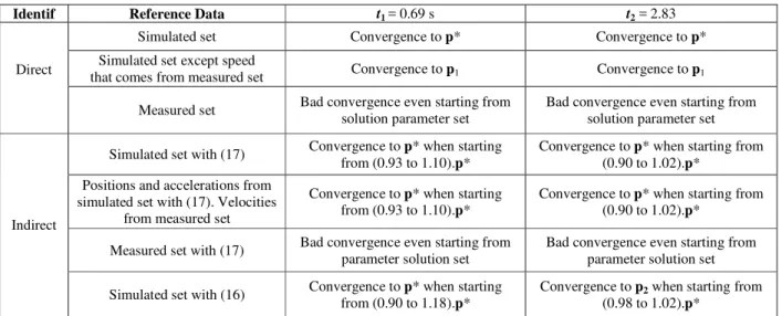
The indirect identification procedure was performed with the two residues presented in Eq. (16) and Eq. (17). In Eq. (16) only the nodal position variables were used in q t
( )
and q( )
t , as an example we test the procedure with qT=x2 y4 x5 y5T and[
]
TT x y x y
5 5 4 2
=
q . This has been done in order to evaluate the capabilities of the procedure when dealing with a reduced residue vector.
The simulated and the measured sets are used consecutively as measured data to perform the identification. Several starting sets of parameters between 0.8 p* and 1.2 p* are chosen for the optimization procedure. Identification evaluations were summarized in Tab. 1.
Table 1. Tests results.
Identif Reference Data t1 = 0.69 s t2 = 2.83
Simulated set Convergence to p* Convergence to p* Simulated set except speed
that comes from measured set Convergence to p1 Convergence to p1 Direct
Measured set Bad convergence even starting from solution parameter set
Bad convergence even starting from solution parameter set
Simulated set with (17) Convergence to p* when starting from (0.93 to 1.10).p*
Convergence to p* when starting from (0.90 to 1.02).p*
Positions and accelerations from simulated set with (17). Velocities
from measured set
Convergence to p* when starting from (0.93 to 1.10).p*
Convergence to p* when starting from (0.90 to 1.02).p*
Measured set with (17) Bad convergence even starting from parameter solution set
Bad convergence even starting from parameter solution set Indirect
Simulated set with (16) Convergence to p* when starting from (0.90 to 1.18).p*
Convergence to p2 when starting from (0.98 to 1.02).p*
With the solution sets being p1=[663 0.49 379 0.49]T and
p2=[757 0.50 465 0.52]T. In table 1, a "Bad convergence" means that the identified set of parameters has no mechanical signification; a negative Young modulus as example.
The results show that the direct identification procedure is very sensible to modified acceleration values but less to velocities. Nevertheless, a small modification of velocities, due to the finite difference scheme for derivation, causes an error on the identified parameter set: p1 instead of p*.
The indirect procedure proposes a very interesting alternative with allowing to not use accelerations. Nevertheless, the starting set of parameters for the optimization procedure has to be very close from the expected response.
The simulation time also plays an important role in the results obtained. We could verify that the more the simulation time is big the more the starting point has to be near of the solution to convergence. This can be explained by the great differences, especially in trajectory accelerations, generated by different parameter sets. Moreover, the time processing is strongly linked to time simulation for the indirect procedure.
Figure 2. Displacements sensibilities.
Figure 3. Velocities sensibilities.
Figure 4. Accelerations sensibilities.
Figure 5 shows the sensibility of forces in x and y directions and of the torque to parameters in the first element spring. It is interesting to notice here that even if force responses are dependent from the parameter sets, the levels of force magnitudes are not.
Figure 5. Forces sensibilities.
For the adapted direct identification procedure, evaluations are summarized in Tab. 2. The linear stiffness always converges towards the solution values, even for the reduced instant set. Further, their convergence are also verified for departure points far from the solution values (30 p*). This means that those parameters strongly affect the studied dynamic system behavior. In the other hand, the variation in torsional stiffness does not seem to play an important role in the system equations, especially when short instants sets are used, i.e. few equations are employed in the optimization procedure.
Table 2. Parameter solution for different instant sets.
Instant set Identified p
[0.5s 1.0s] [700 –0.47 400 5.10] [0.6s 0.9s 1.4s 2.1s 2.7s] [700 0.42 400 0.58] [0.4s 1.1s 1.6s 1.9s 2.3s] [700 0.51 400 0.58]
The nodal relative rotations ∂θi=
(
θi−θi)
/θi and the relative Lagrange parameter ∂λθ =(
λθ−λθ)
/λθ obtained after the optimization procedure, are shown in Tab. 3 for the third instant set [0.4s 1.1s 1.6s 1.9s 2.3s]. The Lagrange parameterλ
θ concerns the torsion reaction at node 1 (Fig. 1).Table 3. Relative errors (x103) of rotations and Lagrange parameter.
ti cθ2 cθ3 cθ4 cθ5 cλθ 0.4s 0.05 0.1 0.1 0.04 1.68 1.1s 0.06 0.07 0.05 0.02 5.68 1.6s 0.01 0.06 0.04 0.02 1.88 1.9s 0.01 0.03 0.03 0.02 3.42 2.3s 0.1 0.19 0.17 0.07 4.05
One can see that some parameters, and especially the coefficients of the employed interpolation functions, are well determined meaning they also have considerable weight in dynamic equations what is not true for the rotation time derivatives. The results have revealed this can be a good and simple manner of identifying kinematics, dynamic, physic and geometric parameters in multibody flexible dynamic systems when the rotation data are not provided.
J. of the Braz. Soc. of Mech. Sci. & Eng. Copyright 2006 by ABCM October-December 2006, Vol. XXVIII, No. 4 /473 good alternative to follow due to its similarity with the available
data of the original biomechanical problem. However, more powerful search methods are required to overcome the uncertainties of the departure searching point when the answer is not known. Future tests, using many reference times and introduced noise in position reference data, will be performed to verify how those changes can affect the response quality and the departure point range of parameter set. At last, the adapted direct procedure presents good identification capabilities but have to be investigated for more instant sets. Its robustness has to be verified with measurement noises.
We still have to take into account the fact that temporal integration schemes impose modification of the equilibrium equation to solve. It is well known that these schemes present numerical dissipation due to the damping coefficient introduced to filter high frequencies causing the instabilities. But even conservative schemes present defects as phase error. To give a mechanical meaning of the parameters evaluated, this drawback has to be included in the identification procedure when simulated data are compared to measured ones. Nevertheless, we are great confident in the recent development in the simulation of MBS (Schiehlen, 2005)(Ibrahimbegovic & al., 2003) and we will focus our future investigations on the identification process.
Acknowledgements
Thanks to Haut Normandy Region (France) for funding this work through Research Department of CHU de Rouen.
References
Mejjad, O., Dujardin, F., Leloet, X., Weber, J., Thomine, J.M., 1998, "Hip joint kinematics during gait in hip osteoarthritis, versus healthy subjects", American College of Rheumatology (ACR) – San Diego CA, USA Dujardin, F., Toupin, J.M., Duparc, F., Biga, N., Thome, J.M., 1997, "Correlation entre la cinématique coxo-femural au cours de la marche et l'usure du couple de frottement des prothèses type Charneley-Kerboull",. Rev. Chirurgical orthop., Suppll. II 83-43.
Dhatt, G. and Batoz, J.L., 1990, “Modélisation des structures par éléments finis : poutres et plaques” , Hermes, Vol. 2.
Crisfield, M.A., 1991, “Non-Linear Finite Element Analysis of Solids and Structures: Essentials”, John Wiley & sons, Vol. 1.
Jalon, J.G. and Bayo, E., 1994, "Kinematic and Dynamic Simulation of Multibody Systems", Springer–Verlag Mechanical Engineering Series
Geradin, M. and Cardona, A., 2000, “Flexible Multi-body Dynamics: A Finite Element Approach”, John Wiley & sons.
Schiehlen, W., 2005, "Recent developments in multibody dynamics", Journal of Mechanical Science and Technology, Vol.19, n°1, pp. 227-236.