Abstract
In this study a total lagrangian 2D finite element formulation is used to model plane frames developing large displacements and rotations considering sliding connections. This kind of connections is usually called prismatic and cylindrical joints.
In order to be self-containing, the steps of the development of a frame finite element of any approximation order that considers the influence of shear strain by means of a generalized Reissner kine-matics is presented. The adopted degrees of freedom are positions and rotations. Using positions as degrees of freedom simplifies the total lagrangian description and enables a comprehensive presen-tation of the proposed connections. Revolute connections are con-sidered by direct degrees of freedom matching. Prismatic connec-tions are modelled by the Lagrange multiplier technique that constrains positions and rotation of a sliding node to the varying position and rotation of a path element. Cylindrical joints are introduced in similar way by Lagrange multipliers releasing the sliding node rotation.
The principle of stationary potential energy is used to write the non-linear equilibrium equation including the Lagrange multiplier influence. To solve the non-linear equation a Taylor expansion is carried out and the Newton-Raphson procedure is employed. The frame element is considered elastic, following the Saint-Venant-Kirchhoff constitutive model. Selected examples are used to vali-date the formulation and to show its possibilities of application.
Keywords
Positional Finite Element Method, Sliding connections, Lagrange multipliers.
Development of Sliding Connections for Structural
Analysis by a Total Lagrangian FEM Formulation
1 INTRODUCTION
Considering the constant evolution of materials science, the use of materials with improved mechan-ical properties is a reality in daily engineering applications. Therefore, the design of audacious
struc-Tiago Morkis Siqueira a, * Humberto Breves Coda a, **
a Structural Engineering Department,
Escola de Engenharia de São Carlos, Universidade de São Paulo
Corresponding author:
* [email protected] ** [email protected]
http://dx.doi.org/10.1590/1679-78252494
tures each time slenderer and lighter is a constant challenge for engineering. From this point of view, the consideration of geometrical non-linearity in structural analysis is becoming an imposition nowadays. On the other hand, the analysis of deployable and bi-stable structures is also an im-portant field of mechanical and aerospace engineering. Some applications as satellite antennas, de-flectors, solar panels and solar sails are designed using the concept of sliding connections, large dis-placements and rotations.
As far as the authors knowledge goes, differently from what is proposed in this study, all exist-ing finite element method (FEM) formulations related to this kind of connection that considers large displacements and rotations are based on the updated lagrangian concept, more specifically co-rotational formulations. Those formulations are presented in the works of Simo and Vu-Quoc (1986), Armero (2006), Jelenic and Crisfield (2001) and Ibrahimbegović and Taylor (2002). Moreo-ver, the specific developments of mathematical models of such connections are in its majority relat-ed to multibody dynamics, becoming a hard path to researchers not trainrelat-ed on this subject (Bauchau, 1998; Cardona; Géradin; Doan, 1991; Géradin; Cardona, 2001; Sugiyama; Escalona; Shabana, 2003). This approach may create a dependence of dynamic analysis when some simple static modelling could be of interest to describe low velocity mechanical systems or sliding connec-tions in statics. We could find one static work, Jelenic and Crisfield (1996), that takes care of static 3D connections, however the connections are written regarding nodal variables and limits the movement to straight directions not associated to the flexibility of structural members.
One can see, for example, in Bauchau (2000) and Bauchau and Bottasso (2001) the use of La-grange multipliers to solve sliding joints in dynamic analysis, however, the application of constraints are done directly at the equilibrium level and the non-linear solution process is not detailed. Moreo-ver, the authors decided to use non-dimensional variables as the main unknowns of the problem, limiting the sliding equations to one single element and introducing some difficulties on the interpre-tation of forces and mass values at the joint node. In the works of Bauchau (1998), Cardona, Géra-din and Doan (1991), Bauchau (2000) and Bauchau and Bottasso (2001) the Hamilton principle is used to derive the elastodynamic equations for the geometrical non-linear FEM formulation dedicat-ed to elastic multibody dynamics. Some comments about difficulties regarding using the Newmark method for time integration and the proposition of energy conserving algorithms are also described in literature on Bauchau (1998), Cardona, Géradin and Doan (1991), Romero and Armero (2002) and Leyendecker, Betsch and Steinmann (2006). Other interesting works related to multibody dy-namic applications can be mentioned such as Greco and Coda (2006), Yoo et al. (2007), Hong and Ren (2011) and Moon et al. (2014).
cylindri-cal joint model. Moreover, the main variable at the connection of elements respects the Euclidean space dimension and consistent results are achieved.
The non-linear equilibrium equation is derived from the stationary total potential energy prin-ciple and solutions along the equilibrium path are achieved by means of the Newton-Raphson pro-cedure. Selected examples are presented to validate the formulation and to show its possibilities of application.
2 PLANE FRAME KINEMATICS
The adopted FEM solution procedure is written here from the principle of stationary potential en-ergy and, therefore, the strain enen-ergy stored in the frame element must be calculated. To calculate the strain energy, it is necessary to define the way one achieves the strain distribution as a function of the body position limited to a finite number of degrees of freedom. In order to do so we write the initial and current positions of frame elements as a function of nodal position, angles and non-dimensional variables.
2.1 Initial Configuration
To build the total lagrangian procedure we start describing the initial configuration of a frame ele-ment. Figure 1 shows the reference line of the initial configuration, the non-dimensional space from which the reference line mapping is written and the nodes of the finite element.
The mapping of the reference line is written as:
0mi( ) im( ) ( ) im
f x =x x =f x X , (1)
where, i is the direction (1 or 2), m indicates reference line and is the index that represents nodes and shape functions f x( ) (Lagrange polynomials of any order). Xim represents the nodal
coordinates at the reference line and repeated indices indicate summation.
Figure 1: Reference line parameterization for initial position (cubic approximation).
0m( ), ( ) f f f
11 21 ( , )m m
x x 1
1 x 2
x
0 1
1 T 1
N
12 22 ( ,m m)
x x 2
0 2
2 T 2
N
13 23 ( , )m m
x x 3
0 3
3
T 3
N
14 24 ( , )m m
x x 4 40
4 T 4
N
1
At the initial configuration, the nodal coordinates are known and the cross sections are consid-ered orthogonal to the reference line. Thus, from figure 1, one calculates the tangent vectors at each node k by:
, ( ) , ( )
m m m
ik i k k i
T =x x x =f xx X, (2)
in which comma indicates derivative.
From equation (2) the normal vectors that generate cross sections at nodes are written as:
1k 2k / and 2k 1k /
N = -T T N =T T , (3)
where the index m has been omitted. To use angles as nodal parameters, one calculates, from
fig-ure 1:
0
2( ) 1( )
( / )
k arctg N k N k
q = (4)
To define a cross section at any position along the frame element it is necessary to know its an-gles. In order to do so we use the same approximation adopted for coordinates, i.e.:
0( ) ( ) 0
q x =f x q (5)
From the initial position of reference line and cross sections orientation one defines the initial configuration of the frame element as depicted in figure 2.
Figure 2: Initial configuration mapping.
One can deduce from figure 2 that the initial configuration mapping is written using a non-dimensional space
(
x h,)
by:( , ) f f f
1
x
2
x
0 2
h
0 2
h
0 2
h
0 2
h
reference line
0
x1m ,x2m
x1 , ,x2 ,
cross
section
1
0 1 1
1 0
0( , )
0 ( , ) m( ) ( , )
i i i
x x h =x x +g x h , (6)
where the vector 0( , )
i
g x h can be written as a function of q x0( ), h and the height 0
h of the finite element as:
0 0 0 0 0 0
1( , ) cos ( ) and 2( , ) sen ( )
2 2
h h
g x h = h éëêf x q úùû g x h = h êéëf x q úùû (7)
Substituting equations (1) and (7) into equation (6) results the initial configuration mapping of the frame element, as:
0 0
01( , ) 1( , ) ( ) 1 cos ( )
2
m h
f x h =x x h = f x X + h éêëf x q ùúû (8)
0 0
02( , ) 2( , ) ( ) 2 sen ( )
2
m h
f x h = x x h =f x X + h éêëf x q ùúû (9)
It is worth noting that, for the sake of simplicity, the reference line is adopted at the centre of the cross section and the width and height of the bar are considered constant along all frame ele-ment. One can adopt the reference line at any position and the internal force offsets would appear naturally (Coda; Sampaio; Paccola, 2015; Pascon; Coda, 2013).
2.2 Current Configuration
The current configuration is understood as a trial position of the solution process and can be seen in figure 3.
Figure 3: Current configuration mapping.
y
2
y
reference line
1( , )
f f f
1
0 1 1
1 0
0 2
h
0 2
h 1
1
2
2
3
3
4
4
Therefore, the new nodal coordinates m i
Y and angles q can be used to derive the current mapping from the non-dimensional space
(
x h,)
to the current configuration as:0
11( , ) 1( , ) 1 cos[ ( ) ]
2
m h
f x h = y x h = fY + h f x q (10)
0
12( , ) 2( , ) 2 [ ( ) ]
2
m h
f x h =y x h = fY + hsenf x q (11)
where f1i( , )x h =yi( , )x h is the new mapping understood as the current positions of any point inside the body at the current configuration mapped from the non-dimensional space.
As, at current configuration, there is no relation between q and the reference line inclination, see figure 3, the cross section is not orthogonal to the reference line, consequently, Reissner kine-matics takes place. It is worth noting that the height of the frame element is not free to change and, to avoid volumetric locking the constitutive equation should be relaxed in order to exclude trans-verse expansions.
2.3 Complete Mapping and Green Strain
After defining the mappings from the non-dimensional space to the initial B0 and current B
con-figurations, we introduce the mapping from the initial configuration to the current configuration in the same sense presented by Bonet et al. (2000) and Coda (2003). In figure 4 we put together fig-ures 2 and 3 revealing the mapping f as:
1 1 ( )0
f = f f - , (12)
where f0
(
x h,)
and f1(
x h,)
are defined by equations (8) to (11).Figure 4: Change of configuration function or deformation function. 0
( )
f f f
0
f f f
1, 1
x y
2, 2
x y
0
B
B f f f
1
To calculate strain and strain energy it is not necessary to explicitly know f, but its gradient, called here A. This is done in a very simple way (Bonet et al., 2000; Coda, 2003) as:
1. ( 0)-1
=
A A A , (13)
in which
0 0 1 1
1 1 1 1
0 1
0 0 1 1
2 2 2 2
and
f f f f
f f f f
x h x h
x h x h
é¶ ¶ ù é¶ ¶ ù
ê ú ê ú
ê ¶ ¶ ú ê¶ ¶ ú
ê ú ê ú
=ê ú =ê ú
¶ ¶ ¶ 
ê ú ê ú
ê ¶ ¶ ú ê¶ ¶ ú
ë û ë û
A A (14)
For a trial current nodal position, both A0 and A1 are numerical values at a generic point
(
x h,)
. In the numerical strategy, coordinates(
x h,)
are Gauss integration points resulting in a very simple numerical procedure. Moreover, expression (14) indicates that there is no difference model-ling straight or curved elements by the proposed formulation.Substituting equations (8), (9), (10) and (11) into equation (14) results:
0 0 0 0 0
, 1 k,
0
0 0 0 0 0
, 2 k,
( ) ( ) ( ) cos ( )
2 2
( ) cos ( ) ( ) ( )
2 2 m k m k h h X sen h h X sen x x x x
f x h f x q f x q f x q f x h f x q f x q f x q
é é ù é ùù
ê - ê ú ê úú
ê ë û ë ûú
= ê ú
ê + é ù é ùú
ê êë úû êë úûú
ê ú
ë û
A
(15)
0 0 0 0 0
, 1 k,
0
0 0 0 0 0
, 2 k,
( ) ( ) ( ) cos ( )
2 2
( ) cos ( ) ( ) ( )
2 2 m k m k h h X sen h h X sen x x x x
f x h f x q f x q f x q
f x h f x q f x q f x q
é é ù é ùù
ê - ê ú ê úú
ê ë û ë ûú
= ê ú
ê + é ù é ùú
ê êë úû êë úûú
ê ú
ë û
A
(16)
The Green-Lagrange strain E is adopted to develop the formulation, as it is an objective
meas-ure (Ogden, 1984), and is given by:
1 1 1
( ) ( ) or ( )
2 2 2
t
ij ki kj ij
E A A d
= - = ⋅ - =
-E C I A A I (17)
In which I is the identity tensor of second order and C is the right Cauchy-Green stretch.
3 EQUILIBRIUM EQUATION
As mentioned in the introduction, the equilibrium equation is achieved here from the principle of stationary energy. For the considered isothermal, static and elastic situation the total energy is written as:
e
U P
P = + , (18)
where
P
is the total energy of the system, Ue is the stored elastic energy and P is the potential of0 e
U P
dP =d +d = , (19)
in which the symbol d means variation.
3.1 Strain Energy Adopted to the Proposed Frame Element
In order to calculate the strain energy of the analysed body (frame element) it is necessary to inte-grate over the initial volume (lagrangian formulation) the specific strain energy written here as a function of the Green-Lagrange strain (E) as:
(
)
(
)
2 2 2 2 C
11 22 12 21
1
or : :
2 2
e e
u = E +E + E +E u = E E, (20)
where is the longitudinal elastic parameter of the Saint-Venant-Kirchhoff constitutive model that approaches the Young modulus for small strain. The shear elastic modulus is = [2(1+n)] being n a constant that reproduces the Poisson ratio for small strain. As one can see, in the present formulation the Poisson ratio interferes only on the shear stiffness and does not introduces trans-verse expansion. The energy conjugacy property allows one to define the second Piola-Kirchhoff stress as:
S e or e
ij
ij
u u
S
E
¶ 
= =
¶E ¶ , (21)
moreover, the constitutive elastic tensor C can be achieved as:
E E
C = C
2 2
or
e e
ijk
ij k
u u
E E
¶ 
=
¶ ¶ ¶ ¶ (22)
It is worth noting that the adopted constitutive model avoids volumetric locking and that the high order of finite elements avoids shear locking (Bischoff; Ramm, 2000).
As the Green strain has been written as a function of nodal positions, see equations (15), (16) and (17) the strain energy accumulated in the structure is also a function of positions, and is writ-ten as:
0 0
( ) ( )
e V e
U Y =
ò
u Y dV , (23)in which V0 is the initial volume of the frame.
3.2 Total Potential Energy and Equilibrium
The total potential energy of the mechanical system in an elastic, static and isothermal condition ( )Y
P is given by the sum of the strain energy and the potential energy of external forces, as:
0 0
0 0
( ) ( ) m
e
V S
Y u Y dV F Y q y dS
In this expression F is the conservative applied forces (including moments), q is the vector of ex-ternal distributed forces written as a function of nodal values as
q
i=
f x
( )
Q
i, ym is the current position of the reference line (Equations (10) and (11)) and dS0 is the initial infinitesimal reference line length of a curved frame element.To achieve the equilibrium equation one applies the principle of stationary potential energy on expression (24) using nodal positions as parameters,
0 0 0 0
( ) ( )
( ) 0
m e
V S
u F Y q y
Y YdV Y YdS
Y Y Y
dP = ¶ ⋅d -¶ ⋅ ⋅d - ¶ ⋅ ⋅d =
¶ ¶ 
ò
ò
(25)
Knowing that the strain energy is a function of Green strain which is a function of positions, and that the applied forces are conservative, equation (25) is rewritten as:
0 0 0 0
( ) : 0
m e
V S
u y
Y YdV F Y q YdS
Y Y
dP = ¶ ¶ ⋅d - ⋅d - ⋅¶ ⋅d =
¶ ¶ 
ò
E Eò
(26)
Knowing the current reference line expression (ym = ⋅f Y), the adopted surface force
approx-imation (q = f ⋅Q) and equation (21), one writes equation (26) as:
0 0 0 0
( ) : 0
V S
Y YdV F Y Q YdS
Y
dP = ¶ ⋅d - ⋅d - ⋅f Ä ⋅f d = 
ò
S Eò
, (27)
in which the symbol Ä represents the tensor product.
It is usual to write equation (27) as (Coda; Paccola, 2014): int
( )Y F Y F Y Q Y 0
dP = ⋅d- ⋅d- ⋅L ⋅d = , (28)
in which
F
int represents nodal forces and L is the matrix that transforms distributed forces intonodal equivalent ones (Coda; Paccola, 2014). As the variation dY is arbitrary, equation (28) results
in the geometrical non-linear equilibrium equations for discrete frame analysis, as:
int 0
F -F- ⋅L Q = (29)
3.3 Piola-Kirchhoff Stress and Green Strain Derivatives
In order to be possible the reproduction of the proposed formulation it is important to show how the kernels of equation (27) are calculated. The second Piola-Kirchhoff stress S is obtained from
equations (20) and (21) as:
1112 2212 2 2
e E E
u
E E
é ù
¶ ê ú
= = ê ú
¶ êë úû
S
E (30)
0 1 1 0 1
1 1
0 1 0 1 0 1 0 1
1 1 1
( ) [( ) ( ) ( ) ]
2 2 2
( )
1
( ) ( ) ( ) ( ) ( )
2
t t t
t
t t t
Y Y Y Y
Y Y - -- - - -¶ ¶ ¶ ¶ = = ⋅ = ⋅ ⋅ ⋅ ¶ ¶ ¶ 
é ¶ ¶ ù
ê ú
= ê ⋅ ⋅ ⋅ + ⋅ ⋅ ⋅ ú
¶ 
ê ú
ë û
E C
A A A A A A
A A
A A A A A A
(31)
As ¶(A1) /t ¶Y = ¶( A1 /¶Y)t one can simplify equation (31). From equation (15) it is possible to derive A1 regarding nodal positions Yb
a , for which a is the direction (1, 2 or 3, for the angle) and b is the element node, as follows:
1 1
1 2
0 0 0
,
0 0 0
Y Y
b
b b b
f
f
é ¢ ù é ù
¶ ê ú ¶ ê ú
= ê ú =ê ¢ ú
¶ êë úû ¶ êë úû
A A
(32)
0 0 0
1 1
0 0 0
3
cos( ) ( ) ( ) ( )
2 2 2
cos( ) ( ) ( ) cos( )
2 2 2
k k
k k
h h h
sen sen
h h h
Y sen
b b b
b b
b b b
h f q f f q h f q f f q f q h f q f f q h f q f f q f
é ù
ê- ¢ - ¢ - ú
¶ = ¶ ê ú
= ê ú
¶ ê ú
¶ ê- ¢ + ¢ ú
ê ú
ë û
A A
, (33)
with summation over nodes
and k .From expressions (30) through (33) the internal force is calculated using Gaussian quadrature over the initial volume, as:
(
)
int 0
0 ig jg ( ig, jg) : (ig, jg) (ig, jg)
F b w w Det
Y
x h ¶ x h x h
=
¶ E
S A
, (34)
in which wig and wjg are Gauss weights and xig and hjg are integration points.
4 SOLUTION OF THE NON-LINEAR EQUILIBRIUM EQUATIONS
In order to organize the solution procedure, based on the Newton-Raphson method, one rewrites equation (29) coupling external forces in one unique vector F, as:
int 0
g =F -F = (35)
In this expression g is called the unbalanced mechanical force vector, as it is null only when the position Y is the solution of the problem.
Equation (35) can be understood simply by finding Y such that g Y( ) = 0. This statement is clearly non-linear regarding Y. Therefore, to find a solution of the problem one expand the equality
in a Taylor series truncated at the first order,
0 0
( ) ( ) ( ) 0
g Y @ g Y + g Y ⋅ DY = , (36)
in which Y0 is a trial solution.
Solving the linear system of equation (36) one finds a correction DY to the trial solution as:
1 ( 0)
Y - g Y
where the gradient of g is the Hessian of the total potential energy. As the external forces are con-servative, the Hessian matrix is given by:
2 2
e U g
Y Y Y Y
¶ ¶ P
= = =
¶ ¶ H ¶ 
(38)
Using DY, a new trial position is achieved, as:
0 0
Y =Y + DY (39)
This new trial solution is used again in equation (37) until:
( )
or
g Y Y
TOL TOL F X D £ £
, (40)
when Y =Y0 is assumed to be the acceptable solution of (35). In equation (40) X is the Euclidi-an norm of the initial position vector.
4.1 Hessian of the Proposed Frame Element
To complete the description, the frame element Hessian matrix H is presented as:
0 0 0
2 2 int 2
0 0 : : 0
e e
V V V
U u F
dV dV dV
Y Y Y Y Y Y Y Y Y
æ ö
¶ = ¶ = ¶ = çç¶ ¶ + ¶ ÷÷÷
ç ÷÷
ç
¶ 
ò
¶ ¶ò
¶ò
è¶ ¶ ¶ ¶ øS E E
S
(41)
In the last integral, the derivative of the Piola-Kirchhoff stress ¶ ¶S Y is given by:
11 12
11 12
21 22 21 22
2 2 2 2 E E E E Y Y
E E E E
Y Y
Y Y
é ¶ ¶ ù
ê ú
é ù ê ú
¶ ¶ ê ú ¶ 
= ê ú= ê ú
¶ 
ê ú
¶ ¶ êë úû ê ú
ê ú
ë ¶ ¶ û
S
, (42)
for which the derivatives of the Green strain regarding positions is already given in equations (31) and (32).
Thus, the last term to be achieved is the second derivative of the Green strain regarding posi-tions, i.e.:
1
2 1
0 ( ) 0 1
1
2( ) ( )
2
t
t t
Y Y Y Y
-
-é ¶ ù
¶ = ê ⋅ ⋅¶ ⋅ + + ú
ê ú
¶ ¶ êë ¶ ¶ úû
A
E A
A A O O
, (43)
with,
2 1
0 1 0 1
( ) t ( )t ( ) Y Y
- 
-= ⋅ ⋅ ⋅
¶ 
A
The non-null values of ¶2A1 /¶ ¶Y Y are restricted to the third direction (angles) and are given by:
{
}
{
}
2 1 2 1
3 3
0 0
0 0
( ) ( ) cos( ) cos( )
2 2
cos( ) ( ) ( ) ( )
2 2
k k
k k
Y Y
h h
sen
h h
sen sen
z b
b z
b z b z b z b z
b z b z b z b z
q q
h f q f f f q f q f f f f f q f f h f q f f f q f q f f f f f q f f
¶ = ¶ =
¶ 
¶ 
é ù
é ù
ê ¢ - êë ¢ + ¢ úû - ú
ê ú
= ê ú
ê- ¢ + é ¢ + ¢ ù - ú
ê êë úû ú
ê ú
ë û
A A
, (45)
where b and z are element nodes and summation over and k are present. The integration over elements is given by Gaussian quadrature, as:
2 2
0
0 ( , ) : ( , ) ( , ) : ( , ) ( , )
e
ig jg ig jg ig jg ig jg ig jg ig jg
U
b w w Det
Y Y Y x h Y x h x h Y Y x h x h
é ù
¶ ê¶ ¶ ¶ ú
= ê + ú
¶ ¶ êë¶ ¶ ¶ ¶ úû
S E E
S A
, (46)
for which wig and wjg are weights and xig and hjg are integration points.
5 SLIDING CONNECTIONS
As mentioned in the introduction section, revolute connections are not sliding ones and are consid-ered by the direct matching of degrees of freedom, readers are invited to see the references Greco and Coda (2006), Reis and Coda (2014) and Coda and Paccola (2014) for details.
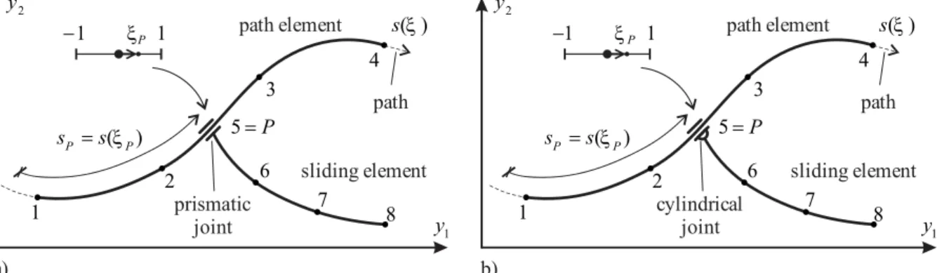
A prismatic joint, schematically depicted in figure 5a, constrains the extremity position of the sliding element to slide over a path element without allowing relative rotation. A cylindrical joint constrains the extremity of the sliding element to slide over a path element but releases the relative rotation between elements, see figure 5b.
We describe in details the prismatic connection, for which Lagrange multipliers are used to con-strain positions and relative angles. The cylindrical connection is briefly described indicating which terms of the prismatic joint are disregarded. One important advantage of using Lagrange multipli-ers is the simplicity of the technique when considering the principle of stationary total potential energy and the total lagrangian description.
5.1 Kinematical Constraints by Lagrange Multiplier
A set of path elements defines the sliding path of the connected node of a sliding element, this con-nected node is now on called sliding node. In what follows ( )· is used for path elements and ( )ˆ· for sliding elements, including the sliding node.
Figure 5: (a) Prismatic joint, (b) cylindrical joint.
The variable sp =s
( )
xp , depicted in figure 5, defines the curvilinear position and the crosssec-tion orientasec-tion of the path point P (with coordinates P i
Y ) over the sliding path. For cylindrical connections the cartesian coordinates (ˆP
î
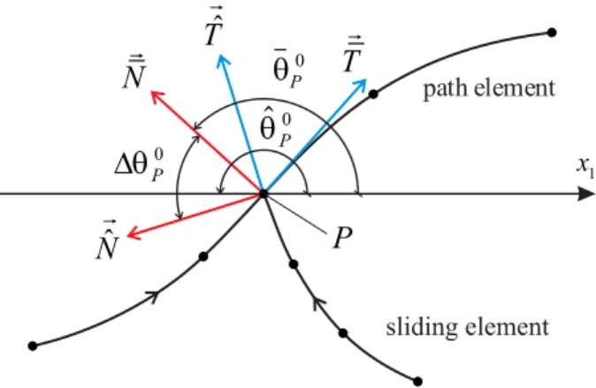
Y ) of the sliding node Pˆ should be equal to the cartesian coordinates of point P belonging to the sliding path. For prismatic connections, in addition to posi-tions, the difference of cross sections orientations 0
p
q
D , calculated at the initial configuration (figure 6), should be constant during the sliding process. These constraints are described by:
( )
(
)
(
( )
)
( )
( )
ˆP m m m for 1, 2
i i p i p i p P i
Y =y s x =y x s =y x = f x Y i= , (47)
and,
0 ˆ ( ) ˆP ( ) 0 for 3
P P P or Yi P Yi P i
q q f x q f x q
D = - = + D =
, (48)
or, in a general, form:
( )
(
)
( )
03
ˆP ,
i P i P i P i
Y s x Y = f x Y + Dq d , (49)
where di3 is the Kronecker delta.
During sliding, the curvilinear position sp =s
( )
xp or, inversely, the non-dimensional coordinate( )
p sp
x =x will vary.
To impose the kinematical constraint of a prismatic joint via Lagrange multiplier one adds to the total potential energy the following potential:
joint
sliding element path path element
1
P 1
( )
P P
s s
( ) s
1
2
3
4
5P 6
8 7
1
y
2
y
cylindrical joint
sliding element path path element
1
P 1
( )
P P
s s
( ) s
1
2
3
4
5P 6
8 7
1
y
2
y
( )
(
)
0
3 ˆ
( , , ) P
L p i i p i P i
Y s l =l ëêéY -f x s Y - Dq d ùúû, (50)
in which the term inside brackets is exactly the kinematical constraint given by equation (49), li
are the so called Lagrange multipliers, one for each direction i (summation implied), and YL repre-sents the connected positions. In mechanics an interesting physical interpretation can be given for the Lagrange multiplier, that is, its converged value is the auto equilibrated force (action and reac-tion) necessary to keep both bars together.
Figure 6: Difference of angles for a single node at different elements.
The new potential energy is written as:
0 0 0 0
( , ) ( ) m ( , )
LY L V u Y dVe F Y S q y dS Y LL
P =
ò
- ⋅ -ò
⋅ + , (51)in which Y include all degrees of freedom, less the new ones L =
(
sp,l)
as YL is already included in Y. The principle of stationary potential energy is applied on expression (51) to find equilibriumequations, as:
0
L
dP = P +d d = , (52)
in which dP has already been detailed in previous sections and include variations of the strain en-ergy and applied external forces regarding current nodal positions Y.
To complete the variation of PL( , )Y L it is necessary to solve d. This is done regarding
(
p,)
L = s l and
(
, ˆP)
L i i
Y = YaY :
( )
( ) ˆ ˆ ( )
P
L i P i i P
i P
L i i
Y L Y Y s
s
Y L Y Y
a a
d d d d d dl d
l
¶ ¶ ¶ ¶ ¶ 
= + = + + +
¶ 
¶ ¶ ¶ 
, (53)
being a the nodes of the active path element. One should note that variable YL
belongs to Y and
will result in terms to be added in internal force and Hessian matrix at the solution process. At this,
path element
1
x
ˆ
T
T
ˆ
N
N
0 P
P
0 P
0 P
it is important to mention that the consulted works that deal with flexible connections use xp in-stead of sp as the main variable.
For prismatic connections, developing the derivatives, one writes in an open form:
{
}
( )
( )
( )
0 3 ,ˆ ˆ 0 1, 2, 3
ˆ / i P i P k k
i i i i p
P
i P i P i
i P i P
L Y Y Y s i
Y Y
Y J
a
a
x
l f x l d d d d d dl d
f x q d
l f x
ì - ü
ï ï ï ï ï ï ï ï ï ï ï ï ï ï ï ï
= L ⋅ = íï ýï =
ï - - D ï
ï ï
ï ï
ï ï
ï - ï
ï ï ï ï î þ , (54)
in which the nodes belonging to the sliding element, different from the sliding node, represented by index k are present in equation (54) in order to simplify the 'Lagrange Force' vector L assem-blage.
In equation (54) the following property is used,
( )
or p( )
p p p
ds
ds J d J
d
x x x
x
= = , (55)
in which,
( )
( )
2( )
2, 1 , 2
[ ] [ ]
p P P P
J x =J = fx x Y + fx x Y (56)
The new equilibrium equation is now assembled respecting the degrees of freedom correspond-ence adding L to Fint, i.e.:
(
Fint + L -)
F = 0,(57)
in which F includes all external loads.
For cylindrical connections, the same procedure is used, remembering that the relative angle is free, resulting:
{
}
( )
( )
( )
,ˆ ˆ 0 1, 2
ˆ / i P i P k k
i i i i p
P
i P i
i P i P
L Y Y Y s i
Y Y
Y J
a
a
x
l f x l d d d d d dl d
f x l f x
ì - ü
ï ï ï ï ï ï ï ï ï ï ï ï ï ï ï ï
= L ⋅ = íï ýï =
ï - ï
ï ï
ï ï
ï ï
ï- ï
ï ï ï ï î þ (58)
5.2 Non-Linear Solution
The non-linear set of equilibrium equations (57) is also solved by the Newton-Raphson procedure. The unbalance mechanical vector gL
is written as:
(
,)
(
int)
0L
For a trial solution
(
0, 0)
Y L equality (59) does not hold, therefore a Taylor expansion of first
order is performed and the nullity is imposed:
{
,}
t(
0, 0)
L
Y L g Y L
⋅ D D =
-L
H (60)
From this equation, the trial vector
{
Y 0,L0}
t is corrected by:0 0
0 0
Y Y Y
L
L L
ì ü ì ü ì ü
ï ï ï ï ïD ï
ï ï ï ï ï ï
ï ï=ï ï+ï ï
í ý í ý í ý
ï ï ï ï ïD ï
ï ï ï ï ïï ïï
ï ï ï ï î þ
î þ î þ
, (61)
until a prescribed tolerance is respected, see section 4. This time, both the trial position and the Hessian matrix contain the usual contribution of connected and unconnected nodes and the new contribution of sp and li. The achievement of sp is not sufficient to update L and the Hessian matrix, as the function xp =x
( )
sp is not explicitly written. The solution of this stage is described in next item.The new Hessian matrix HL = gL =H+HconL
, is achieved by the second derivative of ( , )
LY L
P regarding positions and the new variables sp and li. The part of the Hessian matrix that corresponds to the element connection degrees of freedom is achieved as:
(
)
0 2 2 2 2 ,L L L
t L
L
Y Y Y L
L Y
L Y L L
é ¶ ¶ ù
ê ú
ê ú é ù
¶L ê¶ ¶ ¶ ¶ ú ê ú
= = ê ú = ê ú
¶ 
¶ ê ú êë úû
ê ú ¶ ¶ ¶ ¶ ê ú ë û con L B H B R , (62)
or, written in a way that the corresponding variables are identified:
0
L L
t
Y Y
L L
ì ü é ùì ü
ïD ï ïD ï
ï ï ï ï
ï ï ê úï ï
⋅íï ýï= ê úíï ýï
D ê ú D
ï ï ë ûï ï
ï ï ï ï
î þ î þ
con L B H B R
, (63)
in which
(
)
t{
ˆP ˆk}
L i i i
Y Ya Y Y
D = D D D and
( ) {
DL t = Dli DsP}
. The terms of con L
H are giv-en as follows:
( )
( )
( )
( )
, , , / 0 /1 0 and
/
0 0 P P
P i P P
P i P
P i P s s
J
Y J
Y J H
a a x
x
x
f x l f x
f x
f x
é- - ù
é ù
ê ú
-ê ú
ê ú
=ê ú = ê ú
-ê ú
ê ú ë û
ê ú ë û B R , (64) with,
( )
4( )
( )
( )
2, , , ,
1 1
P P
n m
s s i P i n P k m P k i P i
P P
H Y Y Y Y
J J
x x xx xx
l f x æç ÷÷ö f x f x l f x æç ö÷÷
= ççç ÷÷ - ççç ÷÷
è ø è ø
in which index notation is applied. Index i corresponds to directions (1, 2 or 3, for prismatic con-nection), k also represents directions (1 and 2), and, , m and n refer to the nodes of the active
path element. For cylindrical connection i assumes 1 or 2 only. The null terms in matrix con L
H have already been calculated in matrix H and corresponds to the second derivative regarding nodal
posi-tions of the strain energy related to the connected (path and sliding) elements.
5.3 Curvilinear and Non-Dimensional Variables
The definition of sp =s
( )
xp that is directly determined by the update of variables, equation (60), at the Newton-Raphson solution procedure is of valuable importance for the consideration of fric-tion. It is important to stress that this study does not consider friction, only prepares the solution to be in the real Euclidean space for future applications.However, the calculation of the internal force L , equation (58), and the Hessian matrix, equa-tion (63), associated to the Lagrange multiplier technique are dependent of xp =x
( )
sp that is not explicitly defined. Therefore, it is necessary to calculate, for a given trial equilibrium position, the value of xp. This is done solving the following non-linear system of equations:( )
ˆP( )
0 1,2i P i P i i
r x =Y -f x Y = i = , (66)
that is the mechanical constraint present in equation (50), obviously with known values of ˆP i Y and i
Y, and represents, for both directions, the residue ri
( )
xP when in the iteration process.As the system is overdetermined we apply the least square technique to find the unknown (Nocedal; Wright, 1999). Therefore, the following objective function is defined:
( )
1( ) ( )
0 2P i P i P
p x = éër x r x ùû= (67)
This is expanded in a Taylor series of first order as:
( )
( )
0( )
0 0P P P P
p x @ p x + p x Dx = , (68)
being 0 P
x a previously known trial value. When trying to solve equation (68) one realizes that, as
( )
P 0p x ³ one achieves p
( )
xP =0 at solution, i.e, the objectivity of equation (68) is lost at the solution. Due to this, the least square method uses the assumption p( )
xP =0 to solve this equa-tion. Therefore, from expression (68) one writes:( )
( )
0 2( )
0 0P P P P
p x p x p x x
= + D = (69)
( )
( )
0
2 0
P P
P
p
p
x x
x
D =
- (70)
The non-dimensional variable is updated by 0
P P P
x =x + Dx until | / 0 |
P P
x x
D respects a given tolerance. The terms in equation (70) are calculated by:
( )
, ( ) ( ) ˆm P
P P i m P i i
p x f x x Y éf x Y Y ù
= êë - úû
(71)
and
( )
22
, ( ) ( ) m ˆP , ( )
P P i m P i i P i
p x f xx x Y éf x Y Y ù éf x x Y ù
= êë - úû+êë úû
(72)
in which the indexes and m imply summation over the nodes from the active path element on
both directions i .
With xP known for a trial sp, implicit in the values of ˆP i
Y and Yi, the global solution process described by equations (60) and (61) continues as previously stated. Also, comparing the numerical value of the achieved non-dimensional variable to the dimensionless space interval, one decides the necessity, or not, of path elements transition.
6 INTERNAL EFFORTS
Internal efforts are calculated directly from the integral of Cauchy stress σ over the cross section. As the natural stress measure calculated from the Green strain and Saint-Venant-Kirchhoff relation is the second Piola-Kirchhoff stress S, it is necessary to apply the well-known relation (Ogden,
1984):
σ 1
det
= A⋅ ⋅S At
A , (73)
in which A is the deformation gradient given by equation (13). Equation (73) gives the Cauchy
stress written according to the initial reference system; then, it is necessary to rotate its components to the orientation of the analysed cross section.
As the cross section area A0 does not change its geometry, the internal efforts results:
0 11 0 0 12 0 0 21 0 0 11 2 0
, and
A A A A
N =
ò
s dA V =ò
s dA =ò
s dA M =ò
s y dA , (74)7 EXAMPLES
In this section four examples are presented to demonstrate the precision and possibilities of the formulation. For all examples the stop criterion of the solution process was adopted as relative posi-tion with a tolerance established as 1.0 10⋅ -8.
7.1 Driven Mechanism
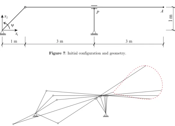
An interesting use for sliding joints is the modelling of mechanisms capable of describing some type of envisioned geometry, as cutting rocks or metallic sheets for civil or mechanical industries. Such mechanisms are commonly described in classical textbooks such as Shigley and Uicker (1981) and Norton (2011), among others, where analytical solutions for position analysis are presented. Usually, the numerical modelling of this kind of mechanism is done in a dynamic version. However, if the intention is to adjust the geometry to be described, a static position analysis should be better suit-ed, which is done in this example since no inertial forces are considered. Figure 7 depicts the initial configuration of a structure with a prismatic joint that connects a 6.0 m arm to a 1.0 m supporting bar. A prescribed rotation
is imposed on a crank that is connected to the main arm by a revo-lute joint. The rotation of the crank imposes a motion on the mechanism as depicted in figure 8.Figure 7: Initial configuration and geometry.
Figure 8: Selected configurations and arm free end trajectory.
Considering the restricted degrees of freedom and the boundary condition, this is an isostatic non-compliant linkage. Hence, only rigid boy motion takes place since nor strains or stresses are
1 m 3 m 3 m
1 m
1 x 2
x P
expected during the imposed quasi-static motion. Therefore, the dimensions and material properties of the involved bars may have any value. Although, in order to obtain a numerical solution, it is adopted for all elements square cross section with side 0.1 m, elastic modulus =2.0GPa and shear modulus =1.0GPa. Seventeen finite elements with cubic approximation are employed for discretization.
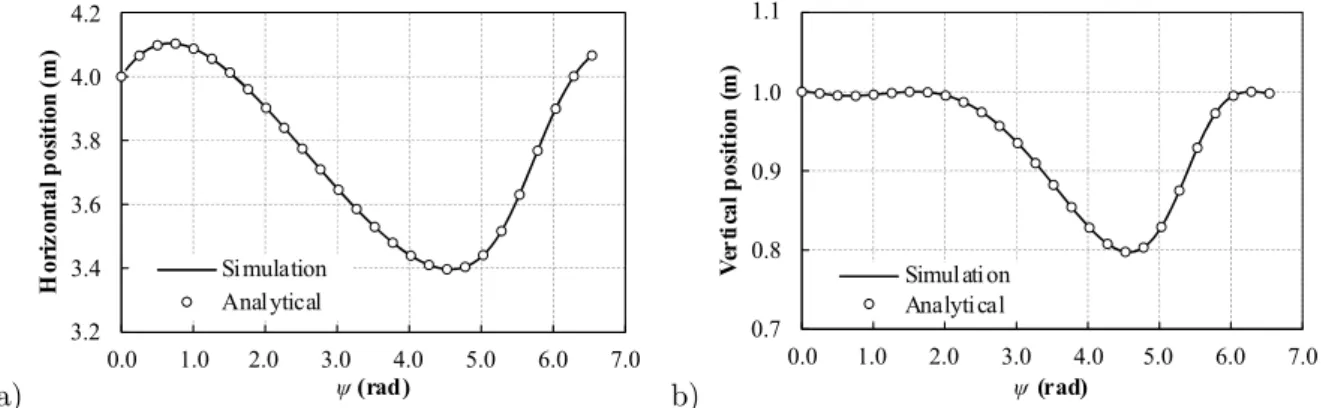
Figure 9 shows the arm free end trajectory (cutting geometry), point A, for a complete turn of the crank for the simulation and the analytical rigid body motion solution given by the referred textbooks. Also, the prismatic joint position, point P, evolution according to the prescribed rotation is compared with the analytical solution as shown in figure 10a and 10b for horizontal and vertical position, respectively.
Figure 9: Arm free end trajectory (point A).
a) b)
Figure 10: Prismatic joint position analysis (point P): a) horizontal and b) vertical position.
The motion was divided into 100 steps and less than six iterations are required for convergence in each step, see figure 11. Therefore, given the obtained results, one concludes that the presented formulation works very well and can be used for general analysis.
1.0 1.5 2.0 2.5 3.0
4.0 4.5 5.0 5.5 6.0 6.5 7.0 7.5
Ve
rt
ic
al
p
os
itio
n
(m
)
Horizontal position (m) Simulation
Analytical
3.4 3.6 3.8 4.0 4.2
0.0 1.0 2.0 3.0 4.0 5.0 6.0 7.0
H
or
iz
on
tal
p
os
iti
on
(m
)
ψ(rad) Simulation Analytical
0.8 0.9 1.0 1.1
0.0 1.0 2.0 3.0 4.0 5.0 6.0 7.0
Ve
rt
ic
al
p
os
itio
n
(m
)
Figure 11: Evolution of the number of iterations for solution.
7.2 Doubly Bent Beams with Bifurcation
Since in the last example finite deformations are present only due to rigid body motion, here we present an interesting example of bifurcation of equilibrium under traction that shows large dis-placements and rotations in a deformable structure involving sliding connections.
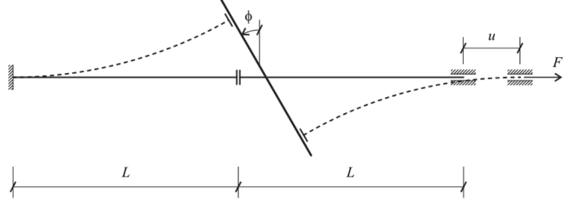
Figure 12 presents two flexible bars with length L=0.25 m that are initially aligned and to which is imposed a horizontal displacement u. The reactive traction force F in the right support is also measured. Those bars are connected by prismatic joints to a rigid bar long enough to allow large deformations on the structure. Here the rigid bar length is adopted as 10.0 m.
Figure 12: Initial and deformed configurations of the structure.
Analytical solution and experimental validation of this phenomenon were presented by Zaccaria et. al. (2011). For the numerical simulation, a rectangular cross section is adopted to both flexible bars with h0 =1.0 mm and b0 =25.0 mm. For the rigid bar a squared 1.0 m side cross section is chose. Each of the three bars were modelled by four cubic finite elements with the same material properties: =200.0GPa and =100.0 GPa.
In order to find the non-trivial solution, a perturbation is introduced to the system as an initial inclination of the rigid bar by an angle f0. Increasingly smaller values for the initial angle were adopted to show convergence to the analytical solution. The results for the rigid bar rotation f,
5 6 7
0.0 1.0 2.0 3.0 4.0 5.0 6.0 7.0
Nu
m
be
r
of
it
er
at
io
ns
ψ(rad)
u
F
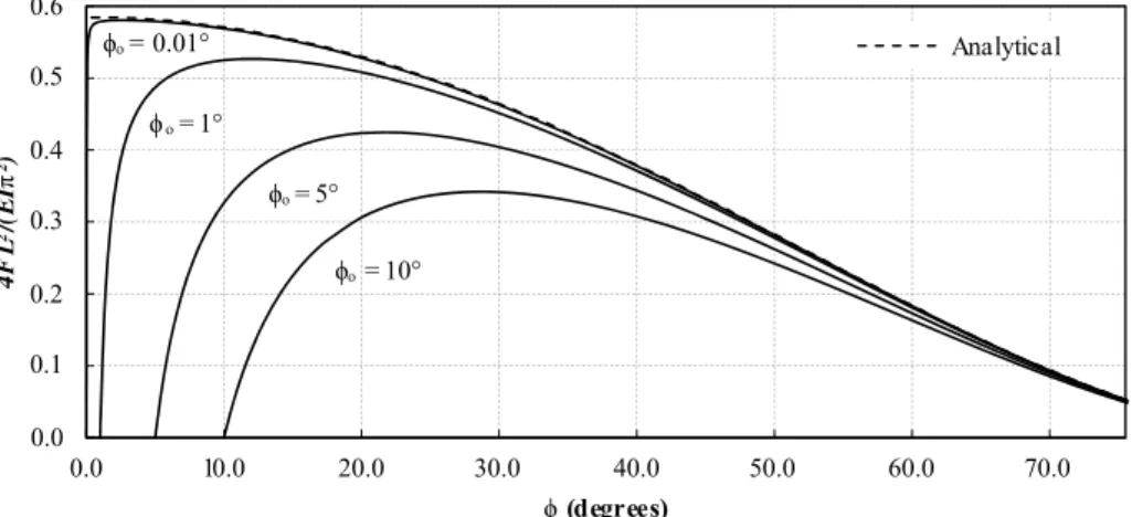
Figure 13, and right support horizontal displacement, Figure 14, against a non-dimensional traction force 4FL2 /Ip2, where
I
is the second area inertia moment, shows the efficiency of the formula-tion when handling geometrical nonlinear problems.Figure 13: Rigid bar rotation angle.
Figure 14: Right support horizontal displacement.
Figure 15: Evolution of the number of iterations for solution.
0.1 0.2 0.3 0.4 0.5 0.6
0.0 10.0 20.0 30.0 40.0 50.0 60.0 70.0
4F
L
2/(
E
I
π
2)
ϕ(degrees)
Analytical
ϕₒ = 10° ϕₒ = 5° ϕₒ = 1°
ϕₒ = 0.01°
0.1 0.2 0.3 0.4 0.5 0.6
0.0 0.2 0.4 0.6 0.8 1.0 1.2 1.4 1.6 1.8 2.0
4F
L
2/(
EI
π
2)
u/2L
Analytical ϕₒ = 0.01°
ϕₒ = 10° ϕₒ = 5°
ϕₒ = 1°
10 20 30 40
0.0 0.5 1.0 1.5 2.0
N
um
ber
o
f i
ter
at
io
ns
u/ 2L
The horizontal displacement was imposed in 200 steps and the mean number of iterations re-quired for solution was 13 for each step. Figure 15 presents the evolution of the number of iterations for the extreme cases of the initial inclination angle since the other results have a similar pattern. Only in the first step of the smallest initial angle several iterations were needed. This is expected since the strong deformation of the structure that occurs in this particular step is due to the bifur-cation of equilibrium.
7.3 Influence Lines of a Bridge - Moving Load
This example is presented in order to demonstrate the capabilities of the proposed sliding joint for-mulation to determine influence lines at any cross section for general structures. One important information about influence lines and internal efforts envelope for non-linear applications is that the superposition principle is not valid and exhaustive calculations are performed. However, when small displacements take place the superposition of results is recovered.
Particularly in this example, the influence lines of internal efforts at the central cross section (point P) of a bridge subjected to a load train is calculated, see figure 16. The vehicle is modelled by a frame with 4.0 m length and 1.0 m high. The contact between the vehicle and the bridge is modelled by two cylindrical joints allowing their relative movement. A vertical 15 kN load is ap-plied on the mid-span of the moving frame and a displacementu =26.0 m (divided into 500 steps) is imposed at its left corner. Figure 16 depicts the geometry of the bridge and the vehicle for the initial configuration.
A rectangular cross section with width b0 =1.0 m and height h0 =2.0 m is adopted for the bridge, and a square cross section with side a =0.1m is adopted for the vehicle. The bridge elastic and shear modulus adopted are =20.0GPa and =10.0GPa, respectively. For the vehicle, the material properties are 10 times greater. Six finite elements with cubic approximation were used to model the frame representing the vehicle and 34 elements for the bridge. Since the objective is to evaluate internal efforts, two finite elements with 1.0 mm each are placed on both sides of point P to avoid the passage of any concentrated load on its domain. This is necessary due to the disconti-nuity of internal efforts and the contidisconti-nuity of shape functions, inherent to finite elements.
Figure 16: Vehicle initial configuration and geometry.
Figure 17 presents the vertical displacement influence line at the bridge mid-span (point P). As expected, the greatest displacement of -0.55 mm occurs when the load train is centralized with the bridge beam. Influence lines for the bending moment and shear force are shown in figures 18
5kN
1
x
2
x
P u
1 m
and 19, respectively. As expected, the maximum efforts occur when one of the cylindrical joints (wheel) are placed over point P.
In the solution process every step needed exactly 10 iterations for convergence. As one can see, results are quite accurate and no limits for the bridge vertical geometry or number of wheels are present for the proposed formulation, revealing the versatility of the technique for practical applica-tions.
Figure 17: Bridge mid-span displacement influence line.
Figure 18: Bridge mid-span bending moment influence line.
Figure 19: Bridge mid-span shear force influence line.
-0.06 -0.05 -0.04 -0.03 -0.02 -0.01 0.00 0.01
3.0 5.0 7.0 9.0 11.0 13.0 15.0 17.0 19.0 21.0 23.0 25.0 27.0 29.0
V
ertical
dis
pl
acem
ent
(m
m
)
Load point horizontal position (m)
-30.0 -25.0 -20.0 -15.0 -10.0 -5.0 0.0 5.0
3.0 5.0 7.0 9.0 11.0 13.0 15.0 17.0 19.0 21.0 23.0 25.0 27.0 29.0
Bend
in
g
m
om
ent
(k
N
.m
)
Load point horizontal position (m)
-8.0 -6.0 -4.0 -2.0 0.0 2.0 4.0 6.0 8.0
3.0 5.0 7.0 9.0 11.0 13.0 15.0 17.0 19.0 21.0 23.0 25.0 27.0 29.0
Sh
ea
r fo
rce
(k
N
)
7.4 Equilibrium Path of a Shallow Arch with Crank
A shallow arch with its motion enforced by a crank is present in this example. The arch is fixed by simple supports that allow rotation but not translations. The arc has a span of L=10.0 m and height of h =1.0 m. The crank is subjected to a rotation of
=1.8 rad divided into 500 equal steps. The connection between the crank and the arch is made by means of a cylindrical joint, as depicted in figure 20. In the initial configuration the dimensions indicated in figure 20 are:2.4606 m
H = , d1 =1.6178 m andd2 =0.5523 m.
All structural components are flexible and have square cross section with side a=10.0 cm. Twelve finite elements with cubic approximation were used to model the arch, which has an elastic modulus of =200.0 GPa. The crank is modelled by five finite elements and has elastic modulus ten times greater than the arch. The shear modulus for all components is adopted as half of the elastic modulus.
Figure 20: Structure initial configuration.
The evolution of the reaction moment required to move the fixed end of the crank is presented in figure 21a along with some deformed configurations of the system. The evolution of the normal force at the crank is presented in figure 21b. The arch mid-span vertical position is depicted in fig-ure 21c. One can observe from those curves the occurrence of instabilities by limit points, indicated by the change of sign for the crank normal force and bending moment. At these positions the arch assumes an indifferent equilibrium configuration.
Furthermore, from the discontinuity of the curves achieved at a rotation of
=1.656 rad it is clear the existence of the snap-back phenomenon. However, as it is known, it is not possible to de-scribe the equilibrium path at back situations using the Newton-Raphson method. The snap-back is present because the driven unstable shape is not a controlled one.In order to describe this portion of the curve it would be necessary the use of an arc-length type method for the solution of the system that is beyond the objectives of this study.
Each step required at most 5 iterations to converge as shown in figure 22. Only in the step that the snap-back occurred several iterations were needed. However, it is expected due to the large change of configuration of the arch at this point of the analysis.
x
2
x
2
d
1
d H
h
Therefore, from results, the potentialities of the proposed formulation and its consistency on evaluating structural behaviour are evident.
Figure 21: Equilibrium path: a) reactive bending moment and structure configurations, b) crank mid-point normal force, c) arch mid-span vertical position.
Figure 22: Evolution of the number of iterations for solution.
-150.0 -100.0-50.0 0.0 50.0 100.0 150.0
200.00.0 0.2 0.4 0.6 0.8 1.0 1.2 1.4 1.6 1.8
No
rm
al
fo
rc
e (
kN
)
(rad)
-1.5 -1.0 -0.5 0.0 0.5 1.0
1.50.0 0.2 0.4 0.6 0.8 1.0 1.2 1.4 1.6 1.8
Ve
rt
ic
al
po
si
ot
io
n (
m
)
(rad)
-600.0 -400.0 -200.00.0 200.0 400.0 600.0 800.0
1,000.00.0 0.2 0.4 0.6 0.8 1.0 1.2 1.4 1.6 1.8
Be
nd
in
g
m
om
en
t(k
N
.m
)
(rad)
a)
b)
c)
10 20 30 40
0.0 0.3 0.6 0.9 1.2 1.5 1.8
Nu
m
be
r
of
it
er
at
io
ns