Abstract
A combination of vectorial form of wave method (VWM) with Fourier expansion series is proposed as a new vehicle for free and forced vibration analysis of stepped cylindrical shells with multiple intermediate flexible supports. The flexible supports can include springs with arbitrary properties in the possible directions. Based on Flügge thin shell theory and VWM, the reflection, propagation, and transmission matrices for a circular cylindrical shell are de-fined. Furthermore, contiguous vector-matrix relationships are established for free and forced vibration analysis of the issue in-cluding an arbitrary number of the discontinuities in the shell thickness, or shell steps, and intermediate supports. Using these vector-matrix relations, the equations of motion as well as the system continuity are well satisfied. Dimension of these vectors and matrices are completely, independent of the number of the applied supports and geometrical steps in the shell. Hence, the present approach provides excellent computational advantages and modeling flexibility compared to the conventional vibration analy-sis methods available in the literature. The results of the present study are compared with the results available in the literature as well as the results of finite element method (FEM) and found in excellence agreement. Furthermore, as a case study case, a cylin-drical shell with three flexible intermediate supports and also three geometrical steps is considered. The natural frequency and mode shapes of the issue are derived, and the forced responses of the shell subject to point load excitation are reported.
Keywords
Intermediate flexible supports; stepped cylindrical shell; extended vectorial-wave method; free and forced vibration.
Free and Forced Vibration Analysis of Stepped Circular
Cylindrical Shells with Several Intermediate Supports Using
an Extended Wave Method; a Generalized Approach
Reza Poultangari a
Mansour Nikkhah-Bahrami a, b, *
a Department of Mechanical and
Aero-space Engineering, Science and Research Branch, Islamic Azad University, Teh-ran, Iran; 14515-775.
b School of Mechanical Engineering,
College of Engineering, University of Tehran, Iran; 14395-515
http://dx.doi.org/10.1590/1679-78252876
1 INTRODUCTION
Using intermediate supports for long pipe uniform or non-uniform shells in many industries is a com-mon way for protecting the system from the occurrence of resonance failure and improving the sys-tem robustness. In this regard, rigidity consideration for the supports applied, called classical sup-ports, is an over simplified assumption bring significant deviations between the theoretical and exper-imental results. It is clear that as much as the characteristics of non-rigid supports can play a great rule on variation of the responses of the whole vibrating system. In addition, existence of discontinui-ty in the shell thickness or shell steps is inevitable in many industrial elements such as accumulators, fluid tanks and pipes. Hence, following the importance of the support characteristics and the non-uniform thickness of the shell in the practical application, the researchers have been encouraged to examine these effects on the vibration analysis of shells like in Zhou et al. (2012), Qu et al. (2013), Chen et al. (2015), Chen et al. (2013), and finally Wang et al. (1997). In this way, different numerical methods, e.g. finite element method (FEM) like in Salahifar and Mohareb (2012), weighted residual method as in Qu et al. (2013), generalized differential quadrature method (GDQ) as in Loy et al. (1997), and analytical solutions, e.g. close form solutions as those represented by Chen et al. (2013), wave based method (WBM) like in Chen et al. (2015), transfer function method (TFM) as in Zhou et al. (1995) and state space techniques (SST) like in Zhang and Xiang (2007), are proposed for analysis of such systems.
Analytical modeling of vibrations of uniform shells with interior supports has been a critical issue in the recent analytical studies, perhaps due to requirement of satisfying the continuity and the sup-port conditions simultaneously, like in Qatu (2002), Xiang et al. (2002), Zhang and Xiang (2006) and Loy and Lam (1997). Hence, a few researches been conducted in this area, and their proposed meth-ods are numerated and contain several limitations. For example Xiang et al. (2002) solved the issue of free vibrations of a uniform shell with several intermediate ring-, or radial rigid-supports. They pro-posed a state-space technique combined with domain decomposition method in order to satisfy conti-nuity as well as support conditions of the issue. In this direction, Zhang and Xiang (2006) with the same methodology proposed in Xiang et al. (2002), solved the problem of free vibrations of a uniform open shell with multiple intermediate Ring Supports (RS). Although the results of the method pro-posed in Xiang et al. (2002) are promising as an analytical method, the applied intermediate RS were not flexible and were only limited in the one direction, i.e. radial direction. The vibration analysis of stepped shells and modeling of the flexible supports are possible using the numerical methods, e.g. FEM where proposed in Qu et al. (2013). However, solving the problem demands several degrees of freedom for the issue and accordingly extensive memory resources and high computational resources (this important evaluated in Qu et al. (2013)). Moreover, in special applications such as designing with optimization, systems controls, inverse problems, and real time applications, accurate and fast system responses as well as low system memory are required simultaneously. Thus, in the mentioned applications, applying the conventional and efficient numerical methods like FEM may fail to capture the shell response within a reasonable computational time and accuracy.
provid-ing robust, fast, and accurate results for vibration analysis of shells, is highly demanded to deal with the design problems with less limitations and more capabilities.
Vectorial wave method (VWM) is a well-known method, which was first introduced by Mace (1984) and applied to free and forced vibration analysis in straight beams. Thereafter, VWM was applied in vibration analysis of several wave guide elements such as bars, Hagedorn and Das-Gupta (2007), straight-,Mase (2005), and curved-beams and frames in two,Lee et al. (2007), or three dimen-sions, Mei (2016), rings, Huang et al. (2013), plates, Ma et al. (2015) and Renno and Mace (2011), and membranes, Bahrami et al. (2012). However, this method has not been extended for other me-chanical elements such as shell like geometries.
Review of the literature shows that there have been few attempts for extension of VWM to more complex issues such as existence of multiple geometrical steps or multiple intermediate supports in considered geometry. Nikkhah-Bahrami et al. (2011) have proposed a modified form of VWM for free vibration analysis of non-uniform mechanical elements (beams) with arbitrary numbers of discontinu-ities. They demonstrated that by distinctive combinations of VWM matrices and their inversions, it is possible to provide a reduced order vector-matrix relationship, independent of number of disconti-nuity of the considered issue. However, due to singularity of the reflection and transmission matrices in the vicinity of rigid intermediate supports, the proposed method in Nikkhah-Bahrami et al. (2011), cannot be extended to the issues with intermediate supports. To the authors’ best knowledge which is supported by a critical literature survey, the VWM has not yet been utilized for vibration analysis of shell elements or problems with interior supports perhabs due to lack of establishment of proper wave vectors and relevant matrices.
The present study aims to extend VWM method to the case of stepped cylindrical shell elements with interior flexible supports, as barriers in the direction of the wave dispersion. Hence, proper wave vectors and relevant matrices relationships for these kinds of wave barrier are stablished. By intro-ducing a canonical relationship between carrier waves and the displacement field, a general case study including possible barriers in the path of wave motion, flexible intermediate support types and geometrical steps, are considered. Base on carrier wave vector motion in each shell segment and communication between the waves in all the shell interfaces, extended VWM is utilized for free and forced vibration analysis of cylindrical shells with discontinuities in their thickness in the presence of several intermediate flexible supports.
2 GOVERNING EQUATIONS
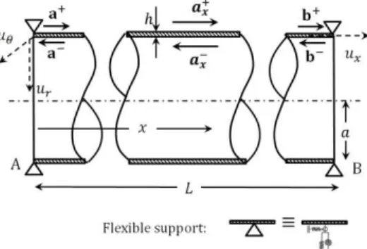
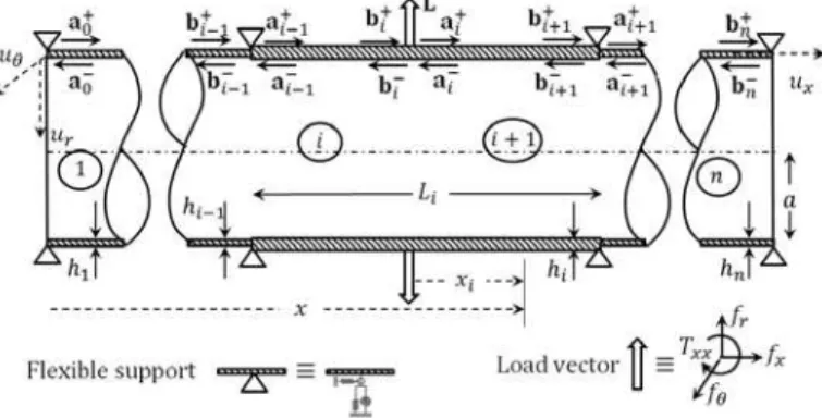
Figure 1 shows a cylindrical shell with the length L, thickness h, Poisson ratio , Young's modulus E, density ρ and middle layer radius a. The governing equations of motion based on Flügge theory for a cylindrical shell as demonstrated in Figure 1 can be expressed as follows:
0
33 23 13
23 22 12
13 12 11
r
x
u u u
L L L
L L L
L L L
(1)
where, Lij (i,j=1,2,3) are differential operators as shown in appendix A. Furthermore, ux, ,r are the
direc-tions, respectively. Using time harmonic functions and complex Fourier expansion in the circumferen-tial direction, as to satisfy Eq. (1), the displacement fields can be represented in the respective direc-tions as:
Figure 1: Wave’s motion in a homogeneous cylindrical shell with flexible ended supports.
n
ωt n x r
n
ωt n x
n
ωt n x
x C u αC u C
u ei( ), ei( ), ei( ) (2)
where, C is a constant;
and
are displacement ratios, which are respectively introduced as α=uθ /ux and β=ur/ux. In Eq. (2), is the wave number, n is the circumferential mode number (or integerconstant of the Fourier terms) and ω is circular frequency. In fact, Eq. (2) consists of the displace-ment field regarding to all possible real and imaginary excitation responses of the shell. To obtain real parts of the calculated results, a half-range expansions of the Fourier series is enough for the issue, i.e. n=0 to ∞. To establish the parameters of and ω, Eq. (2) is substituted in the equation of motion, Eq. (1), which yields:
0 1
4 33 2 33 33 33 23
13
2 23 23 23 2
22 22 22 12
12
3 13 13 13 12
12 2
11 11
C E
C A
C A C
A B
D B B
A
(3)
where Λ is a dimensionless wave number as Λ= a, and χij (i,j=1,2,3) are the matrix elements. The
expressions (A,B,C,D)ij (i,j=1,2,3) are given in Appendix B. To achieve the non-trivial results and
hence the non-zero displacement fields, the determinant of the coefficients matrix in Eq. (3) should be equal to zero, i.e. | χij |=0.
By defining a dimensionless frequency Ω=ωa((1- 2)ρ/E)0.5 (or frequency factor) as the matrix square eigenvalues [ χij], we can achieve a logical relationship among the dimensionless wave numbers
Λ and frequency factor Ω with the aid of | χij |=0. These relations are established for all kind of
ve-locities of wave’s dispersion in the shell, i.e. the phase velocity and the group velocity of the waves (Lee et al. (2007) and Karczub (2006)) where this issue will not be discussed here. Mathematically, |χij |=0 leads to a polynomial of degree four in terms of square of dimensionless wave number Λ2 as
follow:
0
0 2 2 4 4 6 6 8
8Λ A Λ A Λ A Λ A
in which Ai (i=0,2,4,6,8) are five coefficients represented in the appendix C. The eight possible roots
of Eq. (4) are analytically derived and discussed in appendix D. According to the wave theory, dis-placement fields, Eq. (2), can be expressed in the form of
n ωt r x r x U
u,, ,,ei where expressions of Ux,,r can be described as linear combinations of eight harmonic functions in the x, and r directions as follows:
nj x j j j x j j r n j x j j j x j j n j x j j x j x a a x U a α a α x U a a x U i 8 5 i-4 1 i i 8 5 i-4 1 i i 8 5 -i 4 1 i e ) e e ( , e ) e e ( , e ) e e ( ,
(5)where, expressions j
a andaj(j1 ,...,8) are the positive and negative going wave amplitudes of kind of
carrier waves where in fact, they are carring Lamb waves in the axial direction of the shell. These wave amplitudes show the contribution of each corresponding wave in the displacement fields of the vibrating shell. These waves can be of kind of pure harmonic (or propagating waves), or harmonic-damping (or standing waves) or pure harmonic-damping (or evanescent waves) waves depending on the corre-sponding wave number values (see appendix D). For the above composition, based on the conjuga-tion of roots of Eq. (4), the wave numbers are arranged as mm4 , m0 where m1 ,...,4.
3 MATRICES OF WAVE MOTION
3.1 Force and Displacement Vectors
For free vibration analysis of a cylindrical shell via VWM, the vectors of positive and negative going waves, governing the problem, are required to be defined. Thus, the following form is considered for wave amplitudes: ) ( ) ( ) 8 ( 4 ) 7 ( 3 ) 6 ( 2 ) 5 ( 1 i i i i ) ( ) ( e 0 0 0 0 e 0 0 0 0 e 0 0 0 0 e ) ( ) 8 ( 4 ) 7 ( 3 ) 6 ( 2 ) 5 ( 1 a F a x a a a a x x x x x x (6)
where, Fare propagation matrices, aare vectors of wave amplitudes and
x
a are waves vectors, that are all going in the right (+) or left (-) directions along with shell axis as depicted in Figure 1. By defining the vectors of amplitudes w and f for the displacement vector (w) and the force vector (f) both vectors of w and f are considered as follows:
nxr x xx xx n n r r x n V T M N x x U U x U U x x i T i i T i e e ) ( ) , ( e e ) ( ) , ( f f w w (7)
parameters which are introduced in the Appendix E. In Eq. (7), prime symbol (') indicates that the term is divided by exp(it).
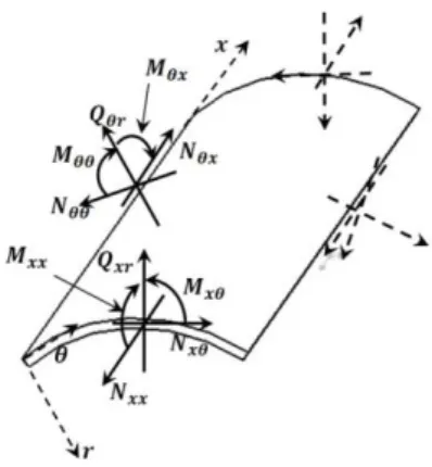
Figure 2: Force and moment resultants in a circular cylindrical shell.
To consider the impact of structural damping in cylindrical shell, the Young's modulus is adopted as EEˆ(1i ), where γ is the structural loss factor and Eˆ is a real coefficient of Young's modulus related to the material used in the cylinder.
3.2 Definition of Matrices ψ and φ
By defining certain interface metrics, it is possible to express the displacement and force vectors by the positive and negative going wave vectors, respectively. Hence, by substituting Eqs. (5) in Eq. (7) yields following relationship:
) ( , ) ( x x x x x
x ψ a ψ a f a a
w (8)
where, ψand are matrices of displacement vectors and force vectors, respectively. These relations
can be written as follows:
] [ ] [ ) 8 ( 4 ) 7 ( 3 ) 6 ( 2 ) 5 ( 1 ) ( ) 8 ( 4 ) 7 ( 3 ) 6 ( 2 ) 5 ( 1 ) (
ψ ψ ψ ψ
ψ
(9)
where, vectors of φj and ψj (j=1,…,8) as elements of ψ and , as follows:
in which kEh( 1 2)1 and DEh3( 12(1 2))1 are respectively membrane and bending stiffness of the shell. The relation between propagating wave vectors within the shell, e.g. aand bor band ain
the Figure 1, are made by the propagation matrices. The propagation matrix elements in the positive and negative direction, F, can be determined by the following relation:
... ,
,
,
11 11 11 11 11
11
a b F a b F
b F a a F
b (11)
where, F, introduced in Eq. (6), shows the propagation matrices in a cylinder with the length of x=L.
3.3 Definition of Reflection and Transmission Matrices
Taking into account the effects of flexible supports on the vibrations of cylindrical shell, it is neces-sary to define the stiffness matrix. This matrix in location is defined as follows:
r r
x
K K K K
0 0 0
0 0
0
0 0 0
0 0 0
K (12)
The diagonal elements (K)(x,r,,r)are the stiffness coefficients of springs which are extended evenly in arbitrary position on the cylinder. The diagonal shape of the matrix in Eq. (12) is appropriate for the linear vibration analysis of continuous systems, such as cylindrical shells.
3.3.1 Ended Supports
The boundary conditions at the right and left supports, depicted in the Figure 1, should be satisfied. In order to satisfy these boundary conditions one can write:
fKw
A,B (13)According to Figure 1, the vectors of the incident wave amplitudes in the left and right bounda-ries are a and b, respectively. Moreover, the reflected waves vectors at these two boundaries are a
and b, respectively. Now the reflection matrix is constructed by Eqs. (8) and (13). In this regard,
these equations were set based on the incident (a, b) and reflected waves (a, b) vectors as
fol-lows:
R a
a A , b RBb (14)
where, RA,Bare reflection matrices at the left and right borders of cylindrical shell, which can be de-fined by the following equations:
) (
) (
), (
)
( A 1 A B B 1 B
A K K R K K
It is clear that the set of equations of RAand RB in Eqs. (15) can satisfy the flexible boundary conditions for the both ends of the cylinder.
3.3.2 Wave Motion in Vicinity of Intermediate Supports and Shell Steps
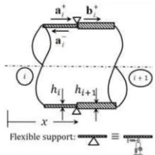
In the analytical and semi-analytical solutions provided for the free vibrations of cylindrical shells, rarely can we find references on the flexible intermediate supports in the literature. The present sub section is intended to consider the effect of interior supports and shell steps on the vibration analysis of the cylindrical shell. Hence, Figure 3 shows incidence of a wave with a barrier including of a flexi-ble support and a shell step.
Figure 3: Waves motion in the vicinity of intermediate wave barriers of kind of shell step
and intermediate support at same position
As seen in Figure 3, a part of the incident wave vector
i
a after colliding with the barrier is trans-ferred
i
b , and some of it will be reflected i
a . Thus, considering the continuity conditions and the balance of forces in the barrier between the ith and the (i+1)th segments of the shell, we have:
0 ) 1 or ( 1
0
1 , - ( )
i x i i m i i i x
i w f f K w
w (16)
in which (Km)i is the rigidity matrix of the ith intermediate support of the ith barrier that is a diago-nal matrix including of elements of spring stiffness coefficients in the relevant independent directions, i.e. x, r , and r in Eq. (12). Using Eq. (8) in Eq. (16), and according to the equality of geometric and mechanical properties of the cylindrical shell in each segment, the following equality is concluded:
i i i m i
i i i i i
i i i i i i
b K b a a
b ψ a ψ a ψ
1 1
1
)
(
(17)
Reflection and transmission matrices that connect the incident wave vector to the barrier,
i
a ,
transmitted vector,
i
b , and reflected vector,
i
a , are defined as follows:
i i i i i i i
i t a a r a
b , 1 , 1, (18)
the results of Eq. (18) and rearranging Eq. (17), the reflection and transmission matrices can be ob-tained as: ) ( ] [ ) ] )[ ) ( ( ( ) ] )[ ) ( ( ( , 1 1 1 1 , 1 1 1 1 1 1 1 1 1 , 1 i i i i i i i i i i i m i i i i i i m i i i i r t K K r (19)
where, I is a four by four identity matrix. In a same manner, the reflection and transmission matrices in the opposite direction, i.e. right to left direction, can also be obtained.
4 EXTENDED VECTORIAL WAVE METHOD
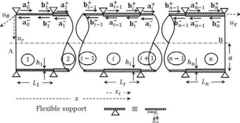
In Figure 4, wave motion in a cylindrical shell with several elastic supports is shown. Accordingly, the relationship between the vectors of the output waves from the first intermediate support, i.e.
1
b
and
1
a , in terms of input waves vector to the support i.e.
1
b and
1
a , is as follows (it should be noted that for homogeneous materials like the present issue we have F F F):
Figure 4: Waves motion in the vicinity of intermediate barriers of kind of intermediate supports and shell steps.
1 1 , 2 1 1 , 2 1 1 2 , 1 1 2 , 1 1 0 1
1 F( )a , a t b r a , b t a r b
b L (20)
Moreover, by considering
0 A 0 R a
a and
1 1 0 F( )b
a L and using Eq. (20), we can write:
1 1 1 a a (21)
where,
1, as a positive going inductor matrix, is defined as follows:
2 , 1 1 , 2 1 A 1 1 1 , 2 1 A 1 2 , 1
1 t (IF( )R F( )r ) F( )R F( )t r
L L L L
(22)
In a same manner, the following relation can be given between
i
a and
i
a for the ith intermediate support, i=2…n-1, as:
1 ,..., 1 ..., , 2 2 2 n i i i i a a a
a
where, the same as those given in Eq. (24),
2 to n1 are defined as:
1 ,..., 2 ) ( ) ( ) ) ( ) ( ( ... ) ( ) ( ) ) ( ) ( ( 1 , , 1 1 1 , 1 1 1 , 3 , 2 2 , 3 2 1 2 1 2 , 3 2 1 2 3 , 2 2 n i L L L L L L L L i i i i i i i i i i i i i i
i t I F F r F F t r
r t F F r F F I t (24)
Finally, in the nth segment of the shell, the following relations are established:
1 1 1 1 B
1, , ( ) ,
)
( n n n n n n n n n n
n F L a b R b a FL b a a
b (25)
The above equations consist of four equations with for unknown vectors, namely 1
n a ,
1
n
a ,
n b , and
n
b . Obviously, we can solve the sets of Eqs. (25) by each of these unknowns. For example, Eq. (25) can be solved by
n
b as follows:
0 b R F F
I
n n
n
n L
L ) ( ) )
(
( 1 B (26)
To achieve a non-trivial solution for free vibration analysis of the issue, using Eq. (26), the de-terminant of the coefficient of
n
b should be equal by zero. It should be noted that Eq. (26) is not a unique way for calculating the natural frequencies of the shell and we are able to write the same rela-tions by the other wave vectors depicted in Figure 4. For example, in a backward approach, for the waves that are moving in the vicinity of the (n-1)th intermediated support (or the last intermediate support) of the shell, we have:
1 n1,n n1 n1,n n, n1 n,n1 n1 n,n1 n1
n t b r a b t a r b
a (27)
Furthermore, in the nth segment or the last segment of the shell, we can write:
n n n n n
n F L a a F L b
b ( ) 1, 1 ( ) (28)
considering
n n R b
b B and using Eq. (27) and (28), it gives a relation between bn1and
1
n
b as follows:
1 n1 n1
n Γ b
b (29)
where, 1
n
Γ is a negative going inductor matrix, which is defined as:
1 , , 1 B , 1 B 1 ,
1 ( ( ) ( ) ) ( ) ( )
nn n n n n n n n n nn n t I F L R F L r F L R F L t r
Γ (30)
It is possible to obtain a general relationship between i
b and i
b for the ith intermediate support,
i= 1, …, n-2 as follows:
1 ,..., 1 ..., , 2 2 2 n i i i i n n
n Γ b b Γ b
b
(31)
where,
1
Γ to 2
n
1 ,..., 2 ) ( ) ( ) ) ( ) ( ( ... ) ( ) ( ) ) ( ) ( ( , 1 1 , 1 1 1 , 1 1 1 , 1 2 , 1 1 , 2 1 2 1 1 , 2 1 1 1 2 , 1 2 n i L L L L L L L L i i i i i i i i i i i i i i i n n n n n n n n n n n n n n n r t F Γ F r F Γ F I t Γ r t F Γ F r F Γ F I t Γ (32)
Wave motion in the first shell segment where depicted in the Figure 4 is considered here. By con-sidering the canonical relationships between these wave vectors the following relations are governed:
1 1 1 1 1 0 0 A 0 0 1
1 F( )a , a R a , a F( )b , b b
b L L (33)
The above set of equations consist of four equations with four unknowns, i.e.
0
a ,
a
0, 1
b and
1
b . For example, solving the above set of equations by
0
a gives the following relation:
0 a R F Γ F
I
0 A 1 1
1) ( ) )
(
( L L (34)
For non-trivial results in the above equation, the determinant of the coefficient matrix of
a
0must be zero, so we have:0 R F F
I
A 1 1
1) ( )
(L L (35)
Invoking Eq. (35), all of the natural frequencies can be determined for a stepped shell with sever-al intermediate supports with individusever-al arbitrary properties for the applied supports. It is interesting to notice that both determinations represented in Eq. (26) or (35) provide a unique result for the frequency analysis of the shell. To achieve the roots of Eq. (35), Wittrick-Williams stemming algo-rithm can be used (Lee et al. (2007)). In addition, by normalizing the wave vector
0
a and setting it from Eq. (34) in terms of the natural frequencies of the system, the mode shapes can be obtained.
5 FORCED VIBRATION
Figure 5: Waves motion in the vicinity of loading position.
As a general case, it is possible to choose any arbitrary function, including concentration point loading, in the circumferential direction using Fourier expansions. Effects of the ring harmonic load-ing on structural responses of the shell, can be obtained usload-ing the wave motion analysis within the shell in the vicinity of the loading position. Continuity and force balancing between ith and (i+1)th segments of the shell exactly at the loading position are satisfied by the following relations:
t t x i i x t i t i
i i
0 1 0
i 1
i e , ( - ) e e
e w f f L
w (36)
where, indices i and i+1 in the above equation are referred to the left and right sides of the loading positions, respectively. Furthermore, L is the ring loading vector consists of force and moment load-ing in the relevant directions as follows:
Tr xx
x T f f
f ( ) ( ) ( ) ( )
L (37)
where, fx,,r and Txx, are distributed forces and torque in the related directions, respectively. Substi-tuting Eq. (8) in Eq. (36), it gives:
L a a b b a a b b ) ( )
( i i i i i i i i i i i i i i i i (38)
or in the vector-matrix form it can be written as:
L 0 a b a b i i i i i i i i (39)
where, i
a and
i
b are the opposite going wave vector amplitudes at both sides of loading position, Figure 5. Solving the above equation yields:
Π Π L Π Π a b Π a b i i i i i i i i i i
( )1 )1 , ( )1
( , , (40)
From the wave motion analysis in the both sides of the loading position we can find:
i i i i i
i b a a
where, matrices of iand i1 are defined as:
) ( ) (
), ( )
( 1 1 1 1 1
i F Li i F Li i F Li i F Li (42)
By eliminating i
b and i
a from Eqs. (40) and (41) we can write:
Π a b
Π I
a
i i i
i i i i
i i
1
1 1
1) (( ) )
(
(43)
Accordingly, for a certain load vector with arbitrary functions of , i
a and i
b can be calculated from Eq. (43). Using Fourier expansion, arbitrary functions of can be provided for load vector, L. Accordingly we can use of the following relation:
n n n T
r xx
x T f f
f ( ) ( ) ( ) ( ) Lei
L (44)
where, Lnis vector of Fourier parameters, and it can be obtained as follows:
f T f f T n d
r xx
x n
i
e ) ( ) ( ) ( ) ( 2
1
L (45)
For modeling the point load excitation in arbitrary position on the shell, e.g. x=0 and 0, in Figure 5, the point load can be expressed in terms of Dirac delta function:
n
n n T
r xx
x
x f T f f
i 0
0 ( ) L e
L
(46)where,
f
x,,r and Txx, are amplitudes of distributed forces and torque in the relevant directions,re-spectively. Hence the Fourier coefficient parameters in the presence of point loading,
L
n, can be obtained as follows:
0 0 0 0
i 0i 0
e 2
1
e ) ( 2
1
n T r xx
x
n T
r xx
x n
f f T f a
ad f
f T f
a
L
(47)
In the above equation,
f
x0, ,r and 0xx
T , are the point forces and concentrated torques at 0,
engineer-ing accuracy. Usengineer-ing Eqs. (7), (8) and (10) and wave amplitudes obtained from Eq. (43), i.e. i a and
i
b , for arbitrary distance, x, in the left or right sides of loading position, the amplitudes of the dis-placement fields in x, or r directions are obtained from the following relations:
i i i i i r i i i i i r i i i i i i i i i i i i i i i x i i i i i x x x U x x U x x U x x U x x U x x U a F a F b F b F a F a F b F b F a F a F b F b F ) ( ] , , , [ ) ( ] , , , [ ) ( ] , , , [ ) ( ] , , , [ ) ( ] α , α , α , α [ ) ( ] α , α , α , α [ ) ( ] α , α , α , α [ ) ( ] α , α , α , α [ ) ) ( ) ( ]( 1, 1, 1, 1 [ ) ) ( ) ( ]( 1, 1, 1, 1 [ 8 7 6 5 4 3 2 1 1 , 8 7 6 5 4 3 2 1 , 8 7 6 5 4 3 2 1 1 , 8 7 6 5 4 3 2 1 , 1 , , (48)
Accordingly, using Eqs. (43) and (48), all of displacement responses for the ith and (i+1)th seg-ments of the shell can be obtained for arbitrary positions on ith and (i+1)th segments of the shell. In a same manner and by using Eqs. (23) and (31), similar relationships for the other segments of the shell can be founded easily.
6 NUMERICAL RESULTS
In this section, free and forced vibrations of stepped circular cylindrical shells affected by their sup-ports characteristics, will be examined using the defined vector-matrix relations of VWM in the pvious sections. In some possible cases, the results of VWM will be compared with the numerical re-sults of FEM and the rere-sults available in the literature. Here, the following common geometrical and mechanical properties are adopted for the cases studies: the shell mean radius a=1 m, density ρ=7800 kg/m3, Young modulus E=210 GPa and Poisson’s ratio =0.3. Moreover, all results and charts are determined with the help of a self-written program in MATLAB. All of the obtained results are cal-culated with a PC with a dual core CPU of type of Intel Pentium G3220 (3.00GHz) and 3.39GB use-able ram. However, as the code was not optimized for parallel computing, practically only one CPU of the computer was utilized in calculations.
To examine the effects of the support characteristics on natural frequencies and structural re-sponses of the issue, certain types of flexible supports are utilized. The flexible supports are EI to EV, which are defined as follows:
EI, EII, EIII: Indicates that the support is rigid in the all directions except one flexible direction, i.e. r or or r direction, respectively.
EIV, EV: Indicates that the support is free in the all directions except one flexible direction, i.e. r
or direction, respectively.
Assuming very large stiffness for the springs at the supports (e.g. 1030) of the shell with flexible supports, the VWM with flexible supports reduces to VWM for a shell with rigid classical boundary conditions. For example, for the boundary conditions of Shear Diaphragm (SD) all the radial and circumferential stiffness should be considered as Kr= K ≈∞ and the rotational and axial stiffness
6.1 Free Vibration Problem
6.1.1 Frequency Analysis
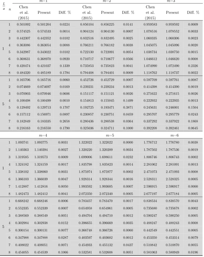
Tables 1 and 2 are regulated to compare the results of frequency analysis of a stepped shell with elas-tic ended supports using the proposed method and those reported in Qu et al. (2013) and Chen et al. (2015). Qu et al. (2013) have solved the issue of free and forced vibration analysis in a stepped shell with flexible ended supports using a numerical approach, modified variational principle and least-squares weighted residual method mixed by domain decomposition method (DDM). In a same man-ner, Chen et al. (2015) have utilized Flügge thin shell theory and the wave based method or WBM, and they have analyzed the same issue, adopted by Qu et al. (2013), under a point load excitation. Hence, by considering the presence of only one step at the shell geometry and neglecting the interior supports, i.e. (Km)i 0 in Eq. (19), as those in Qu et al. (2013) and Chen et al. (2015), a comparison
between the results of VWM and the results reported by Qu et al. (2013) and Chen et al.(2015) is performed. The results of this comparison are summarized in Table 1. The symbol of m in Table 1 denotes the axial mode number. As it can be seen in Table 1, there is a good agreement between the results of VWM and the results available in literature for the case of a stepped shell with flexible supports.
Table 2 shows the frequency analysis in free vibrations of a three stepped cylindrical shell with different axial lengths and SD-SD ended supports obtained by using VWM and the results obtained based on DDM by Qu et al. (2013) and WBM by Chen et al. (2015), respectively. By neglecting all flexible intermediate supports, namely (Km)i0 in Eq. (19), the present work is comparable with those reported by Qu et al. (2013) and Chen et al. (2013). Despite of differences in shell theory used by Qu et al. (2013), table 2 indicates a good proximity between all results obtained by the proposed method and those given in the literature.
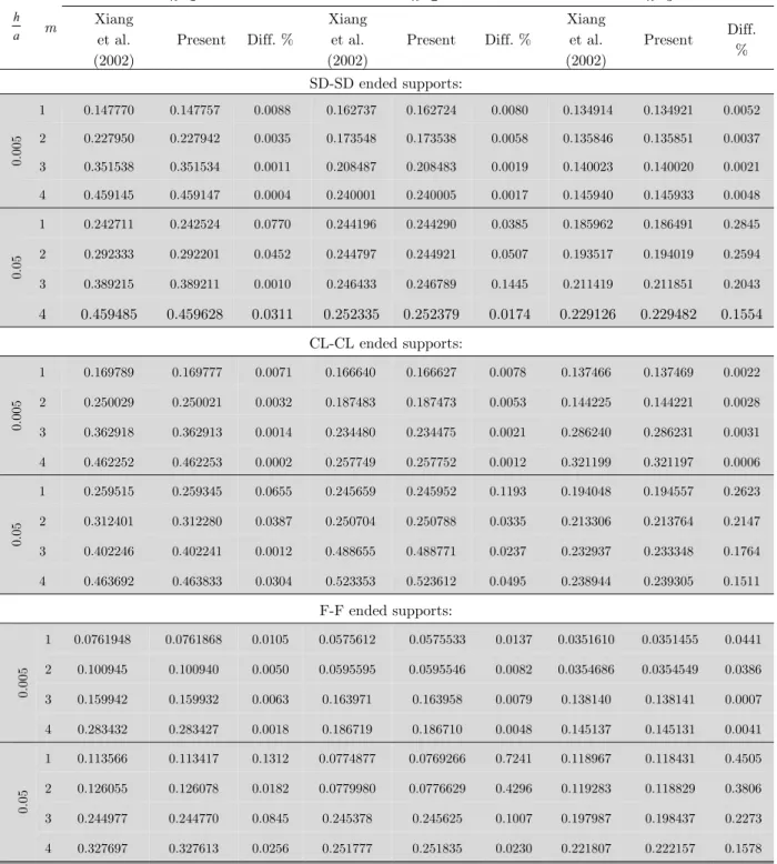
To examine the accuracy of the VWM in the presence of intermediate supports, the results of present method are compared with the results of Xiang et al. (2002). In the study of Xiang et al. (2002) presented an exact solution, a state-space technique (SST), to solve the problem of vibrations of a uniform circular cylindrical shell based on the Goldenveizer–Novozhilov shell theory by using different classic ended supports e.g. clamped (CL), SD, and free (F) supports and different numbers of intermediate rigid supports. In order to a possible comparison with the study of Xiang et al. (2002), the thickness of the shell in the present study should be considered as uniform. Hence, the interface matrices of ψand are required to be equal for each segment, i.e.
n ψ ψ
ψ1 2 ... and
1 2 ... n in Eq. (19). In fact, Eqs. (3) and (10) all are independent from the shell lengths in
a L
n
EI-EI EI-EII EII-EII
Chen et al. (2015)
Present Diff. %
Chen et al. (2015)
Present Diff. %
Qu et al. (2013)
Present Diff. %
1
1 0.596712 0.596719 0.0012 0.719461 0.719464 0.0004 0.377815 0.377816 0.0003
2 0.627766 0.627791 0.0040 0.467940 0.467963 0.0049 0.353129 0.353136 0.0020
3 0.467720 0.467728 0.0017 0.345921 0.345948 0.0078 0.330581 0.330589 0.0024
4 0.351454 0.351451 0.0009 0.285703 0.285739 0.0126 0.306288 0.306313 0.0082
5 0.275873 0.275865 0.0029 0.250598 0.250640 0.0168 0.282619 0.282650 0.0110
6 0.233051 0.233050 0.0004 0.230591 0.230627 0.0156 0.263490 0.263528 0.0144
7 0.216637 0.216641 0.0018 0.224561 0.224613 0.0232 0.252666 0.252711 0.0178
8 0.220472 0.220491 0.0086 0.231966 0.232013 0.0203 0.252516 0.252569 0.0210
5
1 0.179718 0.179721 0.0017 0.146093 0.146092 0.0007 0.145988 0.145996 0.0055
2 0.075177 0.075180 0.0040 0.085319 0.085330 0.0129 0.105754 0.105763 0.0085
3 0.042625 0.042623 0.0047 0.053657 0.053662 0.0093 0.070464 0.070476 0.0170
4 0.042376 0.042376 0.0000 0.049152 0.049158 0.0122 0.056729 0.056741 0.0212
5 0.054185 0.054366 0.3340 0.061281 0.061278 0.0049 0.062286 0.062295 0.0144
6 0.064989 0.064980 0.0138 0.072185 0.072352 0.2314 0.072185 0.072351 0.2300
7 0.078500 0.078543 0.0548 0.083644 0.083742 0.1650 0.083655 0.083744 0.1064
8 0.096959 0.096953 0.0062 0.100140 0.100140 0.0000 0.100140 0.100140 0.0000
10
1 0.059525 0.059532 0.0118 0.066987 0.066995 0.0119 0.080261 0.080261 0.0000
2 0.022017 0.022019 0.0091 0.029133 0.029135 0.0069 0.040165 0.040169 0.0100
3 0.020973 0.020969 0.0191 0.024247 0.024252 0.0206 0.027631 0.027644 0.0470
4 0.029436 0.029460 0.0815 0.033615 0.033674 0.1755 0.033626 0.033682 0.1663
5 0.038434 0.038432 0.0052 0.041343 0.041349 0.0145 0.041343 0.041350 0.0169
6 0.052156 0.052155 0.0019 0.053587 0.053596 0.0168 0.053587 0.053596 0.0168
7 0.069989 0.069990 0.0014 0.070660 0.070674 0.0198 0.070660 0.070674 0.0198
8 0.091235 0.091235 0.0000 0.091569 0.091576 0.0076 0.091569 0.091576 0.0076
Table 1: Natural frequency factor(Ω) and EI-EI, EII-EIIor EIII-EIII ended supports for a shell with one step (L
1/L=0.5
a L
n
m=1 m=2 m=3
Chen et al. (2015)
Present Diff. %
Chen et al. (2015)
Present Diff. %
Chen et al. (2015)
Present Diff. %
1
1 0.501092 0.501204 0.0224 0.856104 0.856225 0.0141 0.959583 0.959592 0.0009
2 0.574525 0.574533 0.0014 0.904124 0.904130 0.0007 1.078516 1.078552 0.0033
3 0.442307 0.442352 0.0102 0.832516 0.832495 0.0025 1.060335 1.060306 0.0023
4 0.363086 0.363054 0.0088 0.766211 0.766182 0.0038 1.045075 1.045096 0.0020
5 0.342987 0.343022 0.0102 0.722130 0.722091 0.0054 1.038734 1.038750 0.0015
6 0.368631 0.368970 0.0920 0.710717 0.710677 0.0566 1.046612 1.046620 0.0008
7 0.420474 0.421037 0.1339 0.735853 0.735823 0.0041 1.074990 1.072490 0.2326
8 0.484320 0.485189 0.1794 0.794408 0.794401 0.0009 1.118762 1.118737 0.0022
5
1 0.165706 0.165716 0.0060 0.452726 0.452729 0.0007 0.597709 0.597761 0.0087
2 0.074669 0.074697 0.0169 0.239231 0.239234 0.0013 0.414398 0.414390 0.0019
3 0.070903 0.070946 0.0606 0.151117 0.151121 0.0026 0.271622 0.271615 0.0026
4 0.100498 0.100499 0.0010 0.154813 0.155045 0.1499 0.222932 0.222935 0.0013
5 0.129492 0.129713 0.1707 0.192725 0.193471 0.3871 0.245631 0.246001 0.1504
6 0.157112 0.156971 0.0897 0.230857 0.230751 0.0459 0.295707 0.295779 0.0243
7 0.182849 0.183335 0.2658 0.280436 0.280538 0.0364 0.337292 0.337922 0.1868
8 0.216163 0.216550 0.1790 0.325036 0.324711 0.1000 0.392208 0.392461 0.0645
m=4 m=5 m=6
1
1 1.093741 1.093775 0.0031 1.322022 1.322022 0.0000 1.776712 1.776780 0.0038
2 1.140363 1.140394 0.0027 1.320220 1.320209 0.0034 1.787502 1.787536 0.0019
3 1.319585 1.319573 0.0009 1.699006 1.698611 0.0232 1.806746 1.806743 0.0002
4 1.324182 1.324159 0.0017 1.835798 1.835823 0.0014 2.281062 2.281091 0.0013
5 1.338102 1.338060 0.0031 1.875974 1.875977 0.0002 2.471073 2.471093 0.0008
6 1.366103 1.366039 0.0047 1.928314 1.928344 0.0016 2.528311 2.528325 0.0005
7 1.412887 1.412816 0.0050 1.993592 1.993605 0.0007 2.596915 2.596917 0.0000
8 1.482473 1.482412 0.0041 2.072350 2.072340 0.0005 2.677197 2.677184 0.0005
5
1 0.668242 0.668246 0.0006 0.783457 0.783470 0.0017 0.838534 0.838570 0.0043
2 0.552335 0.552339 0.0007 0.654958 0.654961 0.0005 0.735680 0.735678 0.0002
3 0.388569 0.388549 0.0051 0.494704 0.494710 0.0012 0.590247 0.590250 0.0005
4 0.302984 0.302938 0.0152 0.396655 0.396669 0.0035 0.488247 0.488243 0.0008
5 0.300154 0.300131 0.0077 0.366748 0.366726 0.0060 0.442549 0.442551 0.0005
6 0.347988 0.347888 0.0287 0.403597 0.403602 0.0012 0.453350 0.453314 0.0079
7 0.408022 0.408051 0.0071 0.454933 0.455132 0.0437 0.510842 0.510870 0.0055
8 0.454055 0.454539 0.1066 0.532581 0.532608 0.0051 0.581063 0.580949 0.0196
Table 2: Comparison of frequency factors for a three-stepped cylindrical shell with SD–SD ended supports
a h
m
n=1 n=2 n=3
Xiang et al. (2002)
Present Diff.%
Xiang et al. (2002)
Present Diff.% Xiang
et al. (2002)
Present Diff.%
SD-SD ended supports:
0.005
1 0.130008 0.129997 0.0085 0.132434 0.132425 0.0068 0.0817846 0.0817907 0.0075
2 0.216851 0.216845 0.0028 0.139345 0.139341 0.0029 0.090776 0.090780 0.0044
3 0.327090 0.327091 0.0003 0.153293 0.153296 0.0020 0.106105 0.106104 0.0009
4 0.474651 0.474648 0.0006 0.289228 0.289220 0.0028 0.217507 0.217501 0.0028
0.05
1 0.204520 0.204384 0.0665 0.160475 0.160759 0.1770 0.144682 0.145056 0.2585
2 0.259187 0.259133 0.0208 0.169728 0.169955 0.1337 0.153609 0.153971 0.2357
3 0.327216 0.327314 0.0299 0.188408 0.188529 0.0642 0.172214 0.172537 0.1876
4 0.511623 0.511620 0.0006 0.375113 0.375292 0.0477 0.298856 0.299616 0.2543
CL-CL ended supports:
0.005
1 0.154336 0.154327 0.0058 0.136457 0.136449 0.0059 0.0933758 0.0933801 0.0046
2 0.241012 0.241016 0.0017 0.167033 0.167028 0.0030 0.115563 0.115565 0.0017
3 0.338453 0.338454 0.0003 0.179008 0.179009 0.0006 0.119640 0.119640 0.0000
4 0.476570 0.476568 0.0004 0.295883 0.295877 0.0020 0.221095 0.221091 0.0018
0.05
1 0.223084 0.222963 0.0427 0.173642 0.173884 0.1394 0.153883 0.154251 0.2391
2 0.283979 0.283930 0.0173 0.201442 0.201634 0.0953 0.173379 0.173727 0.2007
3 0.340111 0.340211 0.0294 0.207148 0.207303 0.0748 0.183228 0.183538 0.1692
4 0.512793 0.512791 0.0004 0.378227 0.378412 0.0489 0.306910 0.307603 0.2258
F-F ended supports:
0.005
1 0.0497717 0.0497667 0.0100 0.0364021 0.0363968 0.0146 0.0209389 0.0209242 0.0702
2 0.0803789 0.0803745 0.0055 0.0388606 0.0388548 0.0149 0.0247300 0.0247157 0.0578
3 0.149512 0.149505 0.0047 0.134440 0.134432 0.0060 0.0973975 0.0973995 0.0021
4 0.287551 0.287546 0.0017 0.185029 0.185020 0.0049 0.126344 0.126340 0.0032
0.05
1 0.0732860 0.0732042 0.1116 0.0551522 0.0547287 0.7679 0.113302 0.112977 0.2868
2 0.0962236 0.0962061 0.0182 0.0594661 0.0590527 0.6952 0.114218 0.113873 0.3021
3 0.211456 0.211316 0.0662 0.180577 0.180752 0.0969 0.158907 0.159146 0.1504
4 0.331141 0.331067 0.0223 0.230678 0.230608 0.0303 0.189382 0.189292 0.0475
Table 3: Comparison of frequency factor, Ω, for a shell with two intermediate ring supports and different
thicknesses and ended supports conditions.
presence of different numbers of intermediate RS. Again, a good proximity can be seen in the ob-tained results by the two methods applied.
a h
m
n=1 n=2 n=3
Xiang et al. (2002)
Present Diff. %
Xiang et al. (2002)
Present Diff. % Xiang
et al. (2002)
Present Diff. % SD-SD ended supports:
0.005
1 0.147770 0.147757 0.0088 0.162737 0.162724 0.0080 0.134914 0.134921 0.0052
2 0.227950 0.227942 0.0035 0.173548 0.173538 0.0058 0.135846 0.135851 0.0037
3 0.351538 0.351534 0.0011 0.208487 0.208483 0.0019 0.140023 0.140020 0.0021
4 0.459145 0.459147 0.0004 0.240001 0.240005 0.0017 0.145940 0.145933 0.0048
0.05
1 0.242711 0.242524 0.0770 0.244196 0.244290 0.0385 0.185962 0.186491 0.2845
2 0.292333 0.292201 0.0452 0.244797 0.244921 0.0507 0.193517 0.194019 0.2594
3 0.389215 0.389211 0.0010 0.246433 0.246789 0.1445 0.211419 0.211851 0.2043
4 0.459485 0.459628 0.0311 0.252335 0.252379 0.0174 0.229126 0.229482 0.1554 CL-CL ended supports:
0.005
1 0.169789 0.169777 0.0071 0.166640 0.166627 0.0078 0.137466 0.137469 0.0022
2 0.250029 0.250021 0.0032 0.187483 0.187473 0.0053 0.144225 0.144221 0.0028
3 0.362918 0.362913 0.0014 0.234480 0.234475 0.0021 0.286240 0.286231 0.0031
4 0.462252 0.462253 0.0002 0.257749 0.257752 0.0012 0.321199 0.321197 0.0006
0.05
1 0.259515 0.259345 0.0655 0.245659 0.245952 0.1193 0.194048 0.194557 0.2623
2 0.312401 0.312280 0.0387 0.250704 0.250788 0.0335 0.213306 0.213764 0.2147
3 0.402246 0.402241 0.0012 0.488655 0.488771 0.0237 0.232937 0.233348 0.1764
4 0.463692 0.463833 0.0304 0.523353 0.523612 0.0495 0.238944 0.239305 0.1511
F-F ended supports:
0.005
1 0.0761948 0.0761868 0.0105 0.0575612 0.0575533 0.0137 0.0351610 0.0351455 0.0441
2 0.100945 0.100940 0.0050 0.0595595 0.0595546 0.0082 0.0354686 0.0354549 0.0386
3 0.159942 0.159932 0.0063 0.163971 0.163958 0.0079 0.138140 0.138141 0.0007
4 0.283432 0.283427 0.0018 0.186719 0.186710 0.0048 0.145137 0.145131 0.0041
0.05
1 0.113566 0.113417 0.1312 0.0774877 0.0769266 0.7241 0.118967 0.118431 0.4505
2 0.126055 0.126078 0.0182 0.0779980 0.0776629 0.4296 0.119283 0.118829 0.3806
3 0.244977 0.244770 0.0845 0.245378 0.245625 0.1007 0.197987 0.198437 0.2273
4 0.327697 0.327613 0.0256 0.251777 0.251835 0.0230 0.221807 0.222157 0.1578
Table 4: Comparison of frequency factor, Ω, for a shell with three intermediate ring supports and
a L
a h
SD-SD CL-CL F-F Xiang et
al. (2002) Present
Xiang et
al. (2002) Present
Xiang et
al. (2002) Present Two numbers of RS at L1/a= L2/a=1/3
5 0.005 0.0973341
(n=7) 0.0973576
0.106083
(n=7) 0.106105
0.0437255
(n=5) 0.0436924
5 0.05 0.306629
(n=4) 0.307444
0.313202
(n=3) 0.313855
0.115637
(n=1) 0.115475
10 0.005 0.04757610
(n=5) 0.04758732
0.0529403
(n=5) 0.0529510
0.0209389
(n=3) 0.0209224
10 0.05 0.14468164
(n=3) 0.14505607
0.153883
(n=3) 0.154251
0.0551522
(n=2) 0.0551473
Three numbers of RS at L1/a= L2/a= L3/a =1/4
1 0.005 0.130529
(n=8) 0.130560
0.136550
(n=8) 0.136581
0.0602356
(n=5) 0.0601946
1 0.05 0.393468
(n=1) 0.393128
0.405710
(n=4) 0.406755
0.176555
(n=1) 0.176349
5 0.005 0.0652931
(n=6) 0.0653081
0.0686462
(n=6) 0.0686610
0.0293818
(n=4) 0.0293592
5 0.05 0.185962
(n=3) 0.186491
0.194048
(n=3) 0.194557
0.113566
(n=1) 0.113417
Table 5: Comparison of fundamental frequency factor,
f
, in the presence of various numbers of intermediate RS.
Figures 6 show the effect of the wave barriers location on the natural frequencies of circular cy-lindrical shells. Here, the examined barriers are of type of shell step and intermediate radial supports (RS). In order to make a fair comparison, all conditions are considered the same as those given in Chen et al. (2015). Hence, the geometrical and mechanical considerations in the presence and the absence of the intermediate support are as follows: the thickness ratio h1/a=0.01, the step thickness ratio h1/h2=0.25, 0.5, 2, and 4, the length to radius ratio L/a=5, and 10 and finally step location (and intermediate support location) is at L1/L=0.5. Figures 6 show that the obtained results in the absence of the intermediate support have good agreement with those reported in the literature (Chen et al. (2015)).
Great impact of the existence of interior support on increasing of both beam mode- and funda-mental-frequency factors is clearly visible in the all cases considered for Figures 6. It is a very logical phenomena where happened due to the increase of the whole system rigidity, affected by the applied interior support. Hence, depending on the thickness ratio h2/h1, the greatest variation of all frequen-cies approximately, occurs for the intermediate type of RS, applied in an interval of 0.4<L1/L<0.6. As it can be seen in these figures, the maximum fundamental frequency factor for all of the shell length ratios, i.e. L/a=5 and 10, in the presence of intermediate RS, happened in thickness ratio of
h2/h1=0.25 and in the position ratio of L1/L=0.4. However, in the case of maximum beam mode fre-quency factor, depending on the shell length ratio, it happens in thickness ratio of h2/h1=0.25 for
a) b)
c) d)
Figure 6: Beam mode- (a,c) and fundamental-frequency parameters (b,d) versus the location of the wave barrier,
L1/L, for a SD–SD shell with (---) and without (____) intermediate support —□— h1/h2=2, —○—h1/h2=0.5, —
Δ— h1/h2=4, and—◊— h1/h2=0.25 including geometrical characteristics of: (a,b) L/a=5 and (c,d) L/a=10.
6.1.2 Mode Shapes
Using Eq. (26) or (34), it is possible to obtain all mode shapes of the cylindrical shell. In this section, radial mode shapes for beam modes, i.e. n=m=1, in the axial directions of a shell with different num-bers of intermediate RS and SD-SD ended supports are plotted in Figures 7 to 9 (By these considera-tions we are able to tracing satisfaction of the support condiconsidera-tions and continuity, simultaneously). Two cases for examination their mode shapes are considered here. In the first case a uniform shell and in the next case a stepped shell with different numbers of intermediate ring supports are consid-ered here.
In the case of a uniform shell, the effects of shell thickness on mode shapes corresponding with beam mode frequencies are depicted in Figures 7 for two shell lengths, i.e. L/a=10 and 5, respective-ly. In this figure, the normalized radial displacement are plotted for h/a=0.01, 0.05 and 0.1 in the presence of three numbers of intermediate RS. Due to the geometry and support condition chosen for the issue, symmetrical mode shapes are expected. As can be seen in these figures, the slope of the
0 0.2 0.4 0.6 0.8 1 0.14
0.16 0.18 0.2 0.22 0.24
Wave Barrier Location(L1/L)
Frequency Parameter (
Ω
)
0 0.2 0.4 0.6 0.8 1 0.02
0.04 0.06 0.08 0.1 0.12 0.14
Wave Barrier Location(L1/L)
Fundamental Frequency (
Ωf
)
0 0.2 0.4 0.6 0.8 1 0.04
0.06 0.08 0.1 0.12 0.14
Wave Barrier Location(L1/L)
Frequency Parameter (
Ω
)
0 0.2 0.4 0.6 0.8 1 0.01
0.02 0.03 0.04 0.05 0.06 0.07
Wave Barrier LocationL1/L
Fundamental Frequency (
Ωf
radial displacement fields, i.e. dUr/dx, at all support positions decreases in the thicker and shorter
cylindrical shells. Also, the shorter cylinders have higher sensitivity to the shell thickness.
a) b)
Figure 7: Mode shapes of a homogeneous SD-SD shell with three intermediate ring supports for m=n=1
(beam mode) and in different conditions as: h/a=0.01, 0.05, 0.1 a) L/a=10 b) L/a=5.
The mode shapes of the shell with different numbers of intermediate RS corresponding with beam mode frequencies are plotted in Figures 8 for two shell lengths, i.e. L/a=10 and 5, respectively. Hence, three cases are considered in these figures. Case 1-1: one intermediate RS at L1/L =0.25, Case 2-1: two numbers of intermediate RS at L1/L = L2/L =0.25, and Case 3-1: three numbers of inter-mediate RS at L1/L = L2/L = L3/L =0.25. In these figures, satisfying of continuity and all the sup-port conditions applied to such unsymmetrical conditions can be seen obviously in the all given re-sults.
In Figures 9a to 9f, radial mode shapes are depicted in the axial direction of a stepped shell with different combinations of intermediate ring supports. Hence, three cases of shell thickness and steppes are considered as: Case 1-2: uniform Shell, Case 2-2: three steppes in the shell; L1/L= L2/L =L3/L=0.25 and h1/a=0.01, h2/h1=2, h3/h2=3 and h4/h3=4 and finally Case 3-2: with same condition by case 2-2 except thicknesses of h2/h1=3, h3/h2=5 and h4/h3=7. In Figures 9a, 9c and 9e total shell length is L/a=5 and shell length that considered in Figures 9b, 9d and 9f is L/a=5. Number of the interior supports used in these figures is respectively as one interior support at L1/L=0.5 in Figures 9a and 9b, two interior ring supports at L1/L=L3/L=0.25 in Figures 9c and 9d and three interior supports at L1/L= L2/L= L3/L=0.25 in Figures 9e and 9f. These figures indicate that continuity and support conditions of the issue are completely satisfied by the proposed method, simultaneously. However by changing the shell thickness from case 1-2 to case 3-2, radial deformations in normalized modes are graded and mostly tended to the thinner sides of the shell.
6.2 Forced Vibration
In this section a stepped circular cylindrical shell with SD-SD ended supports and three intermediate supports of different types is considered. Other considerations are: Length ratio, L/a=5, thickness ratios h1/a=0.01 and h2/h1=2, h3/h2=2, h4/h3=2. In all of the following figures, the amplitude of the point load excitation is considered 100 N. The point loading are applied on the shell at 0
0 and
0 2 4 6 8 10
0 0.2 0.4 0.6 0.8 1 1.2
x (m)
Normalized
Ur
h/a=0.01 h/a=0.05 h/a=0.1
0 1 2 3 4 5
0 0.2 0.4 0.6 0.8 1 1.2
x (m)
Normalized
Ur
x/L=1/8 imposed at thinnest segments of the shell. In all graphs of frequency responses, frequency ranges are considered from 100 to 500 Hz and their steps are 2 Hz.
a) b)
Figure 8: Mode shapes corresponding with beam mode of the shell with h/a=0.05 and SD-SD ended supports
in three cases of numbers of applied intermediate RS and two shell lengths of a) L/a=10 b) L/a=5.
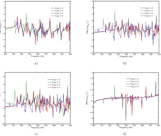
6.2.1 Verification of VWM Results
To achieve accurate results with low calculation time, minimum numbers of truncation of circumfer-ential mode number, n, which was described in Sec. 6, is required to be determined. Figures 10 de-picts the radial and circumferential displacement responses due to excitation of a point load ( 0 100N
r
f ) exactly at the middle of the first segments of the shell (x1=L1/2 in Figure 5) in the ra-dial direction. The results of these figures are plotted for some different truncation of n. In these fig-ures, a good convergent results for all truncations, i.e. n=20, 30 and 40, is clearly visible. However, the differences between results of n=30 and 40 are negligible, and hence, n=30 is chosen for evaluat-ing and plottevaluat-ing the Frequency Response Functions (FRF). Usevaluat-ing VWM and with the non-optimized self-writing code, the mean elapsed time for calculation when n=30 was about 12.09 seconds.
Due to lack of proper comparison results in the literature to evaluate the required VWM solution time and its numerical performance, we have utilized the finite element method provided by ANSYS for validation and evalution of the results. The forced vibration analysis given by VWM for classical ended and intermediate supports, i.e. SD and RS is considered. Then, utilizing ANSYS, an excited shell with a point load at the middle of the first segment as the thinnest segment of the stepped shell is modeled using the four node elements of shell 63.
Among several compositions of mapped meshing, three different meshing styles are chosen for evaluation of FEM convergence. These cases are: Case 1-3: 60 100, Case 2-3:80 120 and Case 3-3: 100 140 nodes in the and x directions, respectively. The results of ANSYS for different grid sizes of cases 1-3 to 3-3 are plotted in Figures 10c and 10d. As it can be seen from Figures 10c and 10d, cases 2-3 and 3-3 are convergent and approximately can cover all possible peaks correspond with all the natural frequencies. In an overall comparison between the results of VWM and the results of ANSYS as a FEM, the results of both methods are in good agreement in the case 2-3 for both of the radial and axial displacement responses. These comparisons between VWM and FEM are made in the
Fig-0 1 2 3 4 5 6 7 8 9 10 0
0.2 0.4 0.6 0.8 1
x (m)
Normalized
U
r
Case 1−1 Case 2−1 Case 3−1
0 0.5 1 1.5 2 2.5 3 3.5 4 4.5 5 0
0.2 0.4 0.6 0.8 1 1.2
x (m)
Normalized
U
r
urfes 10e and 10f. The computational time for calculations of case 2-3 was about 32 minutes using two CPU cores where is approximately 159 times greater than those given by VWM, utilizing only one CPU core.
a) b)
c) d)
e) f)
Figure 9: Mode shapes of a shell corresponding with beam mode (n=m=1) and shell lengths of a,c,e)
L/a=10 and b,d,f) L/a=5: a,b) One (at L1/L=0.5) c,d) two (at L1/L= L3/L=0.25) and e,f) three
(at L1/L= L2/L= L3/L=0.25) intermediate supports in three different cases of stepped shells. 0 1 2 3 4 5 6 7 8 9 10
−0.2 0 0.2 0.4 0.6 0.8 1
x (m)
Normalized
U’
r
Case 1−2 Case 2−2 Case 3−2
0 0.5 1 1.5 2 2.5 3 3.5 4 4.5 5 −0.2
0 0.2 0.4 0.6 0.8 1
x (m)
Normalized
U’
r
Case 1−2 Case 2−2 Case 3−2
0 1 2 3 4 5 6 7 8 9 10 −0.2
0 0.2 0.4 0.6 0.8 1
x (m)
Normalized
U’
r
Case 1−2 Case 2−2 Case 3−2
0 0.5 1 1.5 2 2.5 3 3.5 4 4.5 5 −0.2
0 0.2 0.4 0.6 0.8 1
x (m)
Normalized
U’
r
Case 1−2 Case 2−2 Case 3−2
0 1 2 3 4 5 6 7 8 9 10 −0.2
0 0.2 0.4 0.6 0.8 1
x (m)
Normalized
U’
r
Case 1−2 Case 2−2 Case 3−2
0 0.5 1 1.5 2 2.5 3 3.5 4 4.5 5 −0.2
0 0.2 0.4 0.6 0.8 1
x (m)
Normalized
U’
r