J. Aerosp. Technol. Manag. vol.4 número3

LIST OF SYMBOLS

a_ijk Membrane compliance term for composite adherent  k, k =1,2,3

b_ijk Coupling compliance term for composite adherent  k, k =1,2,3

d_ijk Bending­torsion  compliance  term  for  composite  adherent k, k =1,2,3

E₁ <RXQJPRGXOXVLQ¿EHUGLUHFWLRQ

E₂ <RXQJPRGXOXVLQWUDQVYHUVHGLUHFWLRQRIWKH¿EHU G₁₂ Shear modulus in ply plane

E_a Adhesive young modulus G_a Adhesive shear modulus

u₀i Middle plane adherent displacement in x direction  for adherent i, i =1,2,3

v₀i Middle plane adherent displacement in y direction  for adherent i, i =1,2,3

wi Adherent  displacement  in z  direction  for  adherent i,  i =1,2,3

N_xi _{Normal force in x direction for adherent i, i =1,2,3} N_yi _{Normal force in y direction for adherent i, i =1,2,3} Q_xi 6KHDUIRUFHLQWKH[IDFHRILQ¿QLWHVLPDOHOHPHQWIRU

adherent i, i =1,2,3

Q_yi 6KHDUIRUFHLQWKH\IDFHRILQ¿QLWHVLPDOHOHPHQWIRU adherent i, i =1,2,3

M_xxi _{Moment around x axis for adherent i, i =1,2,3} M_yyi _{Moment around y axis for adherent i, i =1,2,3} M_xyi Moment around y axis in the xIDFHRILQ¿QLWHVLPDO

element for adherent i, i =1,2,3

M_yxi Moment around x axis in the yIDFHRILQ¿QLWHVLPDO element for adherent i, i =1,2,3

t_i Thickness of the adherent i, i =1,2,3 t_ai Thickness of the adhesive layer i, i =1,2 ıazj

Normal  stress  in  adhesive  layer  in z  direction  for  adhesive j, j =1,2

IJaxj

Shear  stress  in  adhesive  layer  in xz  plane  for  adhesive j, j =1,2

IJayj

Shear  stress  in  adhesive  layer  in yz  plane  for  adhesive j, j =1,2

ȣ 3RLVVRQVFRHI¿FLHQW

INTRODUCTION

  In  the  last  years,  the  usage  of  composite  materials  as  a  primary  structural  element  has  increased.  Some  new  aircraft  designs, such as Airbus A380 and Boeing 787, use composite  materials even for primary structural elements, such as wing  spars and fuselage skins, achieving lighter structures without  reducing of airworthiness. One way to assemble those parts is  to apply a bonded joint, which possesses some advantages, for 

Bonded Joints Design Aided by Computational Tool

Marcelo L. Ribeiro*, Volnei Tita

Escola de Engenharia de São Carlos/Universidade de São Paulo – São Carlos/SP­ Brazil

Abstract: In order to aid the design of bonded joints, a computational tool named System of Analysis for Joints (SAJ) was  developed. The software can analyze single and double lap bonded joint with composite­composite or metal­composite mate­ rials as adherent parts. Thus, SAJ can calculate the stress distribution, loads and displacements. Their results were compared  WR¿QLWHHOHPHQWVRIWZDUH$%$486TMDQGWRVSHFL¿FFRPSRVLWHDQDO\VLVVRIWZDUH(6$&RPSTM_{). After that, a study about the}  LQÀXHQFHRIMRLQWGHVLJQSDUDPHWHUVRQWKHPHFKDQLFDOEHKDYLRURIWKHERQGHGMRLQWZDVFDUULHGRXW,QUHJDUGVWRSDUDPHWULF study, SAJ leads to some conclusions, which can be used as a guide during the product design process. Therefore, aided by  the computational tool, it is possible to perform a conceptual and preliminary design of bonded joints with more accuracy  DQGYDU\LQJPDQ\SDUDPHWHUVPDWHULDOV¿EHURULHQWDWLRQDQGVWDFNLQJVHTXHQFHRIWKHODPLQDWHWKLFNQHVVRYHUODSOHQJWK

Keywords:%RQGHGMRLQWV'HVLJQSDUDPHWHUV&RPSRVLWHMRLQWV&RPSXWDWLRQDOWRRO$GKHVLYHV6WUHVVDQDO\VLV

Received: 15/05/12  Accepted: 02/07/12 *author for correspondence: malribei@usp.br

example: better fatigue endurance; joining dissimilar materials;  better insulation; smooth surface and lower weight. However,  there are also negative aspects, for example: no possibility to  disassemble the joints; peeling stress should be minimized and  the preparation of the surfaces for bonding must be done care­ IXOO\0RUWHQVHQ%HVLGHVLWLVYHU\GLI¿FXOWWRSUHGLFWWKH stress distribution in bonded joints and many design parameters  LQÀXHQFHWKHPHFKDQLFDOEHKDYLRURIWKLVW\SHRIMRLQW

  Regarding this scenario, many researchers have conducted  studies about bonded joints, trying to predict their mechani­ FDO EHKDYLRU E\ ¿QLWH HOHPHQW PRGHOV DQDO\WLFDO PRGHOV experimental tests or hybrid approaches, combining theoreti­ FDODQGH[SHULPHQWDODQDO\VHV7KH¿UVWDQDO\VHVIRUERQGHG joints  were  carried  out  by  Volkersen  in  1938  (Mortensen,  1998). Volkersen modeled the adhesive layer as shear spring  GLVWULEXWHGRYHUWKHGRXEOHODSMRLQWGLVUHJDUGLQJWKHÀH[­ ural effects (Mortensen, 1998). The results obtained by the  researcher showed that the load transfer at the adhesive was  not  uniform.  Goland  and  Reissner  (1944)  improved  Volk­ ersen’s  model  by  considering  the  adherent  like  beams  and  the adhesive like springs in tension and shear loading. That  model could analyze the distribution of the transversal load­ ing induced by the secondary moment, which occurs in single  lap joints. Hart­Smith (1970; 1973), based on the last models,  LQWURGXFHGWKHLQÀXHQFHRIWKHWKHUPDOH[SDQVLRQEHWZHHQWKH materials. Hart­Smith simulated the adhesive response, using  an elastic­plastic material model. It is important to mention  WKDW+DUW6PLWKLQYHVWLJDWHGWKHLQÀXHQFHRI the main design parameters in the structural performance of  the joint too. However, some of those models assumed that  the laminates were isotropic or symmetric (only with tension  DQGÀH[XUDOVWLIIQHVVGLVUHJDUGLQJWKHOD\HUVDQGFRQVLGHU­ ing apparent properties for the laminates. In 1975, Yuceoglu  and Updike improved Hart­Smith’s model by considering the  transversal shear effects in the adherent. They showed that  LIWKHDGKHUHQWVKDYHVWURQJDQLVRWURS\DQGKLJKHUÀH[LELO­ ity in shear loading, the normal strains can affect the stress  distribution in the adhesive. Thomsen (1992) showed that an  increase in the overlap length reduces the stress level in the  adhesive layer. The researcher concluded that the application  of adhesive layer with lower elastic shear and tensile moduli  GHFUHDVHVWKHDGKHVLYHVWUHVV7KRPVHQYHUL¿HGWKDWLW is better to use identical or nearly identical adherents in bond­ ed joints, i.e., adherents with similar stiffness. Frostig et  al_.  (1998) proposed an approach using high­order theory. In their  analysis, the adhesive was modeled as an elastic continuum  media (2D and 3D). So, the adhesive could transfer normal 

stresses, in­plane and transversal shear stresses. These results  showed that there was a great variation of the normal stress in  the adhesive close to the edges.

with warping effects. Agnieszka (2009) showed a numerical  method,  regarding  the  sensitivity  to  hydrostatic  stress  for  prediction of the delamination initiation. This method allows  simulating the failure in the joint (at the overlap region) and  in the adherent. Silva et al_{. (2009a; 2009b) showed an excel­} lent bibliographic review about models for bonded joints and  performed a comparison between the most important models,  showing the advantages and limitations for each one. More  UHFHQWO\ ;LDRFRQJ VKRZHG D UHYLHZ DERXW ¿QLWH element method applied to simulate bonded joints.

  In many studies commented earlier, the researches proved  WKDWGLIIHUHQWGHVLJQSDUDPHWHUVFDQLQÀXHQFHWKHPHFKDQLFDO behavior of bonded joints due to the interaction phenomena  (for  example:  mechanical,  physical  and  chemical  interac­ tions) between parts (adherents) and adhesives. Besides, the  W\SHRIWKH¿EHUDQGWKHPDWUL[RIWKHFRPSRVLWHDVZHOODV the stacking sequence of the laminate can change the struc­ tural performance of the bonded joints. Therefore, it can be  concluded that the design and analysis of bonded joints is very  complex problem, which there is not still a closed solution.  Thus, new proposals to solve this problem are required.   In  order  to  aid  the  design  of  bonded  joints,  a  computa­ tional tool named System of Analysis for Joints (SAJ) was  developed, which is capable of analyzing not only single lap  joint, but also double lap joint. These joints could be made  of composite­composite materials or dissimilar materials, i.e.,  metal­composite. For both types of joints, SAJ can calculate  the stress and strain distributions, loads and displacements. In  order to evaluate the limitations and advantages of the SAJ,  some analyses were performed, using case studies. Moreover  WKH 6$- UHVXOWV ZHUH FRPSDUHG WR ¿QLWH HOHPHQW VRIWZDUH (ABAQUSTM DQG WR VSHFL¿F FRPSRVLWH DQDO\VLV VRIWZDUH (ESACompTM$IWHU WKDW D VWXG\ DERXW WKH LQÀXHQFH RI bonded joint design parameters on its mechanical behavior  was carried out (overlap length; type of joint; adhesive elastic  modulus and adhesive layer thickness).

THE COMPUTATIONAL TOOL – SAJ

  The computational tool was developed to calculate the joint  loads,  displacements  and  adhesive/adherents  stresses  with  non­linear effects (Ribeiro et  al._{, 2010). This computational}  tool named SAJ was programmed in MatlabTM _{language and}  can analyze single and double lap bonded joints. In fact, SAJ  can predict the mechanical behavior of composite­composite  and  metal­composite  bonded  joints.  Regarding  composite 

adherents, the computational tool can calculate the stress and  strain distributions in each layer of the laminate.

  To predict the mechanical behavior of bonded joints, SAJ  UHDGVDQLQSXW¿OHZLWKGDWDRIDGKHUHQWVDGKHVLYHDQGMRLQW FKDUDFWHULVWLFV7KLV¿OHFRQWDLQVLQIRUPDWLRQVXFKDVOD\XSDQG layer thickness in case of composite adherents, mechanical prop­ erties for adherents and adhesives, joint dimensions of adhesive  and adherents, as well as loads and boundary conditions. Using  the input data, SAJ builds a set of differential equations, which is  solved by MatlabTM_{. After that, SAJ shows forces, displacements}  and adhesive stresses by graphics and tabular format.

Mathematical formulation

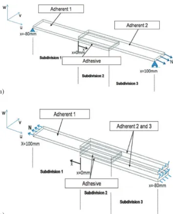
  A set of differential equations of the multi­domain bound­ ary value problem is implemented in SAJ. In order to obtain  this set of differential equations, the problem domain (bonded  joint) is partitioned in three regions: one part for adherents  only, other part for the bonded region (overlap region) and  the last part, again, only for adherents. Figure 1 shows these  subdivisions,  coordinate  system,  as  well  as  an  example  of  boundary conditions and loads for single lap joint (Fig. 1a)  and double lap joint (Fig. 1b).

(a)

(b)

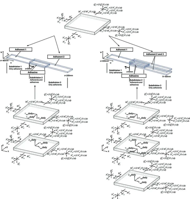
  For each region, free body diagrams of equilibrium in an  LQ¿QLWHVLPDOYROXPHHOHPHQWFDQEHREWDLQHGDVVKRZQLQ)LJ Thus, the set of differential equilibrium equations for single and  double lap joints can be written. Based on these equations and  applying the hypothesis that all derivatives in y direction are  equal to zero (cylindrical bending hypothesis), as well as consid­ ering plane stress state and Kirchhoff’s kinematic relations, it 

is possible to obtain the set of differential equations shown by  Fig. 2 For composite adherents, some terms of the equations  are calculated using the CLT and the symbols a_ij, b_ij and d_ij at  Fig. 2 correspond to components of laminate compliance matrix.  The membrane, coupling and bending­torsion compliances are  represented by a_ij, b_ij and d_ij, respectively. Also, at the Fig. 3, the  sub index comma with “x” means partial derivate in “x”.

Read input data Calculus of Stiffness matrix Calculus of Compliance matrix Solve the boundary value problem (bvp4c) Results )LJXUH*HQHUDOÀRZFKDUWRI6\VWHPRI$QDO\VLVIRU-RLQWV   Using the free­body diagrams (Fig. 2) and CLT, the set of  equations for the subdivisions out of overlap region (single  or double lap joint) is presented in Eq. 1. The upper letter i  (i _{= 1, 2, 3) indicates the adherent.}

  (1) 0 0 0 0 0 0 0

u a N a N b M

w k

k b N b N d M

v a N a N b M

N N M Q 0 , , , , , , , x i i xx i i xy i i xx i xx i x i x i i xx i i xy i i xx i x i i xx i i xy i i xx i xx x i xy x i xx x i x x i

0 11 13 11

11 13 11

0 21 23 21

‐ ‐ ‐ = + = ‐ ‐ ‐ = ‐ ‐ ‐ = = = = =   Regarding the double lap joint, the same procedure described  before (free­body diagrams and CLT) is used to obtain the set  of differential equations for double lap joint adherent 1 (Fig. 2).  Equation 2 shows the set of differential equations for this region.   (2) 0 0 0 0 0 0 0

u a N a N b M

w k

k b N b N d M

v a N a N b M

N

N

M Q t t t t

Q 2 2 0 , , , , 1 , , 1 1 2

, 1 2

x xx xy xx

xx x

x xx xy xx

x xx xy xx

xx x ax ax xy x ay ay

xx x x ax a

ax a

x x az az

0 1 11 1 1 13 1 1 11 1 1 1 1 1 11 1 1 13 1 1 11 1 1 0 1 21 1 1 23 1 1 21 1 1 1 2 1 1 2 1 1 1 1 2 1 x x x x x x v v ‐ ‐ ‐ = + = ‐ ‐ ‐ = ‐ ‐ ‐ = + ‐ = + ‐ = ‐ + + ‐ + = ‐ + =

^ h ^ h

  For the other regions in the overlap area (double and single lap  joint), the resulting set of differential equations is presented in Eq. 3.  In this case, the upper letter i (i _{= 1, 2) indicates the adherent for single} 

lap joint or i ₍i _{= 2, 3) indicates the adherent for double lap joint.}

  (3)

u a N a N b M

w k

k b N b N d M

v a N a N b M

N

N

M Q t t

Q 0 0 0 0 0 0 2 0 0 , , , , , , 1 , x i i xx i i xy i i xx i xx i x i x i i xx i i xy i i xx i x i i xx i i xy i i xx i xx x i ax xy x i ay xx x i x i ax a x x i az

0 11 13 11

11 13 11

0 21 23 21

x x x v ‐ ‐ ‐ = + = ‐ ‐ ‐ = ‐ ‐ ‐ = + = + = ‐ + + = ‐ = ^ h   It is important to mention that the adhesive is simulated  as springs under tension or compression combined to shear  stresses as shown by the following equations: ( ) ( ) t G

u t x k u t x k

2 2

1

ax a

a i i

x

i i i

x i

0 0

1 1

$ $

x = ‐ ‐ + ‐

+ +

c m   (4)

t G

v v

ay a

a i i

0 0

1

x = ^ ‐ +h   (5)

t E

w w 1

az a

a i i

v = ^ ‐ +h   ₍₆₎

where t

i is the thickness of the i adherent (i = 1, 2, 3), ta is the 

adhesive thickness, țx is the rotation at the x _axis, u 0 is the  middle plane displacement in x _{direction and} v

0 is the middle  plane displacement in y direction.

  Regarding  the  boundary  conditions,  in  general  they  are  provided as forces, moments or displacements in the edges of  the problem domain which will be described in more detail in  the following sections.

  Finally, the differential equations for each subdivision are  solved  using  MatlabTM_{,  which  can  deal  with  multi­domain}  boundary value problem, also each subdivision are divided in  n parts (mesh). It is important to mention that the ESACompTM  has basically the same formulation used in SAJ, but the solv­ ing process is different. Numerical analyses procedure   The numerical analysis starts after SAJ reads input data from  D¿OHZKLFKSUHVFULEHWKHMRLQWW\SHVLQJOHRUGRXEOHDGKHUHQWV and adhesives mechanical properties, ply thickness and orienta­ tion (in case of composite materials), adhesive thickness and the  dimensions, as well as loads and boundary conditions. Based  on these data, SAJ calculates the stiffness and the compliance  matrix. For composite parts (adherents), the CLT is applied.   Knowing the joint type, the boundary conditions and the  compliance matrix calculated in a previous step, SAJ builds  the set of differential equations presented earlier. This set of  equations comprises on a boundary value problem, which is  solved by “bvp4c” MatlabTM _{function. After that, SAJ shows}  the results by graphics and tabular format (Fig. 3).

  For a better understanding of the differences between the  numerical methods used, a short description of multiple point  shooting method used by ESACompTM _{and the Matlab}TM _func­

WLRQ³EYSF´DUHVKRZQODWHU7KH¿QLWHHOHPHQWPHWKRGLV

Multiple point segment method (ESACompTM₎

  Multiple point segment method is used for the boundary  value problem with several initial conditions. In this method  the domain is subdivided in n parts.

  This method starts with an approximation for the equation  derivative  in  one  side  of  the  domain  (x  =  0)  regardless  the  value in the other side (x = 1) (Fig. 4). Moreover, this method  uses the fourth order Range­Kutta (Butcher, 2003) to solve the  set of differential equations 1 to 3.

  With the initial shoot for the derivative in x = 0 the solu­ tion of the set of differential equations in x = 1 is compared  with the prescribed value in this position. If the value of the 

QXPHULFDOVROXWLRQLVQRWWKHULJKWYDOXHUHJDUGLQJVSHFL¿HG

tolerance), other approximation for the derivative in x = 0 is  used. This procedure is repeated until the solution converges  to the desired value.

  The multiple point segment method requires low compu­ tational cost; on the other hand, this method only works for  simple problems (Saha and Banu, 2007). More details can be  seen in Appendix I.

Figure 4. Solution  of  the  boundary  value  problem  using  multiple 

point  segment  method. x­axis:  problem  domain; y­axis: 

possible solutions

Matlab “bvp4c” function

  The  Matlab  function  “bvp4c”  is  the  Simpson  method  to  solve  boundary  value  problem.  Shampine et  al.  (2006)  described  how  this  method  can  solve  the  boundary  value  problem (see Appendix II for more detail).

  The difference between the multipoint segment method,  that is a shooting method, and the “bvp4c” function are that  the solutions y(x) are approximated for the entire interval and  the boundary conditions are considered every time during the 

solution. This method requires a discretization of the domain 

DVZHOODVIRU¿QLWHHOHPHQWPHWKRG

RESULTS AND DISCUSSIONS

Evaluation of the computational tool (SAJ)

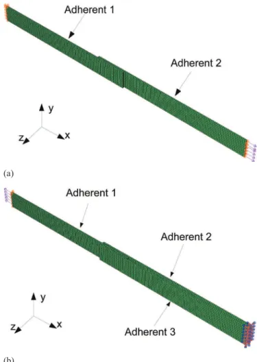
$¿QLWHHOHPHQWPRGHOIRUVLQJOHDQGGRXEOHODSMRLQWXVLQJ

commercial software ABAQUSTM _{was developed to compare}  WKH UHVXOWV WR WKH 6$- DQDO\VHV 7KH ¿QLWH HOHPHQW PRGHO

(single and double lap joint) uses a second­order hexahedron  element with 20 nodes (C3D20) for adherents, the adhesives  were modeled with a second­order hexahedron element with  20 nodes (C3D20) too. ABAQUSTM _{constraint function “tie” is} 

used to join the adhesive and adherents in the overlap region.  This  constraint  function  transfers  all  degrees  of  freedom 

EHWZHHQDGKHUHQWVDQGDGKHVLYH)LJXUHDVKRZVWKH¿QLWH

element model for single lap bonded joint and Fig. 5b shows 

WKH¿QLWHHOHPHQWPRGHOIRUGRXEOHODSERQGHGMRLQW

(a)

(b)

)RUWKH¿UVWVHWRIDQDO\VHVV\PPHWULFODPLQDWHFRPSRVLWH composite single and double lap bonded joints were investigated.  The adherent and adhesive mechanical properties and the joint  characteristics are shown in Table 1. A normal load in x direc­ tion of 1 N/mm was applied on single and double lap joint.  This load is small enough in order to avoid inelastic strains in  adherents or in adhesive. Also, all the stresses in the adhesive  layer will be divided by the applied stress (normalized stresses) 

in order to improve the comprehension of the load transfer by  the bonded joint.

)LJXUHDVKRZVWKHGLVSODFHPHQW¿HOGLQz direction for  single lap joint. It is possible to verify the difference between  UHVXOWV IURP 6$- DQG IURP RWKHU VRIWZDUH )RU WKH ¿QLWH element model, at the edge of adherent 1, all displacements  (x, y and zDUH¿[HGDQGDOOURWDWLRQVDUHIUHH)LJD,Q

the opposite edge, at adherent 2, zGLVSODFHPHQWLV¿[HGDOO

­80 ­60 ­40 ­20 0 20 40 60 80 100 ­1.0

­0.5 0.0 0.5 1.0

overall length (mm)

w

 (mm)

 ESAComp  SAJ  ABAQUS

­80 ­60 ­40 ­20 0 20 40 60 80 100

­0.0015 ­0.0010 ­0.0005 0.0000 0.0005 0.0010 0.0015

w

 (mm)

overall length (mm)

 ESAComp  SAJ  ABAQUS

(a)      (b)

0 5 10 15 20

­0.10 ­0.05 0.00 0.05 0.10 0.15 0.20 0.25

0.30  ESAComp Vz,   ESAComp Wzx  SAJ Vz,   SAJ Wzx

 ABAQUS Vz,   ABAQUS Wzx

Vz

, 

Wzx

 [

MPa

/MPa

]

"overlap" (mm)    

0 5 10 15 20

­0.06 ­0.04 ­0.02 0.00 0.02 0.04 0.06 0.08

Vz

, 

Wzx

[MPa

/MPa

]

"overlap" (mm)

 ESAComp V_z,   ESAComp W_zx  SAJ Vz,   SAJ Wzx

 ABAQUS Vz,   ABAQUS Wzx

(c)      (d)

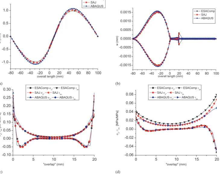
Figure 6. (a) Single lap composite joint displacement in w(z) direction; (b) double lap composite joint displacement in w(z) direction; (c)  normalized single lap joint ı_az and IJ_ax ; (d) normalized double lap joint ı_az and IJ_ax.

7DEOH 0HFKDQLFDO SURSHUWLHV DQG MRLQW FKDUDFWHULVWLFV +H[FHO77)FDUERQ ¿EHU UHLQIRUFHG SODVWLF +\VRO ($HSR[\ adhesive and aluminum/2024­T3 (Tita et al., 2008)

E₁ [kN/mm2_{] E} 2 [kN/mm

2_{] G}

12 [kN/mm

2_] Ȋ _{Thickness [mm] Orientation}

Hexcel T3T­190­F155 126.0 7.1 4.0 0.3 0.8 (0.2mm per ply) [0/45]s

Epoxy adhesive 1.485 ­ ­ 0.35 0.5 ­

rotations  are  free  and  the  loading  is  applied  in  x  direction  (Fig. 5a). For SAJ, at the edge of the adherent 1, x(u) and z(w) 

GLVSODFHPHQWVDUH¿[HGDQGURWDWLRQDWy(v) is free (Fig. 1a). In 

WKHRSSRVLWHHGJHDWDGKHUHQW]ZGLVSODFHPHQWLV¿[HG

rotation at y (v) is free and the normal loading is applied in  x(u) direction (Fig. 1a).

7KHERXQGDU\FRQGLWLRQVDSSOLHGIRU¿QLWHHOHPHQWPRGHO

and  SAJ  are  almost  the  same.  These  small  differences  are  due to limitations of the hypothesis adopted for SAJ and the  mathematical procedure used to solve the set of differential 

HTXDWLRQV7KXVWKHGLVSODFHPHQW¿HOGRI¿QLWHHOHPHQWPRGHO

is a little bit higher than SAJ, i.e. the SAJ model is slightly 

VWLIIHUWKDQ¿QLWHHOHPHQWPRGHO%RWK6$-DQG(6$&RPSTM 

do not regard for free edge effects on the adhesive layer.   It is important to mention that the commercial software  ESACompTM  _{has  some  limitations  of  boundary  conditions} 

once only three types of boundary conditions are available. In 

IDFWUHDOVWUXFWXUHVERXQGDU\FRQGLWLRQVDUHUDWKHUGLI¿FXOWWR EHVLPXODWHGWKXVVLPSOL¿FDWLRQVPXVWEHDVVXPHG'HVSLWH

SAJ  uses  the  same  set  of  equations  used  in  ESACompTM_,  WKLVFRPSXWDWLRQDOWRROLVPRUHÀH[LEOHWRVLPXODWHGLIIHUHQW

boundary conditions, but still has some limitations (for some  boundary  conditions  was  not  possible  to  solve  the  set  of  differential equations). Despite the limitations to apply bound­

ary conditions showed by ESACompTMDQG6$-LQWKH¿QLWH

element model is possible to simulate any boundary condi­ tions. So, in order to proceed with the analysis, the boundary  conditions  between  SAJ  and  ESACompTM  _{were  keep  as}  FORVHDVSRVVLEOHDVZHOODVIRUWKH¿QLWHHOHPHQWPRGHO7KH

ESACompTM _{boundary conditions are:}

x Simple Supported (SS): in this condition in one edge all the  displacements are restricted and in the other edge only the  vertical displacement is restricted. All the moments are free;

x Clamped­Free (CF): in this boundary condition one edge  is clamped (all displacements and rotations are restricted)  and the other edge is completely free;

x Clamped­Clamped  (CC):  this  condition  means  that  one  edge all the degrees of freedon are restricted and in the  other edge only the rotations are restricted.

  Due to ESACompTM _{limitations, the boundary conditions} 

used for simulations were similar to SS.

  The differences between SAJ and ESACompTM _responses 

(Fig. 6) are due to numerical differences to solve the set of  differential equations and small differences in the boundary 

FRQGLWLRQV)LJXUHDVKRZVWKHGLVSODFHPHQW¿HOGIRUWKH

entire single lap joint. The joint dimensions and coordinates  were  shown  in  Fig.  1a  for  single  lap  joint  and  Fig.  1b  for  double lap joint.

)LJXUHEVKRZVWKHGLVSODFHPHQW¿HOGIRUWKHHQWLUHGRXEOH ODSMRLQWDQGDOOUHVXOWVDUHYHU\FORVH)RUWKH¿QLWHHOHPHQW

model, in the edge of adherents 2 and 3, all displacements and 

URWDWLRQVDUH¿[HG)LJE,QWKHRSSRVLWHHGJHDWDGKHUHQW

only the loading is applied in x direction (Fig. 5b). For SAJ, in  the edge of the adherents 2 and 3, x(u) and z(w) displacements 

DUH¿[HGDQGDOOURWDWLRQVDUH¿[HG)LJE,QWKHRSSRVLWH

edge, at adherent 1, only the normal loading is applied in x(u)  direction (Fig. 1b). The same consideration for boundary condi­

WLRQVLVDSSOLHGWRWKLVFDVH7KXVWKHGLVSODFHPHQW¿HOGRI ¿QLWHHOHPHQWPRGHOLVDOLWWOHELWKLJKHUWKDQ6$-LHWKH6$-PRGHOLVVOLJKWO\VWLIIHUWKDQ¿QLWHHOHPHQWPRGHO

  Regarding to ESACompTM_{, the CF boundary conditions} 

were adopted which are, as for the last case, the most similar  boundary conditions available in the software to proceed with  the evaluations. In this case, despite the differences, the results  are very close to SAJ (Fig. 6).

  Figure 6c shows the normalized ı_az and IJ_ax for single lap  bonded  joint  and  all  results  are  again  similar  too.  In  this  case,  it  is  possible  to  observe  that  the  normal  stress  in  the  adhesive  layer ı_az  has  a  relatively  high  tensile  stress  in  the  adhesive edge, than it changes to compressive stress in less  than 2.5 mm and in 5.0 mm the normal stress is almost zero  or has a very low value. The same behavior is observed in  the  other  edge.  Equation  6  explains  this  behavior  (for  SAJ  and ESACompTM_{) once it regards the relative displacement}  EHWZHHQWKHDGKHUHQWV7KHVLQJOHODSMRLQW¿QLWHHOHPHQWDOVR

has the same behavior for normal stress in the adhesive layer.   Figure 6d shows that SAJ results of ı_az and IJ_ax for double lap 

MRLQWFRQYHUJHRQWKH¿QLWHHOHPHQWPRGHOUHVXOWV+RZHYHU

the ESACompTM _{results are different. These differences depend} 

are shown in Table 1. The boundary conditions and loading  for single and double lap joints were applied as commented  earlier.

)LJXUH D VKRZV WKH GLVSODFHPHQW ¿HOG IRU WKH HQWLUH single lap joint, where ESACompTMUHVXOWVDUHPRUHÀH[LEOH

in the composite side and stiffer in the aluminum side. SAJ  results  are  between  ESACompTMDQG¿QLWHHOHPHQWPRGHO

results.  This  occurs  due  to  differences  in  computational  method applied to solve the problem, as well as the boundary  FRQGLWLRQVDSSOLHG)LJXUHEVKRZVWKHGLVSODFHPHQW¿HOG for the entire double lap joint and the SAJ results converge to 

WKH¿QLWHHOHPHQWUHVXOWV+RZHYHUWKH(6$&RPSTM _results 

are different due to the applied boundary conditions. Figure  7c shows ıaz and IJax for single lap bonded joint and all results 

are very close. The stress singularity appears again for single  lap hybrid joint.

  For  double  lap  joint,  there  are  differences  between  the  results of ıaz and IJax (Fig. 7d). These differences depend on the 

applied boundary conditions, as well as the solution algorithm  used  in  each  model,  as  discussed  earlier.  It  is  important  to  note, again, that the highest differences are observed at the  end of the overlap region, where the highest stress values are 

YHUL¿HG7KHUHVXOWVIRU6$-DQG(6$&RPSTM _{are very similar,} 

EXWWKH¿QLWHHOHPHQWPRGHOUHVXOWVVKRZORZHUVWUHVVYDOXHV This occurs because SAJ and ESACompTM _{use a cylindrical} 

ÀH[XUDOK\SRWKHVLVDVGHVFULEHGE\0RUWHQVHQ   As commented before, the stress singularity that appears for  single lap joints (composite­composite or composite­metal) is  due to the relative displacements between the adherents (Eq.6).  Once the set of equations (Eqs. 2 and 3) regards the adhesive  stresses  they  affect  the  solution  and  then  in  the  adherents  kinematics. In the single lap joint solution, inside the overlap 

­80 ­60 ­40 ­20 0 20 40 60 80 100 ­1.0

­0.5 0.0 0.5 1.0 1.5 2.0 2.5 3.0 3.5

 ESAComp  SAJ  ABAQUS

Composite

w

 (mm)

overall length (mm)

Aluminum   

­80 ­60 ­40 ­20 0 20 40 60 80 100 ­0.0016

­0.0014 ­0.0012 ­0.0010 ­0.0008 ­0.0006 ­0.0004 ­0.0002 0.0000 0.0002 0.0004 0.0006 0.0008 0.0010 0.0012 0.0014 0.0016

 ESAComp  SAJ  ABAQUS

overall length (mm) Composite

w

 (mm)

Aluminum

(a)      (b)

0 5 10 15 20

­0.08 0.00 0.08 0.16 0.24 0.32 0.40 0.48 0.56

 ESAComp σ

z,   ESAComp τzx  SAJ σ

z,   SAJ τzx  ABAQUS σ

z,   ABAQUS τzx

σz

, 

τzx

[MPa

/MPa

]

"overlap" (mm)    

0 5 10 15 20

­0.08 ­0.06 ­0.04 ­0.02 0.00 0.02 0.04 0.06 0.08

0.10  ESAComp 

σ

z,   ESAComp τzx

 SAJ σ

z,   SAJ τzx

 ABAQUS σ

z,   ABAQUS τzx

σz

, 

τzx

[MPa

/MPa

]

"overlap" (mm)

(c)      (d)

Figure 7. (a) Single lap hybrid joint displacement in w direction; (b) double lap hybrid joint displacement in w direction; (c) normalized single 

region, the w displacement of adherent 2 (see Eq. 6) becomes  bigger (in absolute value) than the vertical displacement of  adherent 1. This behavior leads to a compressive normal stress  in the adhesive layer. Also it is important to mention that the  numerical procedures used in SAJ or in ESACompTM _smooth 

the  results  between  each  subdivision  avoiding  discontinu­

LW\IRUWKHVROXWLRQ7KHVLQJOHODS¿QLWHHOHPHQWPRGHODOVR VKRZVWKHVDPHEHKDYLRUIRUQRUPDOVWUHVVFRQ¿UPLQJWKDW

the  relative  displacement  between  the  adherents  leads  to  a  compressive normal stress close to the adhesive layer edges.   Considering  the  results  shown  earlier,  it  is  possible  to  conclude that SAJ is a computational tool, which can predict  the mechanical behavior of composite­composite and metal­ composite  bonded  joints  (single  and  double)  with  similar  accuracy  shown  by  other  software.  Therefore,  in  the  next  section, some design parameters will be investigated in order to 

VWXG\WKHLULQÀXHQFHRQWKHVWUXFWXUDOSHUIRUPDQFHRIERQGHG

joints.

Design  parameters  study  for  composite  bonded  joints  using SAJ

  One  of  the  most  important  components  of  the  joint  is  the adhesive layer at the overlap region, where physical and  chemical interactions between adherents and adhesive occur  and  the  load  is  transferred  from  the  part  (adherent)  to  the  adhesive  and  vice  versa.  Thus,  design  parameters  such  as  overlap length, type of joint, adhesive elastic modulus, and  adhesive  layer  thickness,  which  affect  the  stress  distribu­ tion in the overlap region, mainly the ıaz and IJax component  stresses,  were  investigated.  For  all  parametric  studies,  the  boundary conditions and loading were applied as described  here in section Evaluation of the computational tool (SAJ).  The mechanical properties and other important characteris­ tics for adhesive and adherents are given in Table 2 for both  types of joints (single and double).

Effect of the overlap length

  For this investigation, metal­composite single and double  lap  joints  were  used. A  load  of  1  N/mm  was  used  for  both  types of joints. Aluminum 2024­T3 was assumed in single lap 

MRLQWDVDGKHUHQWDQGIRUDGKHUHQWFDUERQ¿EHUFRPSRVLWH

(Hexcel T3T­190­F155). For the double lap joint, aluminum  2024­T3 was assumed for adherent 1, and composite mate­ rial was applied for other adherents. An epoxy adhesive was  considered for both types of joints.

  Figure  8a  shows  the  effect  of  the  overlap  length  in  the  adhesive  layer  stress  distribution  for  a  single  lap  joint  and  Figure 8b shows the results for double lap joint. Table 2 shows  the ıaz and IJax values obtained at the left edge of the adhesive  layer for single and double lap joint (Fig. 1). Based on the  results, it is observed that an increase in the overlap length  leads decreases of stress state in the adhesive edge, mainly 

Table 2.  Normalized maximum absolute stress values for various 

overlap lengths at the left edge of the adhesive layer

Single lap joint

Overlap length (mm) 15 20 25

ıaz 0.663 0.621 0.583

IJax 0.479 0.457 0.439

Double lap joint

Overlap length (mm) 15 20 25

ıaz 0.130 0.130 0.130

IJax 0.223 0.223 0.223

0 2 4 6 8 10 12 14 16 18 20 22 24 ­0.2

­0.1 0.0 0.1 0.2 0.3 0.4 0.5 0.6 0.7 0.8

Vz Wzx

[MPa

/MPa

]

"overlap" (mm)

 overlap=15mm (Vz)   overlap=15mm (Wzx)   overlap=20mm (Vz)   overlap=20mm (Wzx)  overlap=25mm (Vz)   overlap=25mm (Wzx)

(a)

0 2 4 6 8 10 12 14 16 18 20 22 24

­0.15 ­0.10 ­0.05 0.00 0.05 0.10 0.15 0.20 0.25

Vz Wzx

[MPa

/MPa

]

"overlap" (mm)

 overlap=15mm (Vz)   overlap=15mm (Wzx)  overlap=20mm (Vz)   overlap=20mm (Wzx)  overlap=25mm (Vz)   overlap=25mm (Wzx)

(b)

for single lap joints, considering the lengths studied in this  paper. Besides, the rate for stress reduction decreases with an  increase in the overlap length. So, it is possible to conclude  that  there  is  a  length  in  which  any  further  increases  in  the  overlap length do not decrease the stress state in the adhesive  layer edge. This trend is clearer for the double lap joint.

Comparison between single and double lap joints

  For  this  study,  all  the  joint  parameters  for  single  and 

double lap joint were kept the same as for the overlap effect  analysis.  It  is  important  to  note  that  the  overlap  length  is  equal 20 mm. The results are shown for half of the overlap  length in the region with greater differences between these  two types of joints.

  Figure 8 shows the difference between double and single 

lap joint stress distribution in the adhesive layer for the same 

load conditions and same joint characteristics. Figure 9a shows  the difference between these two types of bonded joints for 

shear stress in the zx­plane (IJax) and Fig. 9b shows the differ­

ence for the normal stress (ıaz). As expected, the amplitude 

range of ıaz and IJaxYDOXHVDUHVLJQL¿FDQWO\JUHDWHUIRUVLQJOH

lap joints.

Effect of the adhesive elastic modulus

  Another  important  parameter  is  the  adhesive  elastic 

modulus.  This  parameter  was  investigated,  keeping  other  parameters constant and using three realistic values for the  adhesive elastic modulus (1.5GPa; 2.0GPa; 3.0GPa) found in  the literature (San Román, 2005).

  Analysis of the effect of this parameter on the stress distri­

bution in the adhesive layer was performed. In this case study,  a normal load of 1 N/mm was imposed for both types of joints.  Figure 10a shows the results for single lap joint, and Fig. 10b  for double lap joint.

0 2 4 6 8 10

0.0 0.1 0.2 0.3 0.4 0.5

 Double Lap  Single Lap

Wzx

[MPa

/MPa

]

"overlap" (mm)

(a)

0 2 4 6 8 10

­0.2 ­0.1 0.0 0.1 0.2 0.3 0.4 0.5 0.6

σz

[MPa

/MPa

]

"overlap" (mm)

 Double Lap  Single Lap

(b)

Figure 9. Single vs. double lap joint (half of the overlap length): (a) 

normalized IJ_zx

 shear stress in plane zx; (b) normalized ız  normal stress in z direction.

0 5 10 15 20

­0.15 ­0.10 ­0.05 0.00 0.05 0.10 0.15 0.20 0.25 0.30 0.35 0.40 0.45 0.50

 E=1,5 GPa (σ

z)   E=1,5 GPa (τzx)

 E=2,0 GPa (σ

z)   E=2,0 GPa (τzx)

 E=3,0 GPa (σ_z)   E=3,0 GPa (τ_zx)

σz ,τz

x

[MPa

/MPa

]

"overlap" (mm)

(a)

0 5 10 15 20

­0.10 ­0.08 ­0.06 ­0.04 ­0.02 0.00 0.02 0.04 0.06 0.08 0.10 0.12

σz ,τz

x

[MPa

/MPa

]

"overlap" (mm)  E=1,5 GPa (σ

z)   E=1,5 GPa (τzx)

 E=2,0 GPa (σ

z)   E=2,0 GPa (τzx)

 E=3,0 GPa (σ

z)   E=3,0 GPa (τzx)

(b)

  It can be observed that adhesives with lower values of elas­ tic modulus lead to lower stress state in the overlap region for  single and for double lap bonded joints. This can be explained  E\(TVDQG+RZHYHUPRUHÀH[LEOHDGKHVLYHVKDYH low strength values, and in a real joint design, it is desirable that  the adhesive has a satisfactory performance. Thus, it is impor­ tant to balance the stiffness and the strength of the adhesive  layer. Besides, the adhesive can show inelastic strains according  to the level of loading and the yielding stress of the polymer.

Effect of the adhesive layer thickness

  The  adhesive  layer  thickness  affects  the  stress  distribu­ tion in the adhesive layer. This parameter was investigated,  keeping the other parameters constant, regarding three real­ istic adhesive layer thicknesses (0.05 mm; 0.5 mm; 1.0 mm),  which are found in the literature (Qian and Sun, 2009). The  mechanical properties and composite adherents and adhesive  characteristics  are  shown  in  Table  1.  The  analyses  were 

carried out using a normal load of 1 N/mm. This load leads  to adhesive stresses low enough to avoid adhesive non­linear  behavior, or any adhesive or adherent failure.

  Figure  11a  shows  a  single  lap  joint  adhesive  stresses  distribution for three different thicknesses, and Fig. 11b for  double lap joint. These results show that this parameter can  VLJQL¿FDQWO\ DIIHFW WKH DGKHVLYH OD\HU VWUHVV GLVWULEXWLRQ mainly  close  to  the  edge  of  the  overlap  region. Adhesives  with lower values of thickness lead to higher stress state in  the overlap region for single and for double lap bonded joints.  This can be explained by Eqs. 4, 5 and 6.

CONCLUSIONS

  SAJ, a new computational tool, has shown to be adequate in  performing composite­composite and metal­composite single  and double bonded joint analysis. Therefore, very quickly, it  is possible to analyze a set of different joints, varying many  parameters, for example: materials (adhesives and/or adher­ HQWV¿EHURULHQWDWLRQDQGVWDFNLQJVHTXHQFHRIWKHODPLQDWH thickness of the laminate and/or the adhesive; overlap length  and the type of the joint (single or double). However, due to  WKH F\OLQGULFDO ÀH[XUDO K\SRWKHVHV WKH FRPSXWDWLRQDO WRRO provided some small deviations in the results, when compared  WR¿QLWHHOHPHQWDQDO\VHV,QUHJDUGVWRVWUHVVGLVWULEXWLRQ6$-UHVXOWLQJYDOXHVDUHJUHDWHUWKDQ¿QLWHHOHPHQWDQDO\VHV7KXV the analyses from SAJ are more conservative, which is very  interesting for conceptual and preliminary design of a product.   Regarding to parametric study, SAJ leads to some conclu­ sions, which can be used as a guide during product design. For  example,  a  thicker  adhesive  layer  (keeping  other  parameters  constant) could reduce the adhesive edge stress state, increas­ ing the strength of the joint, but thicker adhesives could lead  to  adhesive  cohesive  failure.  The  adhesive  stiffness  affects  WKHVWUHVVVWDWHDQGDPRUHÀH[LEOHDGKHVLYHUHGXFHVWKHVWUHVV peak at the edges of the adhesive layer. Therefore, it is more  UHFRPPHQGDEOHWRXVHPRUHÀH[LEOHDGKHVLYHV+RZHYHUPRUH ÀH[LEOHDGKHVLYHVQRUPDOO\KDYHORZHUVWUHQJWKYDOXHV7KXV it is important to verify what is more important to the product  in service. Short overlap length increases the stress peak at the  adhesive layer edges. Thus, it is reasonable to increase the over­ lap length, but the joint weight could increase too. Therefore,  it is very important to balance all parameter values. Finally, by  understanding the behavior of the stress distribution in the joint,  it is possible to design products made of bonded joints with more  accuracy even during the conceptual and preliminary phases.

0 5 10 15 20

­0.2 0.0 0.2 0.4 0.6 0.8

Vz Wzx

[MPa

/MPa

]

"overlap" (mm)  t=0,05mm (Vz)   t=0,05mm (Wzx)

 t=0,50mm (Vz)   t=0,50mm (Wzx)

 t=1,00mm (Vz)   t=1,00mm (Wzx)

(a)

 t=0,05mm (Vz)   t=0,05mm (Wzx)

 t=0,50mm (Vz)   t=0,50mm (Wzx)

 t=1,00mm (Vz)   t=1,00mm (Wzx)

0 5 10 15 20

­0.25 ­0.20 ­0.15 ­0.10 ­0.05 0.00 0.05 0.10 0.15 0.20 0.25 0.30 0.35

Vz Wzx

[MPa

/MPa

]

"overlap" (mm)

(b)

REFERENCES

Agnieszka, D., 2009, “Prediction of the failure metal­compos­ ite bonded joints”, Computational Materials Science, Vol. 45,  No. 3, pp. 735­738.

Belhouari, M. et al._{, 2004, “Comparison of double and single} 

bonded repairs to symmetric composite structures: a numeri­ cal analysis”, Composite Structures, Vol. 65, No. 1, pp. 47­53.

Butcher, J.C., 2003, “Numerical Methods for Ordinary Differ­ ential Equations”, New York, John Wiley & Sons.

Charalambides, M.N. et al._{, 1998, “Adhesively bonded repairs} 

WR¿EUHFRPSRVLWHPDWHULDOV,,)LQLWHHOHPHQWVPRGHOLQJ´ Composites – Part A, Vol. 29, pp. 1383­1396.

Frostig, Y. et al._{, 1997, “Analysis of adhesive bonded joints,} 

VTXDUHHQGDQGVSHZ¿OOHWFORVHGIRUPKLJKHURUGHUWKHRU\ approach”, Report No. 81, Institute of Mechanica1 Engineer­ ing, Aalborg University, Denmark.

Ganesh,  V.K.  and  Choo,  T.S.,  2002,  “Modulus  graded  composite adherents for single lap bonded joints”, Journal of  Composite Materials, Vol. 36, pp. 1757­1767.

Goland, M. and Reissner, E., 1944, “The stresses in cemented  joints”, Archive of Applied Mechanics. Vol. 11, pp. A17­A22.

Goyal, V.K. et al._{, 2008, “Predictive strength­fracture model} 

for composite bonded joints”, Composite Structures, Vol. 82,  No. 3, pp. 434­446.

Hart­Smith, L.J., 1973, “Adhesive­bonded scarf and stepped  joints”. Washington, DC, NASA, (NASA CR11223).

Hart­Smith,  L.J.,  1970,  “The  strength  of  adhesive­bonded  single­lap joints”, Santa Monica, Douglas Aircraft Company,  IRAD Technical Report Number MDC­J0742.

Kim, T.H. et al._{, 2008, “An experimental study on the effect} 

of  overlap  length  on  the  failure  of  composite  to  aluminum  single lap bonded joints”, Journal of Reinforced Plastic and  Composites, Vol. 27, No.10, pp. 1071­1081.

Mortensen, F., 1998, “Development of Tools for Engineering  Analysis and Design of High­Performance FRP­Composite  Structural Elements”. Ph.D. Thesis, Institute of Mechanical  Engineering, Aalborg University, Aalborg.

Qian, H. and Sun, C.T., 2009, “Effect of bondline thickness on  model I fracture in adhesive joints” in SDM 2008: Proceedings  of the 49rd AIAA/ASME/ASCE/AHS/ASC Structures, Structural  Dynamics, and Materials Conference, Schaumburg, Illinois, USA.

Ribeiro, M.L. et al._{, 2010, “Development of a computational} 

tool for bonded joint analysis” in PACAM XI: Proceedings of  the 11th Pan­American Congress of Applied Mechanics, Foz  do Iguaçu, Brazil.

Saha,  G.  and  Banu,  S.  (2007),  “Buckling  load  of  a  beam­ column  for  different  end  conditions  using  multi­segment  integration technique”, Journal of Engineering and Applied  Sciences, Vol. 2, No. 1, pp. 27­32.

San Román, J.C., 2005, “Experiments on epoxy, polyurethane  and adhesives”, Composite Structure Laboratory, Technical  Report, CCLab2000.1b/1, Lausanne, Swiss.

Seong, M.S. et al._{, 2008, “A parametric study on the failure of} 

bonded single­lap joints of carbon composite and aluminum”,  Composite Structures, Vol. 86, pp. 135­145.

Shampine L. et al._{, 2006, Solving Boundary Value Problems} 

for Ordinary Differential Equations in MATLAB with bvp4c.  ACM Transactions on Mathematical Software, Vol. 31, No. 1,  pp. 79­94.

Silva, L.F.M. et al._{, 2009a, “Analytical models of adhesively} 

bonded joints­Part I: Literature survey”, International Journal  of Adhesion & Adhesives, Vol. 29, pp. 319­330.

Silva, L.F.M. et al._{, 2009b, “Analytical models of adhesively} 

bonded joints­Part II: Comparative study”, International Jour­ nal of Adhesion & Adhesives, Vol. 29, pp. 331­341.

Thomsen, O.T., 1992, “Elasto­static and elasto­plastic stress  analysis of adhesive bonded tubular lap joints”, Composite  Structures, Vol. 21, pp. 249­259.

Tita, V. et al.,2008, Failure analysis of low velocity impact  on  thin  composite  laminates:  Experimental  and  numerical  approaches. Composite Structures, v. 83, pp. 413­428. ;LDRFRQJ+³$UHYLHZRI¿QLWHHOHPHQWDQDO\VLVRI adhesively bonded joints”, International Journal of Adhesion  and Adhesives, Vol. 31, No. 4, pp. 248­264. Yuceoglu, U. and Updike, D.P., 1975, “The effect of bending  on the stresses in adhesive joints”, Lehigh University, Bethle­ hem, Pensylvania (NASA). Zarpelon, F.L., 2008, “Evaluation of Analytical Models for  Bonded  Repairs  of  Laminate  Composite”.  Dissertation,  Technological Institute of Aeronautics, São José dos Campos,  Brazil (in Portuguese).

APPENDIX I

For  Multiple  Point  Segment  Method,  consider  the  linear  differential equations system in matrix notation

( ) ( ) ( ) ( )

dx d

y x =A x $y x +B x

6 @   (7)

  y x (8)

y y y Where: m 1 2 g = ^ h R T S S S S S V X W W W W W

  , (9)

A a a a a a a a a a B b b b m m m m mm m 11 21 1 12 22 2 1 2 1 2 g g g g g g g g = = R T S S S S S R T S S S S S V X W W W W W V X W W W W W The boundary conditions could be described as:

Cy a^ h+Dy b^ h=E  (10)

The solution can be regarded as:

y x_{^ h=}Y x_{^ h}$G₊Z x_{^ h  (11)}

Where: G is the integration constant, Y(x) is the general solu­ tion of the system and Z(x) is the particular solution. Consider: . dx d

Y x_{^ h} =A x Y x_{^ h ^ h} withY a_{^ h}=I

6 @   (12)

( ) 0

dx d

Z x^ h =A x^ h$Z x^ h+B x^ h withZ a =

6 @   (13)

Solving the equation in x = a:

( ) .

y a =Y a^ h$G+Z a^ h  (14)

Solving  equation  14  in x=a,  yield G=Y(a)  and  for x=b  . 

Applying this results in (10), yields

( ) ( )

y a C D Y b 1 E D Z b

$ $ $

= + ‐ ‐

^ h

6 @ 6 @  (15)

Saha and Banu (2007) showed other example of the multiple  point segment method application.

APPENDIX II

  For the Matlab function “bvp4c”, consider a differential 

equation y"+ y = 0 smooth in the [a,b]. The boundary condi­

tion  in x  = a  is y(a) = A  and y’(a)  = s,  the  solution  of  the 

GLIIHUHQWLDOHTXDWLRQKDYHWR¿QGWKHYDOXHRIy(b,s) = %.

  Consider that the algebraic equation s has a solution. Regard 

a function u(x) as the solution for y(a) = A and y'(a) = 0 and v(x) 

be the solution for y(a) = 0 and y'(a) = 1, this linear approach  yields in y(x,s) = u(x) + sv(x) and with the boundary condition 

%= y(b,s) = u(b) + sv(b), its results in a linear set of algebraic 

linear equations with initial derivative equal s.

  In  some  kind  of  problems,  the  equations  to  solve  the 

problem are non­linear. It implies that the existence and the  XQLTXHQHVVRIWKHUHVXOWVDUHYHU\GLI¿FXOWSUREOHPWRVROYH

  In practice, to solve a set of differential non­linear equa­

tions are based in the solution of initial value problem and 

in non­linear equations solvers. MatlabTM _{“bvp4c” function} 

uses the colocation method to solve the problem. For example,  consider the following differential equation:

' , , ,

y =f x y p^ h a#x#b   (16)

  And the non­linear boundary conditions in x = a and x = b are:

, ,

g y a y b p^ ^ h ^ h h=0  (17)

  Where p is the vector of unknown parameters. The approxi­

mate solution, S(x), is a third order polynomial function smooth  in the interval [x_n, x_n+1] with mesh a = x₀ < x₁< … < x_n < b,  satisfying the boundary condition  g(S(a), S(b)) = 0 the interval  limits as well as the differential equations inside the mesh.   (18) ' , ' , ' ,

S x f x S x

S x x f x x S x x

S x f x S x

2 2 2

n n n

n n n n n n

n n n

1 1 1

1 1 1