NUCLEI SHELLS AND PERIODIC TRENDS. PART 2. Ядерные оболочки и периодический закон Д.И.Менделеева. Часть 2.

(1)

http://ej.kubagro.ru/2012/07/pdf/37.pdf

УДК 531.9+539.12.01 UDC 531.9+539.12.01

ЯДЕРНЫЕОБОЛОЧКИИПЕРИОДИЧЕСКИЙ

ЗАКОНД.И.МЕНДЕЛЕЕВА. ЧАСТЬ 2.

NUCLEI SHELLS AND PERIODIC TRENDS. PART 2.

Трунев Александр Петрович к.ф.-м.н., Ph.D.

Alexander Trunev

Cand.Phys.-Math.Sci., Ph.D.

Директор, A&E Trounev IT Consulting, Торонто, Канада

Director, A&E Trounev IT Consulting, Toronto, Canada

На основе теории ядерных взаимодействий и данных по энергии связи нуклонов для всех известных нуклидов установлены параметры, характеризующие периодические закономерности в формировании ядерных оболочек

Parameters describing periodic trends in the formation of nuclear shells have been established based on the theory of nuclear interactions and data on the binding energy of nucleons for the set of known nuclides

Ключевые слова: НЕЙТРОН, ПЕРИОДИЧЕСКИЙ ЗАКОН, ПРОТОН, ЭНЕРГИЯ СВЯЗИ, ЯДРО

Keywords: BINDING ENERGY, PERIODIC TRENDS, PROTON, NEUTRON, NUCLEI

Introduction

The periodic law discovered by Mendeleev in 1869, played a huge role in the

development of ideas about the structure of matter. In one of the first formulations

of this law states that "the properties of simple bodies, as well as the shape and

properties of the compounds of the elements, and therefore the properties of which

they form simple and complex bodies are in the periodic table according to their

atomic weight" [1]. Using this law, Mendeleev created the periodic table of

elements, which is predicted on the basis of new elements - gallium, scandium,

germanium, astatine, polonium, technetium, rhenium, and francium.

Ivanenko [2-3], evidently, was one of the first who raised the issue of

expansion of the periodic law to include the periodic patterns are observed in

atomic nuclei and some exotic formations, such as exotic atoms. According to the

theory of nuclear shells [4-5], periodic patterns in the nuclei are explained by

analogy with the electron shells, the Pauli principle, which is applied separately for

protons and neutrons fill the nuclear envelope. With this expansion of the periodic

law of its original wording seems quite logical, since the properties of the nuclei

(2)

Thus, the properties of nuclei and the properties of atoms of chemical elements due

to the same type on the basis of quantum mechanics and the Pauli principle.

At present, the binding energy of the nucleon measured with high accuracy

for almost all known nuclides. However, in contrast to the ionization energy of the

atoms, the dependence of the binding energy of the number of nucleons does not

contain any explicit reference to the existence of nuclear shells. However, attempts

to establish the presence of known nuclear shells and the so-called magic numbers

for the deviation from the standard binding energy trend of the Weiszäcker’s

semi-empirical model [6] and other models [7]. In the present work we investigated the

dependence of the energy of the nucleons for all known nuclides with the use of

Wolfram Mathematica 8 [8] and three models of the binding energy:

1) Semi-empirical model;

2) 5D model of nuclear interactions [9-11];

3) Information model [12].

The parameters of all models were determined locally for the isotopes of

each element. Found that in all three cases, model parameters have a similar

behavior depending on the number of protons, which indicates the presence of the

internal structure of nuclei.

5D model description

You may notice that the periodic law in the original formulation of

Mendeleev is local, as relates properties of simple substances with their atomic

weight, which at the time when the law was formulated, was determined by

weighing in the gravitational field of the earth. Such a correlation properties of

substances and their gravitational properties are reasonable. To answer the question

about the fundamental causes that lead to a law of periodicity in nature, consider a

general model of atomic nuclei and atoms of matter [10-11]. In this model, the

(3)

5-http://ej.kubagro.ru/2012/07/pdf/37.pdf

dimensional space, which depend on a combination of charge and gravitational

properties of the central core in the form [9]

2 2

4 2 3

/ 2 / ,

/

2 M c Q k M c

k = γ _A ε = γ _A (1)

Here γ,c,Q_{- the gravitational constant, the speed of light and charge of the}

nucleus, respectively. About the nature of the charge will be assumed that the

source is an electric charge, but it can be screened in various natural fields. The

mechanisms of screening and related fields are discussed below. In the case of

proton and electron parameters of the metric tensor (1) are presented in Table 1.

Table 1: The metric tensor parameters

k, 1/m ε rmax, m rmin, m e- 1,703163E-28 4,799488E-43 5,87E+27 2,81799E-15 p+ 1,054395E-18 1,618178E-36 9,48E+17 1,5347E-18

Note that the maximum scale rmax =1/k in the case of an electron exceeds the

size of the observable universe, while for protons this scale is about 100 light-years.

The minimum is the scale rmin = ε/k=e2/mc2 corresponds to the classical radius of a

charged particle, which in the case of a proton and an electron is commensurate

with the scale and the weak nuclear interactions.

It is easy to see that the second parameter of the model (1) directly included

in the formula for the Mendeleev’s periodic law [1]. Combining the parameters, we

find the nuclear charge in the form: Q =ε3/2c2 /k 2γ . Consequently, the

periodic law in its present formulation can also be expressed through the

parameters of the metric tensor (1). The metric tensor can be expanded in the

vicinity of a massive center of gravity in five-dimensional space in powers of the

dimensionless distance to the source, ~r =kr_{, here}

_r

=

_x

2

+

_y

2

+

_z

2 _.

Consider the form of the metric tensor, which arises when holding the first three

(4)

gravitational potential in the Newton’s form. This choice of metric is justified,

primarily because of the specified building the superposition principle holds.

Suppose x1=ct , x2= x , x3= y , x4=z_{, in this notation we have for the square of the}

interval in the 4-dimensional space:

r M dz dy dx c dt c c ds γ ϕ ϕ ϕ − = + + − − +

=(1 2 / 2) 2 2 (1 2 / 2)( 2 2 2) 2

(2)

Assuming that ε2 /k = 2γM /c2 _{we arrive at the expression of the interval}

depending on the parameters of the metric in the five-dimensional space:

) )( / 1 ( ) / 1

( 2 2 2 2 2 2 2

2 dz dy dx k dt c k

ds = −ε − +ε + + (3)

Further, we note that in this case the metric tensor in four dimensions is

diagonal with components

) / 1 ( ; /

1 2 ₂₂ ₃₃ ₄₄ 2

11 kr g g g kr

g = −ε = = =− +ε ₍₄₎

We define the vector potential of the source associated with the center of

gravity in the form

g1 = ε /kr, g=g1u (5)

Here u _{is a vector in three dimensional spaces, which we define below.}

Hence, we find the scalar and vector potential of electromagnetic field

ϕ = = ε , A=ϕ_eu

2 kr e Mc r Q

e (6)

To describe the motion of matter in the light of its wave properties, we

assume that the standard Hamilton-Jacobi equation in the relativistic mechanics and

the Klein-Gordon equation in quantum mechanics arise as a consequence of the

wave equation in five-dimensional space [9]. This equation can generally be

written as: 0 1 =       _Ψ ∂ ∂ − ∂ ∂

− µ µν ν

x G G x

(5)

Here Ψ - the wave function describing, according to (7), the scalar field in

five-dimensional space; ik

G _{- the contravariant metric tensor,}

                − − − − − − − − = − λ λ λ λ λ η 4 3 2 1 4 2 3 2 2 2 1 1 1 0 0 0 0 0 0 0 0 0 0 0 0 g g g g g g g g

Gik ₍₈₎

4 2 4 3 2 3 2 2 2 1 1 1 1 2 2 1 2 1 , , , ) / 1 ( ; ) / 1 ( g g g g g g g g kr kr λ λ λ λ ε λ ε λ = = = = + − = − = − − 2 3 5 2 4 2 3 2 2 2 2 1

1 ( ); /( ); ( )

1+ g + g +g +g G = ab = kr

= λ λ η η

λ _.

We further note that in the investigated metrics, depending only on the radial

coordinate, is true the following relation

(

)

(

µν

)

µ µν

µ

µ _η _η

G G dr d x r G G x F − ∂ ∂ = − ∂ ∂

= ₍₉₎

Taking into account the expressions (8) and (9), we write the wave equation

(7) as 2g 0 2 2 2 2 2 2 2 2 1 ₌ x Ψ F + ρ x Ψ ρ Ψ λ + Ψ | | t Ψ c μ μ i i ∂ ∂ ∂ ∂ ∂ − ∂ ∂ ∇ − ∂ ∂ _λ λ (10)

Note that the last term in equation (10) is of the order η2k=k5r4 <<1_.

Consequently, this term can be dropped in the problems, the characteristic scale

which is considerably less than the maximum scale in Table 1. Equation (10) is

remarkable in that it does not contain any parameters that characterize the scalar

field. The field acquires a mass and charge, not only electric, but also strong in the

process of interaction with the central body, which is due only to the metric of

5-dimensional space [9-11].

Consider the problem of the motion of matter around the charged center of

gravity, which has an electrical charge and strong, for example, around the proton.

(6)

matter and energy ties. Since equation (10) is linear and homogeneous, this

problem can be solved in general.

We introduce a polar coordinate system (r,φ,z) _{with the z axis is directed}

along the vector potential (8), we put in equation (10)

) exp(

)

( φ ω ρ

ψ r il +ikzz−i t−ikρ

=

Ψ (11)

Separating the variables, we find that the radial distribution of matter is

described by the following equation (here we dropped, because of its smallness, the

last term in equation (10)):

0 2

2g

1 2 2 1 1

2 2

2

1 _c _k _g _k _k ₌

λk k r l r | | c z z z r

rr ψ ψ ψ ψ ω ψ ψ

ψ λ ψ ω λ ρ ρ

ρ + −

−     − − + − − − (12)

Consider the solutions (12) in the case when one can neglect the influence of

gravity, i.e. λ₁ ≈ λ− ₂ ≈1_but λ=1+g₁2(1−u2)≠1_{. Under these conditions, equation}

(16) reduces to

0 2

2g

1 2 2 1 1

2 2 2 2 = k k g k c λk k r l r c z z z r

rr ψ ψ ψ ψ ω ψ ψ

ψ ψ ω

ρ ρ

ρ + −

−     ₊ ₋ ₋ − − − (13)

In general, the solution of equation (13) can be represented in the form of a

power series [10-11]

∑

=

−

=

n j j j

a

c

r

0

~

)

~

exp(

ψ

(14)

It is indicated r~ = r / rn . Substituting (14) in equation (13), we find

0 ~ ) 1 ( ~ 2 ~ ~ ) 1 ( ~ ) 1 2 ( ~ ) ( 0 2 0 2 0 1 0 2 2 2 2 0 1 0 2 2 2 = − + − − + − + + − + + −

∑

= − = − = − = = − = − n j j j n j j j n j j j n j j j n n z n j j j n g n j j j u r j j c r jc a r jc r c r K r k r c r a r c l

a κ κ

(7)

http://ej.kubagro.ru/2012/07/pdf/37.pdf 2 2 2 2 / ) 1

( u k k

u ε

κ = − ρ , K2 =kρ2 +ω2/c2, κg =−2εkρ(kzuz +ω/c)/k>0.

Hence, equating coefficients of like powers, we obtain the equations relating

the parameters of the model in the case of excited states

0

1 ,

2

1 ,

₂ 2 2 2 2

2

−

=

+

−

+

=

c

k

r

a

n

r

l

a

_z n g n u

ω

κ

_ρ (16)

The second equation (16) holds only for values of the exponent, for which

the inequality 2a <n+1_{is true. Hence, we find an equation for determining the}

energy levels

0 )

2

1 (

4

2 2 2 2 2 2 2 2 2

=

+

−













₊

−

+

a

k

u

c

k

c

n

k

z z z

ω

ε

ρ ρ (17)

Equation (17) was used to model the binding energy of nucleons in the

nucleus for the entire set of known nuclides [10-11]. In the model [10-11], the core

consists of "pure" proton interacting with a scalar field. Part of the "pure" proton is

screened by forming N neutrons, as a result there is an atom, consisting of the

electron shell and nucleus with electric charge eZ, number of nucleons

N Z

A = + _,_{mass excess} ME = M − A_{, and the binding energy}

MeV C m m m A ME Nm m m Z E u u n p e b 494028 . 931 12 / ) ( ), ( ) ( 12 ≈ = ⋅ + − + + =

Note that we using the standard expression of the mass excess in atomic

units. Since two types of charges - scalar and vector, appear in this problem the

effect of screening manifests itself not only with respect to the scalar charge (which

leads to the formation of neutrons), but also in terms of the vector of the charge,

which leads to the formation of the nucleons.

It should be noted that the original metric in the five-dimensional space

(8)

body, i.e. of the total charge and total mass of the nucleons. Different shells can be

formed depending on the combination of the charge and mass of the nucleus:

1) Nucleon shell, in which all charges are screened,

thereforeε /k== A2e2/Am_pc2 = Ae2/m_pc2_;

2) Neutron shell, in which we have ε/k = Ne2/m_pc2_;

3) Proton shell, in whichε /k =Ze2/m_pc2_.

Using the electron mass and Planck's constant, we define the dimensionless

parameters of the model in the form

2 2 2 2 , , ) ( ) ( , c m E c m k P c m k S c e e e z e ω

α h ρ h h

h = = =

=

(

)

2

2 2 2 2 2 2 ) / ( ) 1 ( 2 1 ) / ( 4 p e p e X nl m m SX u l n m m X b α α − − − +

= ₍₁₈₎

Here X = A,N ,Z in the case of the nucleon, neutron and proton shells,

respectively.

Solving equation (17) with respect to energy, we find

) 1 ( ) )( 1 ( )

( 2 2 2 2

+ + − + + − ± − = _X nl X nl X nl X nl X nl X nl Sb u P Sb P S Sb Pu Sb i Pu Sb

E (19)

Note that the parameter in the energy equation (19) can be both real and

complex values, which correspond to states with finite lifetime. Given that for most

nuclides the decay time is large enough quantity; it can be assumed that the

imaginary part of the right-hand side of equation (19) is a small value, which

corresponds to a small value of the radicand. Hence we find that for these states the

following relation between the parameters

) 1 ( 1 ) 1 ( 2 2 u Sb Sb S P _X nl X nl − + +

= ₍₂₀₎

(9)

http://ej.kubagro.ru/2012/07/pdf/37.pdf )) 1 ( 1 )( 1 ( 2 2 / 3 u Sb Sb u b S E X nl X nl X nl X nl − + +

= ₍₂₁₎

Hence, we find the dependence of the binding energy per nucleon in the

ground state )) 1 ( 1 )( 1 ( / / 2 2 0 2 0 2 0 2 / 3 0 u X Sb X Sb A uX b S A EX a − + +

= ₍₂₂₎

It is indicated b0 = (2αme /mp(1− 2a))2 . Thus, we have established a link

the energy of the state parameters with the interaction parameter. Note that the

energy of ground state (22) depends on the magnitude of the vector charge, which

appears in equations (5) - (6). In [11] have shown that this shows the difference

between the interaction of nucleons in nuclei, where the parameteru ≠ 0_{, and the}

interaction between electrons and atomic nuclei, in whichu = 0 _.

Equation (22) allows us to describe the dependence of the binding energy of

the number of nucleons for all nuclides. The computational model is constructed as

follows. Suppose that, based on equation (22) was able to accurately determine the

binding energy of one of the isotopes of an element. Without loss of generality we

can assume that this is isotope, which contains the minimum number of neutrons.

Then the binding energy of all other isotopes of element is defined by

min min 0 0 min min

0 ( , ) ( , ) ( , )

) , ( N Z Z N E N Z Z N E N Z Z N E A Z N

E Na

N a A a + − + + +

= ₍₂₃₎

Model (23) contains the arbitrary choice of the interaction parameterSb0 .

Further, without loss of generality we assume that Sb0 = 1 , therefore a momentum

scale in the fifth dimension appearing in equations (11) - (17) is established.

Computation of the binding energy of nucleons

We consider three models of the binding energy of nucleons. Standard

(10)

4 / 3 5 1 2 3

/ 1 2 3

/ 2

)

( − −

− ₋ ₋ ₊

− −

= a A a A a Z A a N Z A a A

E_b _v _s _c _A (24)

The first term on the right side of (24) describes the increase in binding

energy due to the increase in the volume of the system, the second term is due to

the contribution of surface energy, the third term describes the contribution of the

electric charge of protons, the fourth term due to the contribution of the Fermi

energy of nucleons, and finally, the fifth term describes the pairing energy. Since

the model (24) depends on five parameters, and model (23), only three, we fix two

parameters in equation (24). First, we assume as = 17.23 that is consistent with

the known data [6]. Second, we assume a5 = 0 that due to the specifics of the

problem, in which the model parameters are defined locally for a given value of the

nuclear charge, and in this case there is no sufficient data to determine this

parameter. Consequently, it is necessary to determine the three parameters of the

modelav,ac,aA, depending on the number of protons Z.

5D model of the binding energy (23) depends on three parameters. For a

given number of protons can be represented as

) ) ( 1 )( 1 (

/ /

2 2

2

gN k N

A bN a

A E_b

+ + +

= ₍₂₅₎

The problem is to find the values of model parameters (25) a,b,g ,

depending on the number of protons Z.

The information model is based on the binding energy changes in terms of

energy of a thermodynamic system

PdV TdS

dE = −

We can assume that in the case of core contributions of pressure and volume

is described by the first term on the right side of equation (24), and entropy of the

system varies with the number of neutrons, like the entropy of a discrete set [12],

(11)

) ) / ln( )( / (

/A a1 b1 N A N A g1

Eb = + − + (26)

Note that in the system Mathematica 8 [8] has built a database of isotopes

IsotopeData [], and the procedure for finding the parameters of linear and nonlinear

models - Fit, FindFit, NonlinearModelFit. The coefficients of the three models (24)

- (26) were calculated in the system [8] for the isotopes of chemical elements

(Appendix B shows an example for the model (24)). Model (25) is rigid, so in the

calculation of its parameters is introduced numerical coefficient k, which provides

the convergence of the solution (see example below in Appendix section). Model

(26) can be used without change, but in some cases, a sign in front of the logarithm

should be replaced with the opposite sign on the initial iteration. Three models can

be compared with experimental data (the corresponding code shows in the

Appendix). Results comparing the three models are shown in Figure 1 for isotopes

of O, F, Fe, Ni, Pt, Au curves of different colors - green, red and blue for models

(24), (25), (26), respectively.

Parameters of the three models, calculated for the number of protons from 4

(12)

Figure 1: Comparison of three models for the isotopes O, F, Fe, Ni, Pt, Au:

the green lines – Weiszäcker’s model (24), red lines - 5D model (25), blue lines -

an information model.

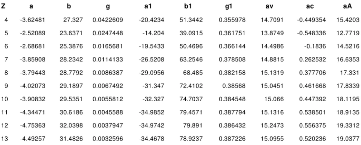
Table 2: The calculated parameters of models (24) (25) and (26).

Z a b g a1 b1 g1 av ac aA

(13)

(14)

57 -6.71471 34.8831 0.0001287 -51.7677 105.403 0.439024 15.5096 0.688154 22.5647 58 -6.77462 34.9917 0.0001243 -51.8113 105.447 0.43912 15.4913 0.682866 22.5949 59 -6.61779 34.5162 0.0001194 -50.9097 103.723 0.439992 15.4053 0.669129 22.2552 60 -6.64243 34.5196 0.0001151 -51.3111 104.33 0.440713 15.414 0.669337 22.3221 61 -6.5384 34.155 0.0001105 -50.6191 102.949 0.441853 15.3515 0.660245 22.0511 62 -6.571 34.1944 0.0001069 -50.5155 102.727 0.442029 15.3256 0.654196 22.0297 63 -6.54571 34.0061 0.0001026 -50.1268 101.863 0.44335 15.2915 0.650338 21.8645 64 -6.60085 34.0906 9.923E-05 -51.0797 103.449 0.443885 15.3239 0.654754 22.0742 65 -6.50471 33.7317 9.524E-05 -50.3913 102.047 0.445361 15.272 0.647954 21.799 66 -6.38636 33.4135 9.218E-05 -49.6857 100.758 0.445726 15.2046 0.635322 21.5537 67 -6.25463 32.9776 8.857E-05 -48.8482 99.1038 0.447197 15.1396 0.626537 21.2265 68 -5.86922 32.0605 8.596E-05 -47.5027 96.7233 0.447365 15.0027 0.602623 20.6984 69 -5.54572 31.1761 8.249E-05 -45.8781 93.681 0.449166 14.8826 0.585267 20.0847 70 -5.1355 30.2033 8.013E-05 -44.3569 91.0016 0.449317 14.7324 0.560059 19.5073 71 -5.13124 30.0637 7.707E-05 -44.2486 90.6327 0.450782 14.7158 0.559955 19.4139 72 -5.1398 30.0561 7.505E-05 -44.8237 91.6306 0.45047 14.7088 0.558424 19.5368 73 -5.08636 29.7848 7.199E-05 -44.3017 90.492 0.452533 14.6794 0.556499 19.3111 74 -5.15849 29.8641 6.949E-05 -44.7317 91.095 0.4538 14.7085 0.56144 19.3941 75 -5.18135 29.7528 6.652E-05 -44.5443 90.5021 0.456279 14.7143 0.56513 19.2703 76 -4.81392 28.8112 6.396E-05 -42.837 87.3653 0.458217 14.5937 0.546876 18.628 77 -4.739 28.4772 6.119E-05 -42.4773 86.4801 0.46079 14.5782 0.547303 18.4114 78 -4.3432 27.458 5.861E-05 -40.8502 83.4595 0.463247 14.4649 0.530748 17.7622 79 -4.11711 26.7572 5.566E-05 -40.1393 81.9009 0.46695 14.4327 0.528879 17.367 80 -5.44848 29.7541 5.483E-05 -45.8294 91.7441 0.465145 14.85 0.591188 19.3432 81 -6.3089 31.5529 5.29E-05 -50.0175 98.6963 0.466802 15.1852 0.643356 20.6374 82 -7.35854 33.897 5.192E-05 -54.2297 105.945 0.465925 15.4981 0.688685 22.1181 83 -10.6838 41.2669 5.081E-05 -69.5929 132.156 0.465622 16.6923 0.86676 27.1828 84 -12.0013 44.1892 4.977E-05 -75.7497 142.678 0.465302 17.1429 0.930859 29.2048 85 -14.341 49.3045 4.842E-05 -87.2432 162.142 0.465986 18.0281 1.06011 32.8569 86 -13.1541 46.6637 4.754E-05 -57.8229 112.377 0.461763 17.588 0.991697 31.3175 87 -12.0067 44.0411 4.647E-05 -10.9011 33.4322 0.416778 17.1993 0.933971 29.8626 88 -10.7392 41.227 4.573E-05 -33.0918 70.7649 0.449922 16.6866 0.857065 28.0244 89 -9.3985 38.2087 4.493E-05 -0.240897 15.592 0.333918 16.162 0.781219 26.1047 90 -7.66393 34.3582 4.437E-05 1.39374 12.7593 0.305706 15.468 0.680812 23.5375 91 -6.60717 31.912 4.33E-05 1.25935 12.7706 0.319387 15.048 0.622713 21.8927 92 -5.29195 28.9599 4.261E-05 4.6173 7.29986 0.171406 14.5418 0.55151 19.9757 93 -10.3571 39.5927 3.857E-05 5.70092 5.94733 0.0177703 16.745 0.867284 27.4873 94 -10.6928 40.2478 3.754E-05 6.13997 5.31963 -0.0623392 16.8843 0.884977 27.9953

The Appendix provides the text of programs to calculate and plot the model

(15)

vary with the number of protons. Since the 5D model is rigid, it uses the

above-introduced coefficient k, which provides the convergence of solutions depending on

the number of protons in the form k=0.9592/Z2.209_{. Shown in Fig. 3 parameter g is}

calculated with respect to this factor.

Analyzing the data given in Table 2 and Fig. 2-4, we can conclude that there

is no universal model that describes the entire set of nuclides. From the data

presented in Fig. 1, it follows that all three models describe equally well the

binding energy of the isotopes of individual elements. In this sense, the model of

Weiszäcker cannot be regarded as a universal model, even with the term describing

the pairing energy.

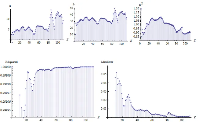
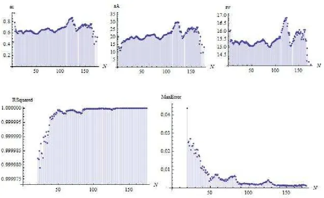
Figure2: The dependence of Weiszäcker model parameters on the number of

protons, the lower figures show the value of standard deviation RSquared and

(16)

Note the similarity in the behavior of parameters of three models: the

parameters reach extreme values at the same or similar values of Z - Table 3. These

results indicate the presence of nuclear structure, but the point of extremes do not

coincide with the magic numbers of protons - 2, 8, 20, 28, 50, 82, as defined in the

standard nuclear shell model [3-6]. A similar result was obtained in [11], in which

the local parameters 5D model depending on the number of neutrons have been

calculated. As it turned out, the number of neutrons corresponding to the extreme

values of the parameters of the model 5D, close to the magic numbers, but nowhere

with them do not match.

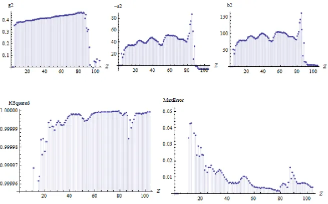
Figure 3: The dependence of the parameters of the 5D model on the number

(17)

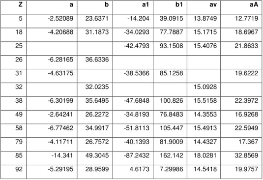
In this regard, we note in Table 3 and Fig. 2-4 three points that fall on the

elements Z = 31,32,85 - Ga (Gallium), Ge (germanium), At (astatine). Gallium and

germanium were predicted by Mendeleev in 1870 and discovered in 1875 and

1885, respectively. Astatine predicted by Mendeleev was artificially synthesized

only in 1940. Note three extreme coinciding with the Z = 26, 79, 92 - Fe (iron), Au

(gold) and U (uranium). There is no doubt that the iron is clearly identified in

nature and has long been used in human practice. The role of gold and uranium in

human history cannot be overestimated. It is also interesting that only in the 5D

model, the binding energy of one of the extremes have the element with proton

number Z = 26 - iron.

Figure 4: The dependence of the parameters of the information model on the

(18)

Table 3: Extreme values of the model parameters

Z a b a1 b1 av aA

5 -2.52089 23.6371 -14.204 39.0915 13.8749 12.7719

18 -4.20688 31.1873 -34.0293 77.7887 15.1715 18.6967

25 -42.4793 93.1508 15.4076 21.8633

26 -6.28165 36.6336

31 -4.63175 -38.5366 85.1258 19.6222

32 32.0235 15.0928

38 -6.30199 35.6495 -47.6848 100.826 15.5158 22.3972

49 -2.64241 26.2272 -34.8193 76.8483 14.3553 16.9268

58 -6.77462 34.9917 -51.8113 105.447 15.4913 22.5949

79 -4.11711 26.7572 -40.1393 81.9009 14.4327 17.367

85 -14.341 49.3045 -87.2432 162.142 18.0281 32.8569

92 -5.29195 28.9599 4.6173 7.29986 14.5418 19.9757

We can assume that there is a version of the periodic table, in which periods

are associated with the trend shown in Fig. 2-4 and in Table 2. These results

suggest that the periodic properties of the nuclei of atomic elements depend on the

number of protons (charge), in line with the modern formulation of the periodic law

[14]. It has been previously established [11] that the periodic properties of nuclei

depend on the number of neutrons, which is reflected in the original formulation of

Mendeleev's periodic law. The Appendix gives the texts of programs to calculate

(19)

Figure 5: The dependence of Weiszäcker model parameters on the number of

neutrons, the lower figures show the value of standard deviation and maximum

absolute prediction error of the binding energy.

Model (24) used in this case without change and 5D model takes the form

) ) ( 1 )( 1 (

/ /

2 2

2

gZ k Z

A bZ a

A Eb

+ + +

= ₍₂₇₎

Since the 5D model is rigid, it uses a numerical coefficient k, which provides

the convergence of solutions depending on the number of neutrons in the form

(20)

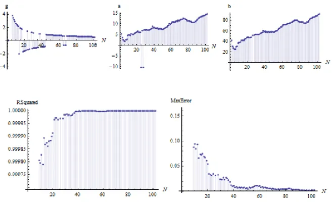
Figure 6: The dependence of the parameters of the 5D model on the number

of neutrons.

The data presented in Fig. 5 that the Weiszäcker model parameters depend

on the number of neutrons, and these dependencies are not monotonic, which

indicates the presence of nuclear structure. Thus, we have shown that the binding

energy of all known nuclides can be described approximately with the same

accuracy by any of three models (24)-(26). This means that the nucleus can be

regarded as a charged liquid drop (Weiszäcker model), and as a set of shielded

"clean" protons in the five-dimensional space [10-11], and as a statistical

(information) system [12].

Note that the droplet model of the nucleus had a large development in the

30-50s of last century. On the other hand, 5D model is theoretically justified by Kaluza

[15], Einstein [16-19], Pauli and Einstein [20], Rumer [21], Dzhunushaliev [22],

(21)

great potential in terms of its expansion, taking into account the spin angular

momentum and other quantum numbers, as well as quantum chaos [6-7, 23-24].

The author expresses his gratitude to Professor VD Dzhunushaliev and Professor EV Lutsenko for

useful discussions.

References

1. МенделеевД. И., Периодический закон. Основныестатьи. — М.: Изд-воАН СССР, 1958, с. 111.

2. Iwanenko, D.D. The neutron hypothesis// Nature, 129, 1932, 798.

3. ИваненкоД.Д., Периодическаясистемахимическихэлементовиатомноеядро //

Д.И.Менделеев. Жизньитруды, АНСССР, М., 1957, с.66-100. 4. ГейзенбергВ. Замечанияктеорииатомногоядра// УФН (1), 1936.

5. Maria Goeppert-Mayer. On Closed Shells in Nuclei/ DOE Technical Report, Phys. Rev. Vol. 74; 1948. II DOE Technical Report, Phys. Rev. Vol. 75; 1949

6. P. Leboeuf. Regularity and chaos in the nuclear masses/ Lect. Notes Phys. 652, Springer, Berlin Heidelberg 2005, p.245, J. M. Arias and M. Lozano (Eds.).

7. Jorge G. Hirsch, Alejandro Frank, Jose Barea, Piet Van Isacker, Victor Velazquez. Bounds on the presence of quantum chaos in nuclear masses//Eur. Phys. J. A 25S1 (2005) 75-78 8. Wolfram Mathematica 8// http://www.wolfram.com/mathematica/

9. ТруневА.П. Фундаментальные взаимодействияв теорииКалуцы-Клейна// Научный

журнал КубГАУ. – Краснодар: КубГАУ, 2011. – №07(71). С. 502 – 527. – Режим

доступа: http://ej.kubagro.ru/2011/07/pdf/39.pdf

10.A. P. Trunev. The structure of atomic nuclei in Kaluza-Klein theory // Политематический

сетевойэлектронныйнаучныйжурналКубанскогогосударственногоаграрного университета (НаучныйжурналКубГАУ) [Электронныйресурс]. – Краснодар:

КубГАУ, 2012. – №02(76). С. 862 – 881. – Режимдоступа: http://ej.kubagro.ru/2012/02/pdf/70.pdf

11.Трунев А.П. Ядерные оболочки и периодический закон Д.И. Менделеева//

Политематический сетевой электронный научный журнал Кубанского государственногоаграрногоуниверситета (НаучныйжурналКубГАУ) [Электронный

ресурс]. – Краснодар: КубГАУ, 2012. – №05(79). С. 414 – 439. – Режим доступа: http://ej.kubagro.ru/2012/05/pdf/29.pdf

12.Луценко Е.В. Количественная оценка уровня системности на основе меры

информации К. Шеннона (конструирование коэффициента эмерджентности

Шеннона) / Е.В. Луценко // Политематический сетевой электронный научный

журнал Кубанского государственного аграрного университета (Научный журнал

КубГАУ) [Электронный ресурс]. – Краснодар: КубГАУ, 2012. – №05(79). С. 249 – 304. – Режимдоступа: http://ej.kubagro.ru/2012/05/pdf/18.pdf

13.Marselo Alonso, Edward J. Finn. Fundamental University Physics. III Quantum and Statistical Physics. – Addison-Wesley Publishing Company, 1975.

(22)

15.Kaluza, Theodor. Zum Unitätsproblem in der Physik. Sitzungsber. Preuss. Akad. Wiss.

Berlin. (Math. Phys.)1921: 966–972.

16.Альберт Эйнштейн. К теории связи гравитации и электричества Калуцы II. (см.

АльбертЭйнштейн. Собраниенаучныхтрудов. Т. 2. – М., Наука, 1966)

17.Альберт Эйнштейн, В. Баргман, П. Бергман. О пятимерном представлении

гравитациииэлектричества (см. АльбертЭйнштейн. Собраниенаучных трудов. Т. 2. – М., Наука, 1966 статья 121).

18.АльбертЭйнштейн. Собраниенаучныхтрудов. Т. 2. – М., Наука, 1966, статья 122. 19.A. Einstein, P. Bergmann. Generalization of Kaluza’s Theory of Electricity// Ann. Math.,

ser. 2, 1938, 39, 683-701 (см. АльбертЭйнштейн. Собраниенаучныхтрудов. Т. 2. –

М., Наука, 1966)

20.Einstein A., Pau1i W.— Ann of Phys., 1943, v. 44, p. 131. (см. Альберт Эйнштейн.

Собраниенаучныхтрудов. Т. 2. – М., Наука, 1966, статья 123).

21.Ю. Б. Румер. Исследованияпо 5-оптике. – М., Гостехиздат,1956. 152 с.

22.V. Dzhunushaliev. Wormhole solutions in 5D Kaluza-Klein theory as string-like objects//

arXiv:gr-qc/0405017v1

23.Vladimir Zelevinsky. Quantum Chaos and nuclear structure// Physica E, 9, 450-455, 2001.

24.Alexander P. Trunev. Binding energy bifurcation and chaos in atomic nuclei//

Политематический сетевой электронный научный журнал Кубанского государственного аграрного университета (Научный журнал КубГАУ) [Электронный ресурс]. – Краснодар: КубГАУ, 2012. – №05(79). С. 403 – 413. –

Режимдоступа: http://ej.kubagro.ru/2012/05/pdf/28.pdf, 0,688 у.п.л.

Appendix

Source code for calculating the Weiszäcker model parameters in Table 2:

Do[ model = av - 17.23*(Z + x)^(-1/3) + ac*(Z*Z)*(Z + x)^(-4/3) + aA*((x - Z)^2)*(Z + x)^(-2);

Eb = Table[IsotopeData[#, prop], {prop, {"NeutronNumber", "BindingEnergy"}}] & /@ IsotopeData[Z];

nlm = FindFit[Eb, model, {{ av, 15.5}, {ac, -.628528}, {aA, -22.03}}, x]; Print[Z, nlm], {Z, 1, 118}]

Source code for the comparison of three models - Fig. 1:

Z = 78; k = 0.000049;

Eb = Table[IsotopeData[#, prop], {prop, {"NeutronNumber", "BindingEnergy"}}] & /@ IsotopeData[Z];

nlm = NonlinearModelFit[Eb, a + b*(x*x/(Z*1. + x))*((x^2 + 1)*(1 + k*(g*x)^2))^(-.5) , {a, b, g}, x];

nlm1 = NonlinearModelFit[Eb, av - 17.23*(Z + x)^(-1/3) - ac*(Z*Z)*(Z + x)^(-4/3) - aA*((x - Z)^2)*(Z + x)^(-2) , {av, ac, aA}, x];

nlm2 = NonlinearModelFit[Eb, a2 + b2*(x/(Z*1. + x))*(-Log[x/(Z*1. + x)] + g2) , {a2, b2, g2}, x];

Show[ListPlot[Eb], Plot[{nlm[x], nlm1[x], nlm2[x]}, {x, 1., 180.}, PlotStyle -> {Red, Green, Blue}], Frame -> True,

FrameLabel -> {N, "Eb/A, MeV"}]

Source code for calculating the Weiszäcker model parameters depending on

the number of protons (Fig. 2):

par = {0.}; para = {0.}; parc = {0.}; RSq = {1.}; MaxEr = {0.};

Do[ Eb = DeleteCases[Table[IsotopeData[#,prop], {prop, {"NeutronNumber", "BindingEnergy"}}] & /@

(23)

nlm = NonlinearModelFit[Eb, av - 17.23*(Z + x)^(-1/3) - ac*(Z*Z)*(Z + x)^(-4/3) - aA*((x - Z)^2)*(Z + x)^(-2) , {av, ac, aA}, x];

RSq = {RSq, nlm["RSquared"]} // Flatten;

MaxEr = {MaxEr, Last[Sort[nlm["MeanPredictionErrors"]]]} // Flatten;

para = {para, av /. nlm["BestFitParameters"]} // Flatten;

parc = {parc, ac /. nlm["BestFitParameters"]} // Flatten;

par = {par, aA /. nlm["BestFitParameters"]} // Flatten, {Z, 2, 112}]

ListPlot[par, Filling -> Axis, AxesLabel -> {Z, aA},

ImageSize -> {200, 200}] ListPlot[para, Filling -> Axis,

AxesLabel -> {Z, av}, ImageSize -> {200, 200}] ListPlot[parc,

Filling -> Axis, AxesLabel -> {Z, ac}, ImageSize -> {200, 200}]

ListPlot[RSq, Filling -> Axis, AxesLabel -> {Z, "RSquared"},

ImageSize -> {300, 300}, DataRange -> Automatic] ListPlot[MaxEr,

Filling -> Axis, AxesLabel -> {Z, "MaxError"},

ImageSize -> {300, 300}, DataRange -> Automatic]

Source code for calculating the Weiszäcker model parameters depending on

the number of neutrons (Fig. 5):

par = {.0}; para = {.0}; parc = {.0};

Do[model = av - 17.23*(nn + x)^(-1/3) - ac*(x*x)*(nn + x)^(-4/3) - aA*((x - nn)^2)*(x + nn)^(-2) ;

Eb = Drop[

Cases[DeleteCases[

Table[{a - z, z, IsotopeData[{z, a}, "BindingEnergy"]}, {z, 1, 118}, {a,

IsotopeData[#, "MassNumber"] & /@ IsotopeData[z]}], {_, Missing["Unknown"]}] // Flatten[#, 1] &, {nn, _, _}], None, {1}];

nlm = FindFit[Eb, model, {{ av, 15.5}, {ac, 0.628528}, {aA, 22.03}}, x]; para = {para, av /. nlm} // Flatten;

parc = {parc, ac /. nlm} // Flatten;

par = {par, aA /. nlm} // Flatten, {nn, 2, 175}] ListPlot[par, Filling -> Axis, AxesLabel -> {N, aA}] ListPlot[para, Filling -> Axis, AxesLabel -> {N, av}] ListPlot[parc, Filling -> Axis, AxesLabel -> {N, ac}]

Source code for calculating the dependence of 5D model parameters on the

number of protons (Fig. 3):

par = {0.}; para = {0.}; parc = {0.}; RSq = {1.}; MaxEr = {0.};

Do[ Eb = DeleteCases[Table[IsotopeData[#, prop], {prop, {"NeutronNumber", "BindingEnergy"}}] & /@

IsotopeData[Z], {_, Missing["Unknown"]}];

nlm = NonlinearModelFit[Eb, a + b*(x*x/(Z*1. + x))*((x^2 +1)*(1 + (0.9592/Z^2.209)*(g*x)^2))^(-.5), {a, b, g}, x];

para = {para, -a /. nlm["BestFitParameters"]} // Flatten;

(24)

parc = {parc, b /. nlm["BestFitParameters"]} // Flatten;

par = {par, g^2 /. nlm["BestFitParameters"]} // Flatten, {Z, 2, 110}]

ListPlot[par, Filling -> Axis, AxesLabel -> {Z, "g"}, ImageSize -> {200, 200}, PlotRange -> {0.8, 1.2}] ListPlot[para,

Filling -> Axis, AxesLabel -> {Z, "a"}, ImageSize -> {200, 200}] ListPlot[parc, Filling -> Axis,

AxesLabel -> {Z, "b"}, ImageSize -> {200, 200}]

ListPlot[RSq, Filling -> Axis, AxesLabel -> {Z, "RSquared"}, ImageSize -> {200, 200}, DataRange -> Automatic] ListPlot[MaxEr,

Filling -> Axis, AxesLabel -> {Z, "MaxError"},

ImageSize -> {200, 200}, DataRange -> Automatic]

Source code for calculating the dependence of 5D model parameters on the

number of neutrons (Fig. 6):

par = {0.};para = {0.};parc = {0.};RSq = {0.};MaxEr = {0.};

Do[ Eb = Drop[ Cases[DeleteCases[

Table[{a - z, z, IsotopeData[{z, a}, "BindingEnergy"]}, {z, 1,118}, {a, IsotopeData[#, "MassNumber"] & /@ IsotopeData[z]}],

{_,Missing["Unknown"]}] // Flatten[#, 1] &, {nn, _, _}], None, {1}];

nlm = NonlinearModelFit[Eb, a + b*(x* x/(nn*1. + x))*((x^2 + 1)*(1 + (0.0025 - 0.0003*Log[nn])*(g*x)^2))^(-.5), {a, b, g}, x];

para = {para, -a /. nlm["BestFitParameters"]} // Flatten;

RSq = {RSq, nlm["RSquared"]} // Flatten;

parc = {parc, b /. nlm["BestFitParameters"]} // Flatten;

par = {par, g /. nlm["BestFitParameters"]} // Flatten, {nn, 2, 102}]

ListPlot[par, Filling -> Axis, AxesLabel -> {N, "g"},

ImageSize -> {200, 200}] ListPlot[para, Filling -> Axis,

AxesLabel -> {N, "a"}, ImageSize -> {200, 200}] ListPlot[parc,

Filling -> Axis, AxesLabel -> {N, "b"}, ImageSize -> {200, 200}]

ListPlot[RSq, Filling -> Axis, AxesLabel -> {N, "RSquared"},

ImageSize -> {200, 200}, DataRange -> Automatic] ListPlot[MaxEr,

Filling -> Axis, AxesLabel -> {N, "MaxError"},