Abstract
The paper concerns topology and geometry optimization of stati-cally determinate beams with an arbitrary number of pin supports. The beams are simultaneously exposed to uniform dead load and arbitrarily distributed live load and optimized for the absolute max-imum bending moment. First, all the beams with fixed topology are subjected to geometrical optimization by genetic algorithm. Strict mathematical formulas for calculation of optimal geometrical pa-rameters are found for all topologies and any ratio of dead to live load. Then beams with the same minimal values of the objective function and different topologies are classified into groups called topological classes. The detailed characteristics of these classes are described.
Keywords
Statically determinate beams, geometry and topology optimiza-tion, genetic algorithm, stationary load, most unfavorable load.
Geometry and Topology Optimization of Statically Determinate
Beams under Fixed and Most Unfavorably Distributed Load
NOMENCLATURE
n i
b , bi assignment of lengths
l
Bj to left or right side of supports, i1, 2,...,nE
c , cH number of external and internal cantilevers
B j
c number of j-th cantilevers from the top of the beam interaction scheme, 1, 2, 1
j n
g beam chromosome
h coordinates of hinges
l,lE,lH,L lengths of optimal beam segments and length of beam, see Fig. 1
B j
l distance from intersection of optimal moment diagram (with maximum value n i
M at the
bottom) with beam axis to the nearest support, j1, 2,n1, see Fig. 1 and Fig. 2 i
M , n
i
M optimal moment value of topology ti and class Tin
Agata Kozikowska *
Bialystok University of Technology, Fac-ulty of Architecture, Bialystok, Poland
* corresponding author email:
http://dx.doi.org/10.1590/1679-78252306
NOMENCLATURE (continuation)
n number of supports n
p ,p2:n number of topological classes in set n
T
andT
2:nq dimensionless intensity of uniformly distributed gravity dead load for constant sum of gravity dead load and maximum gravity live load intensities, equal to one, 0 q 1 1q maximum dimensionless intensity of arbitrarily distributed live load for constant sum
of both load intensities, equal to one R equivalence relation of beam topologies s coordinates of supports
i
t beam topology
i
t topological code of support i, i1, 2,...,n n
T ,T2:n set of all topologies with
n
supports and with two ton
supports ni
T ,Ti2:n topological class with
n
supports and with two ton
supportsx
axial coordinatei
y dimensionless length of cantilever, i1, 2,...,n
i
z dimensionless length of span, i1, 2,...,n
( )
n, ( ) ni quantities in set Tn and class n i
T
1 INTRODUCTION
Structural optimization, which includes sizing, geometry, and topology optimization, has been a very common topic of research. Topology optimization is a relatively new but fast growing field of this research (Kirsch, 1989; Rozvany et al., 1995; Eschenauer and Olhoff, 2001; Fancello and Pereira, 2003; Marczak, 2008; Rozvany, 2009; Lopes et al., 2015). In recent years, structural topology optimization has received a boost due to the recognition that topological parameters can lead to a significant improvement in the quality of structures. Thanks to the widespread availability of high-speed com-puters and the development of powerful computational methods for the structural analysis, scientists can return to problems considered to be investigated and can make new interesting discoveries. The topological optimization of statically determinate beams is such an insufficiently explored problem.
of different distributions (Rychter and Kozikowska, 2009; Kozikowska, 2011) and under the most unfavorably distributed load (Kozikowska, 2014).
Beam loads are generally a combination of dead and live loads. Dead load is essentially constant and can be treated as uniformly distributed, especially for beams with constant cross-sections. Live load can vary during the life of the structure. In the paper both loads occur simultaneously. It is assumed that live load is characterized by a relatively slow increase of the magnitude and it is regarded as static (without dynamic effects).
Beams are usually subjected to transverse loadings, which result in internal shear forces and bending moments. In the article we consider beams which are relatively long in comparison with their thickness and depth. Bending stresses have the greatest effect on the behavior of such beams and they can be designed mainly against bending moment resistance. Therefore the structural measure of beams is defined in the paper as the absolute maximum bending moment, like in Wang (2006). For beams with uniform cross-sections this measure corresponds to the design for minimum weight. The most adverse distributions of the live load for all cross-sections of a beam can be obtained with the help of influence lines for bending moment.
Due to the complexity of the geometric search space of statically determinate beam with any number of supports, geometry optimization of beams is performed using a genetic algorithm. This method of probabilistic optimization have been applied to a great variety of structural optimization problems (Wang and Chen, 1996; Castro and Partridge, 2006; Rychter and Kozikowska, 2009).
Results of topology optimization, occurring in the literature, usually depend on an initial layout, which is adopted arbitrarily. The final solutions are then obtained by exploring only some parts of the full search space and they are not necessarily the best topological layouts. In the paper the space of all possible beam topologies is known, exhaustive search in this space is carried out and global optima are determined. Moreover, the paper presents not only globally optimal beam topologies, but classifies all topologies into equivalence classes with equal minimum values of the absolute maximum moment. Typical features of these classes are discussed.
2 BEAM TOPOLOGY AND GEOMETRY
The subject of the paper is the space of all statically determinate beams with different topologies, with two or more pin supports. The construction of all possible topologies of beams with
n
pin supports, solved by Rychter (Rychter and Kozikowska, 2009), starts with the topology, where alln
ends of all bars are supported. Then each support can be shifted from the end of a bar (first and last support), or the common hinged end of two adjacent bars (intermediate supports), into the interior of a bar, but not to a distant bar. The topology ti of an
n
-support statically determinate beam is represented byn
topological codes of supports ti:{0, 2} for 1,
{0,1, 2} for {2, , 1},
{0,1} for , i
i
t i n
i n
(1)
The geometry of a beam is described by two sets of geometric parameters: zi and yi. The param-eters zi are dimensionless lengths of spans between neighbour supports:
0zi 1, i{1, 2,...,n1} (2)
The parameters yi represent dimensionless lengths of external and internal cantilevers:
1 1
0 if 0, {1, 2,..., }
0 1 if 0, {1, 2,..., }
1 if 1 2, {2,..., 2}
i i
i i
i i i i
y t i n
y t i n
y y t t i n
(3)
When support i is at the end of the beam or at the hinge, no cantilever is created, and the parameter
i
y equals zero – the first row in Eq. (3). Otherwise, the parameter yi takes real value from the interval (0,1) – the second row in Eq. (3). The third row in Eq. (3) prevents the cantilevers from overlapping. For the external cantilevers the parameters y1,yn are dimensionless lengths. For the internal cantilevers the parameters y2,...,yn1 are ratios of lengths of cantilevers to the lengths of spans in which the cantilevers reside.
The total length of a beam is the sum of the lengths of all spans and the lengths of the external cantilevers. All beams have the same length, normalized to unity:
1 1 2 ... n 1 n 1
L y z z z y (4)
A more detailed description of the topological and geometrical parameters is given in Rychter and Kozikowska (2009).
3 GEOMETRY OPTIMIZATION OF A BEAM WITH A FIXED TOPOLOGY
3.1 Problem Formulation
the ones that result in the maximum values of bending moment. The issues discussed in the article do not depend on the absolute values of the dead and live load intensities, but only on their ratio. Therefore we normalize both intensities so that their sum is constant, equal to one. The intensity of dead load is equal to q and the maximum intensity of live load is equal to 1q. Each intensity can take values from 0 to 1.
Beams under arbitrarily distributed transverse live loads, considered in the author's article (Kozikowska, 2014), had two most unfavorable load cases for the maximum bending moment. Each case included uniformly distributed load of maximum intensity on alternate spans. If we take dead and live load into account, we also have two load cases. One of the cases comprises uniform load of intensity 1 (sum of both loads) on odd spans and uniform dead load of intensity q on even spans. The second case also includes uniform loads: q on odd spans and sum of loads equal to 1 on even spans.
We assume that each beam is of unit length with a fixed topology ti. The geometry optimization problem is defined as follows:
[0,1]
Minimize max |
( ,
i j, ) |
x
M z y x
(5)1 1 2 1
0 1 1, 2, , 1
Subject to 0 1 for 0 1, 2, , 1 i
j j
n n
z i n
y t j n
y z z z y
(6)
where
[0,1]
max | ( ,i j, ) |
x M z y x denotes the maximum of the absolute bending moment (objective function) for both load cases, zi are span lengths given by Eq. (2), yj are nonzero lengths of cantilevers, which are created by shifts of supports of nonzero topological codes tj from ends of bars, given by Eq. (3), and
x
is the axial coordinate.This geometry optimization has been carried out by a modified version of the genetic algorithm (Rychter and Kozikowska, 2009), written by the author in C/C++ programming language.
3.2 Genetic Algorithm
The genetic algorithm for the optimization of the geometry of statically determinate beams follows the general scheme of genetic algorithms (Goldberg, 1989). Populations of chromosomes are evolved over several generations, subject to random mutation, random crossover (recombination), and selec-tion pressure.
The chromosome g representing a geometry of a
n
-support statically determinate beam with a fixed topology ti is a string ofn
1
real genes zi and (cE cH) real nonzero genes yj:1 1
[ ,
z
,
z
n,...,
y
j,...]
g
(7)The creation of an initial population involves the assignment of random real values from the interval (0,1) to all genes, and then the adjustment of the genes to the conditions contained in the third row of Eq. (3) and in Eq. (4).
The designed chromosomes allow for easy random mutation and crossover, without producing incorrect beams. After these operations, the chromosomes only have to be adjusted to the conditions given in the third row of Eq. (3) and in Eq. (4). The most efficient versions of mutation, crossover and selection have been determined through extensive simulations.
Gaussian mutation, in which a Gaussian distributed random value is added to the value of the chosen gene, has turned out to be the best mutation method.
The performance of algorithm with single-point crossover was the same as with multi-point cross-over. Yet the former is simpler and faster than the latter. Therefore, single-point recombination has been used where two parent chromosomes are cut in one random point, and both chromosome parts are swapped to produce two children.
Three selection strategies have been studied: proportional roulette-wheel, proportional determin-istic, and ranking tournament. The tournament selection involves running several tournaments (groups of chromosomes) chosen at random from population members. The winners of all tournaments go into the next population. Moreover, in the applied tournament strategy, the best beam must fall into at least one tournament group and so will always survive selection. Numerical simulations have shown the superiority of this tournament selection with binary tournaments over proportional selec-tion methods.
The minimal value of the absolute maximum bending moment Mi has been found for each to-pology ti as a result of the optimization by this genetic algorithm.
3.3 Optimization Results
A beam with optimal geometry for the fixed topology is presented in Fig. 1. The beam is shown with two unique bending moment diagrams, drawn with a solid line or a dashed line, for both the most unfavorable load cases. The optimal envelope of the two moment diagrams has the same local extreme moment values equal to Mi. These values are present over the supports which were moved away from ends of bars and at the bottom at mid spans or close to them. The envelope has zero values exclusively in hinges and at both ends of the beam and is equivalent to only one topology, unlike in the case of dead load alone (Kozikowska, 2011).
We are interested in analytical expressions for optimal geometrical parameters for any topology, under stationary load and the most unfavorably distributed load. In order to determine the values of the parameters l, lE, lH, and lB j for 1, 2,j ,n1 (see Fig. 1) we solve the system of equations:
1
1
(
1)
n
E E H H Bj Bj
j
n
l
c l
c l
c l
L
(8)1
0
2llE (9)
2 2
4
H4( )
H0
l
ll
l
(10)1 1
(llB )lB q l( lH)lH 0 (11)
2( 1) ( 1)
1
( ) ( ) ( ) 0
4
B j Bj Bj H B j H H
ll ll l q ll l l l l (12)
where lE and lH denote the lengths of nonzero external and internal cantilevers, respectively,
l
is the length of each segment with at least one of the two optimal moment diagrams at the bottom, with the maximum value of this moment equal to Mi and zero values of this moment at both ends of the segment, lB j for j1, 2,n1 is the distance from intersection of optimal moment diagram (with maximum value Mi at the bottom) with beam axis to the nearest support, moreover there is no hinge in zero moment point. The lengthsl
Bj neighbour on the external and internal cantilevers. The indicesj
inl
Bj are consecutive numbers of these neighbouring cantilevers, counted from the top of the inter-action scheme of the beam (see Fig. 2). The neighbouring cantilevers, which form consecutive levels (steps) in the interaction diagram, create sequences. The number of terms (cantilevers) in such a se-quence is the length of the cantilever sese-quence. The pseudo code for an algorithm to assign the lengthsBj
l
to supports on the basis of the beam topology is given in appendix A. The algorithm returns a vectori
b of
n
integer elements bk. The element bk is equal toj
if the lengthl
Bj is on the right side of the support k , is equal to
j
if the lengthl
Bj is on the left side of the support k , and is equal to zero if there is no lengthl
Bj next to support k (the support k is at the end of the beam or under a hinge). For example, bi [1, 2, 3, 2, 1, 0, , 0,1, 1] for the beam from Fig. 2.Figure 2:Locations of lengths lB j depending on consecutive numbers of cantilevers
Equation (8) describes the length of the beam as the sum of individual segment lengths. The parameters cE, cH, cB j for j1, 2,n1 are the numbers of the segments lE, lH,
for 1, 2, 1 B j
l j n , respectively. The lengths of a cantilever and a simply supported beam with the same values of the absolute maximum moment under uniformly distributed dead and live load are compared in Eq. (9). The maximum bending moment value of a simply supported beam of the length
2H
l l equals twice this moment value of a simply supported beam of the length
l
in accordance with Eq. (10). Eq. (11) is explained graphically in Fig. 3. The equation was established by comparing the moment value at the support calculated on the basis of the moment diagram on the left of the support with this moment value calculated according to the moment diagram on the right. Eq. (12) was found from the moment diagram, drawn with a solid line in Fig. 4.Figure 3:Graphic explanation of Eq. (11).
Figure 4:Graphic explanation of Eq. (12).
The solution to the system of equations (8)–(12) is given by:
L l
d
(13)
2 E
L l
d
2 1
2 H
L l
d
(15)
1
for 1, , 12 Bj j
L
l B j n
d
(16)
where
1
1
1
1
1
( 2 1)
1
1
2
2
2
n
E H j Bj
j
d
n
c
c
B
c
1
1
B
q
( 1)
( 1)
2 1
1 2 1 2 for 2, , -1
1
j j
j
B q B j n
B
The values of the parameters cE and cH can be determined from the beam topology ti. The value of the parameter cE is equal to the number of nonzero elements in the first and last position of the code ti. The value of the parameter cH is the number of nonzero elements in positions 2 through n1 of the code ti. An algorithm to calculate the values of parameters
c
Bjfor
j
1,2,
n
1
on the basis of the vector bi (assigning the lengthsl
Bj to supports) is given by a pseudo code in appendix B. The value of the absolute maximum bending moment Mi can be calculated as the moment in the centre of a simply supported beam of the lengthl
under uniform load equal to the sum of both loads (intensity equal to one):2
8
iM
l
(17)Algorithms to calculate the coordinates of supports and hinges (on the basis of the beam topology, the vector bi, and the lengths l, lE, lH, and lB j for 1, 2,j ,n1) are given by a pseudo code in appendix C.
3.4 Dependence of Optimal Geometrical Parameters on Dimensionless Dead Load Intensity q
The formulas (13)–(16) enable us to calculate the optimal lengths of the segments l, lE, lH,
for 1, 2, 1 B j
l j n for any number of supports, for any topology, and for any value of the dimen-sionless dead load intensity 0 q 1. For the extreme values of q, equal to 0 or 1, we receive special cases with specific values of lB j.
B j
l
is on the same side of the support as the segment lH (see Fig. 5a for the beam with the topology [2,2,1,1]).For q1 (only fixed load) regardless of the beam topology, both load cases come down to one case with dead load on the entire beam, and all segments lB j for 1,j n1 have the same length equal to the length lH (see Fig. 5c for the beam with the topology [2,2,1,1]).
For 0 q 1 (fixed load and most unfavorably distributed load acting simultaneously) regardless of the beam topology, all optimal segment lengths have different values. The segments lB j are shorter than lH, while l, lE are longer than lH. The value of the parameter lB1 is more than zero, but for small values of q (less than about 0.2) the lengths
l
B jfor 2,
j
n
1
are less than zero.The lengths of the optimal beam segments can also be calculated in case of live load alone using the formulas presented in Kozikowska (2014) and in case of dead load alone using the formulas given in Kozikowska (2011). The sets of optimal geometrical parameters which have been used in the pre-vious author's articles consist of a smaller number of parameters than the set used in this paper. Therefore, the sets used in Kozikowska (2014, 2011) cannot be applied to describe the optimal geom-etry of the statically determinate beams for 0 q 1.
Figure 5:The beam with optimal geometry for the topology [2,2,1,1] and for different values of the
The dependence of optimal segment lengths on values of q is illustrated in Fig. 6 with regard to the beam from Fig. 5 (with the topology [2,2,1,1]). The values of the parameters l, lE, lH are more than zero for all values of 0 q 1, and the values l, lE, lH are the biggest for q0. For q0, the value of the parameter lB1 is equal to zero, but lB2 is less than zero. Next, the values of the parameters l, lE, lH decrease with increasing q, lB1 and lB2 increase with increasing q, and lB1 and lB2 reach the value lH for q1. For q greater than zero but less than a value of about 0.2, the value of the parameter lB2 is less than 0. The dependence of the parameters l, lE, lH,
for
1, 2,
1
B jl
j
n
on q is the same for beams with any number of supports and any topology.Figure 6:Lengths l, lE, lH, lB1, and lB2 of the beam from Fig. 5 (with the topology [2,2,1,1])
for different values of the dimensionless dead load intensity q .
4 TOPOLOGY OPTIMIZATION OF BEAMS WITH A FIXED NUMBER OF SUPPORTS FOR 0 <
q
< 1Topology optimization of beams with a fixed number of supports for q0 (live load alone) is pre-sented in Kozikowska (2014) and for q1 (dead load alone) in Kozikowska (2011).
4.1 Equivalence Relation of Beam Topologies
T is the set of n-support beam topologies: Tn or T2:n. Any two topologies
t
i andt
j of the set T are equivalent with respect to the relation R if the minimal values of the absolute maximum momentsi
M and
M
j of these topologies are equal:if
i
R jM
i
M
jt
t
(18)Based on this relation R, the set Tn can be divided into disjoint equivalence classes of beam topologies called topological classes n
i
T , and the set T2:n into topological classes 2:n i
4.2 Features of Beam Topologies in a Topological Class
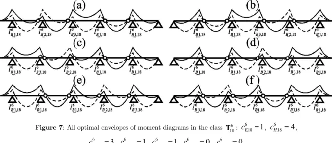
All optimal bending moment diagram pairs from the topological class 6 18
T (the eighteenth class of all
six-support classes ordered by increasing values of moments n i
M ), under a fixed uniformly distributed
load and the most unfavorably piece-wisely distributed load, are shown in Fig. 7.
Figure 7:All optimal envelopes of moment diagrams in the class 6
18
T : c6E,18 1, 6
18 4
H,
c ,
6 1 18 3
B ,
c , 6 2 18 1
B ,
c , 6 3 18 1
B ,
c , 6
4 18 0
B ,
c , 6
5 18 0
B ,
c .
All topologies in the topological class n i
T have the same values of moment n i
M and lengths
l
in, nE,i
l
, nH,i
l
, lB k,in for k1, 2,n1. The lengths n il
, nE,i
l
, nH,i
l
, lB k,in for 1, 2,k n1, given by Eq. (13)–(16), depend on the number of supports, the values of the param1eters n E,i
c
, nH,i
c
, andfor 1, 2, 1 n
B k,i
c k n , and the value of q. Thus for two topologies
t
i andt
j of the set nT under a fixed and the most unfavorably distributed load the equivalent condition from Eq. (18) can be expressed as:
, , , , , ,
if
for
1,
,
1
i
R jc
E i
c
E j
c
H i
c
H j
c
Bk i
c
Bk jk
n
t
t
(19)where
c
E i, ,c
H i, ,c
Bk i,for 1,2,
k
n
1
,c
E j, ,c
H j, ,c
Bk j,for 1,2,
k
n
1
are the numbers of theappropriate segments for the topology
t
i andt
j, respectively.4.3 Comparison of Topological Classes
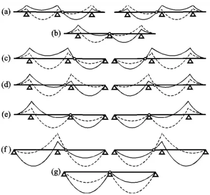
Figure 8: All three-support topological classes with their optimal envelopes of moment diagrams: (a) 3
1
T , (b) 3 2
T , (c) 3 3
T , (d) 3 4
T , (e) 3 5
T , (f) 3 6
T , (g) 3 7
T (q1 2).
Figure 9:All three-support topological classes with their optimal envelopes of moment diagrams:
(a) 3 1
T , (b) 3 2
T , (c) 3 3
T , (d) T43, (e) 3 5
T , (f) 3 6
T , (g) 3 7
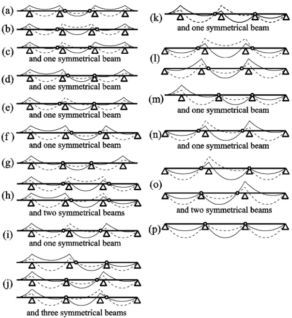
Figure 10:All four-support topological classes with their optimal envelopes of moment diagrams: (a) 4
1
T , (b) T24, (c) 4 3
T , … , (p) T164 (q1 2).
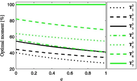
The division of beam topologies into topological classes does not depend on the value of the dead to live load ratio. This ratio only affects the optimal values of the geometrical parameters, which can be calculated from the formulas (13)–(16). The lengths n
E,i
l
, nH,i
l
, ni
l
, and the moment value n iM are
greater for smaller values of the ratio (for smaller values of dimensionless dead load intensity q) for all classes except for the last class whose optimal moment is independent of q. The dependence of values n
i
M on q in three-support classes is shown in Fig. 11. It is observed that the growth of q (smaller share of live load) makes moment values decrease, except for the last class 3
7
Figure 11:Optimal moments in three-support topological classes for different values of the dimensionless dead load intensity q .
The division of all topologies into topological classes depends on the number of cantilevers and their locations in the interaction diagram of the beam (see Fig.2). The topological classes are the better, the more cantilevers their beams have (the more external cantilevers for the same total number of cantilevers) and the shorter the lengths of the cantilever sequences are in the interaction schemes. In other words, better classes have larger values of the parameters n
E,i
c
and n H,ic
(have larger values ofthe parameters n E,i
c
than the parameters n H,ic
for the same sum of n E,ic
and n H,ic
), and have more zero parameters nBj,i
c . The values of the parameters
c
nE,i, n H,ic
, and cBj,in for 1,j n1 for the three-supportclasses (from Fig. 8 and Fig. 9) and for the four-support classes (from Fig. 10) are given in Table 1 and Table 2, respectively. The best topological class with an odd number of supports have n1 topologies, each with a single one-hinged span (see Fig. 8a and Fig. 9a). The best single topology in the first class with an even number of supports does not have any one-hinged spans (see Fig. 10a).
3
i
T
31
T 3
2
T
T
33 34
T
T
53T
63T
733
E,i
c 2 2 1 1 1 0 0
3
H,i
c 1 0 1 1 0 1 0
3 1,i B
c 2 2 2 1 1 1 0
3 2,i B
c 1 0 0 1 0 0 0
Table 1: Values of the parameters 3
E,i c , 3
H,i c , 3
for 1, 2 B j,i
4
i
T
41
T T24
T
34 44
T
T
54T
64T
74T
84T
94T
104 4 11T T124
T
134 414
T
T
154T
1644
E,i
c 2 2 2 2 2 1 2 1 1 1 1 0 1 0 0 0
4
H,i
c 2 2 2 1 1 2 0 2 2 1 1 2 0 2 1 0
4 1,i B
c 4 2 2 3 2 3 2 2 1 2 1 2 1 1 1 0
4 2,i B
c 0 2 1 0 1 0 0 1 1 0 1 0 0 1 0 0
4 3,i B
c 0 0 1 0 0 0 0 0 1 0 0 0 0 0 0 0
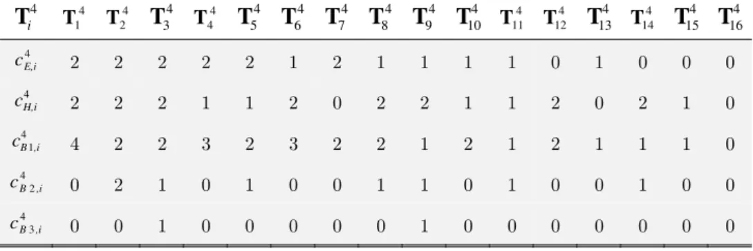
Table 2: Values of the parameters 4
E,i c , 4
H,i
c and 4
for 1, 2,3 B j,i
c j in four-support topological classes.
The set of all
n
-support topological classes is described by the set of all possible (n 1)-element sequences (cE,in ,cH in,,cB j,in for j1, 2,n1) wherec
nE,i
{0,1, 2}
,{0,1,
,
2}
n H,i
c
n
, and values of theparameters n for 1, 2, 1 B j,i
c j n meet the following conditions:
1, 2, , 1
, 0n B j i
j n c
(20)
1, ,
n n
B i E i
c c (21)
1, 2, , 2
, 1,n n
B j i B j i
j n c c
(22)
,2
,2
1,is even
n n n
E i H i B i
c
c
n
c
(23)1
, , ,
1
n
n n n
Bj i E i H i j
c
c
c
(24)The numbers of
j
-th cantilevers from the top of the interaction scheme n Bj,ic are nonnegative (see Eq. (20)). External cantilevers are always at the top of the interaction diagram (they are always the first from the top of the interaction scheme) in accordance with Eq. (21). The number of
j
-th canti-levers from the top of the interaction diagram must be equal to or larger than the number of (j1) -th cantilevers because (j1)-th cantilevers are belowj
-th cantilevers according to Eq. (22). A bar with two supports is always at the bottom of the interaction diagram. For beams with the maximum number of external and internal cantilevers equal ton
, the first cantilever is on both sides of each two-support bar, at the top of a cantilever sequence. Thus, if the number of external and internal cantilevers is maximal, then the number of the first cantilevers 1,n B i
c is equal to double the number
of two-support bars which means that 1,
n B i
c is even (see Eq. (23)). Eq. (24) compares the number of
cantilevers in the interaction scheme and in the topology. The total number of classes n
p
can be calculated by an algorithm that counts the number of the sequences (cE,in ,cH in, ,cB j,in for j1, 2,n1) and is given by a pseudo code in appendix D. The numbers ofn
-support topological classes for
2,3,
,16
supports 2 3 4 5 6 7 8 9 10 11 12 13 14 15 16
topological classes 3 7 16 28 49 78 123 183 272 390 556 774 1072 1459 1977
Table 3: Number of supports vs number of topological classes.
5 TOPOLOGY OPTIMIZATION OF BEAMS WITH A DIFFERENT NUMBER OF SUPPORTS
Assume 2:n
T is the set of beam topologies with two to
n
supports and 2:n iT is the topological class
from this set.
For q0 (only live load) or q1 (only dead load), some classes 2:n i
T contain topologies with
two successive numbers of supports. Such a class 2:n i
T is then the sum of k-support class k i
T and
(k1)-support class k 1 i
T for 2 k n 1. It happens because the length of parameter lB1 is equal to zero for q0, and the lengths of all parameters lB j for 1,j n1 are equal to lH for q1. There-fore, the total number of topological classes 2:n
p in the set 2:n
T is for these loads less than the sum
of numbers of classes in all sets from 2
T to Tn:
2:
2
for 0 1
n
n i
i
p p q q
(25)For 0 q 1, all classes 2:n i
T consist of topologies with only one number of support. Therefore,
the total number of topological classes 2:n
p in the set T2:n is for these loads equal to the sum of
numbers of classes in all sets from 2
T to n
T :
2:
2
for 0 1 n
n i
i
p p q
(26)6 CONCLUSIONS
0 q 1. Topologies with the maximum number of external and internal cantilevers and with mini-mal lengths of cantilever sequences in interaction schemes have been found to be the best options.
The article provides some practical guidelines on how to design statically determinate beam struc-tures with the minimum weight. The examination of all topologically different beams provides tremen-dous design opportunities because it offers a variety of satisfactory solutions, not only the best ones.
Acknowledgements
This work was supported by Bialystok University of Technology grant S/WA/2/2016.
References
Bojczuk, D., Mróz Z., (1998). On optimal design of supports in beam and frame structures. Structural Optimization 16: 47–57.
Castro, L.L.B., Partridge, P.W., (2006). Minimum weight design of framed structures using a genetic algorithm con-sidering dynamic analysis. Latin American Journal of Solids and Structures 3: 107–123.
Dems, K., Turant, J., (1997). Sensitivity Analysis and Optimal Design of Elastic Hinges and Supports in Beam and Frame Structures. Mechanics of Structures and Machines 25: 4, 417–443.
Eschenauer, H.A., Olhoff, N., (2001). Topology optimization of continuum structures: A Review. Applied Mechanics Review: 54, 331-390.
Fancello, E.A., Pereira, J.T., (2003). Structural topology optimization considering material failure constraints and multiple load conditions. Latin American Journal of Solids and Structures 1: 3-24.
Goldberg, D.E., (1989). Genetic algorithms in search, optimization and machine learning, Addison-Wesley: Reading Mass.
Imam, M.H., Al-Shihri M., (1996). Optimum topology of structural supports. Computers and Structures 61: 147–154. Jang, G.W., Shim, H.S., Kim, Y.Y. (2009). Optimization of support locations of beam and plate structures under self-weight by using a sprung structure model. Journal of Mechanical Design 131, 2, 021005.1-021005.11.
Kirsch, U., (1989). Optimal topologies of structures. Applied Mechanics Reviews 42: 8, 223–239.
Kozikowska, A., (2011). Topological classes of statically determinate beams with arbitrary number of supports. Journal of Theoretical and Applied Mechanics 49: 4, 1079–1100.
Kozikowska, A., (2014). Topological classes of statically determinate beams with arbitrary number of supports under the most unfavourably distributed load. Journal of Theoretical and Applied Mechanics 52: 1, 257–269.
Lopes, C.G., Batista dos Santos, R., Novotny, A.A., (2015). Topological derivative-based topology optimization of structures subject to multiple load-cases. Latin American Journal of Solids and Structures 12: 834–860.
Marczak, R.J., (2008). Optimization of elastic structures using boundary elements and a topological-shape sensitivity formulation. Latin American Journal of Solids and Structures 5: 99–117.
Mróz, Z., Bojczuk, D., (2003). Finite topology variations in optimal design of structures. Structural and Multidiscipli-nary Optimization 25: 153–173.
Mróz, Z., Rozvany, G.I.N., (1975). Optimal design of structures with variable support conditions. Journal of Optimi-zation Theory and Applications 15: 85–101.
Rozvany, G.I.N., (2009). A critical review of established methods of structural topology optimization. Structural and Multidisciplinary Optimization 37: 217–237.
Rychter, Z., Kozikowska, A., (2009). Genetic algorithm for topology optimization of statically determinate beams. Archives of Civil Engineering 55: 1, 103–123.
Timoshenko, S.P., (1953). History of Strength of Materials, McGraw-Hill Book Company, Inc. (New York).
Wang, B.P., Chen, J.L., (1996). Application of genetic algorithm for the support location optimization of beams. Computers and Structures 58: 797–800.
Wang, D., (2004). Optimization of support positions to minimize the maximal deflection of structures. International Journal of Solids and Structures 41: 7445–7458.
Wang, D., (2006). Optimal design of structural support positions for minimizing maximal bending moment. Finite Elements in Analysis and Design 43: 95–102.
Appendix A - Pseudo Code for the Algorithm to Assign the Lengths lBj to Supports for Beam Topology
FUNCTION assigning_lengths_lB_to_supports() INPUT: the topological code of beam: n-element vector t
OUTPUT: n parameters assigning lengths lBj to supports: n-element vector b
FOR i starts at 1, i < n, increment i DO ASSIGN to bi the value of 0
END FOR
(* assigning lengths lB to supports for topological codes 2 *) ASSIGN to i the value of 1
WHILE i is less than or equal to n DO IF ti is equal to 2 THEN
ASSIGN to bi the value of 1
WHILE (i is less than n) and (ti+1 is equal to 2) DO
ADD 1 to i
ASSIGN to bi the value of bi–1+1
END WHILE
ADD 1 to i ELSE ADD 1 to i
END IF
END WHILE
(* assigning lengths lB to supports for topological codes 1 *) ASSIGN to i the value of n
WHILE i is greater than or equal to 1 DO IF ti is equal to 1 THEN
ASSIGN to bi the value of -1
WHILE (i is greater than 1) and (ti–1 is equal to 1) DO
SUBTRACT 1 from i
ASSIGN to bi the value of bi+1 –1
END WHILE
SUBTRACT 1 from i
ELSE SUBTRACT 1 from i
END IF
Appendix B - Pseudo Code for the Algorithm to Calculate the Parameters cBjforj = 1,2,…n–1 for Beam Topology
FUNCTION calculating parameters cB()
INPUT: n parameters assigning lengths lBj to supports: n-element vector b
OUTPUT: (n – 1)-element vector c
B
FOR i starts at 1, i < n, increment i DO ASSIGN to c
Bi the value zero END FOR
FOR i starts at 1, i < n, increment i DO IF bi is not equal to 0 THEN ADD 1 to c
B|bi|
END IF
END FOR END FUNCTION
Appendix C - Pseudo Code for the Algorithms to Calculate the Coordinates of Supports and Hinges of Optimal Beam in a One-Dimensional Coordinate System with the Origin at the Left End of the Beam
FUNCTION calculating_support_coordinates()
INPUT: n parameters assigning lengths lBj to supports: n-element vector b; the lengths l, lE, lH, lBj for j = 1,2,…, n – 1
OUTPUT: n coordinates of supports: n-element vector s
IF b1 is equal to 0 THEN ASSIGN to s1 the value zero ELSE ASSIGN to s1 the value lE
END IF
FOR i starts at 2, i < n, increment i DO IF bi–1 is equal to 0 THEN
IF bi is equal to 0 THEN ASSIGN to si the value si–1 + l
ELSE IF bi is greater than 0 THEN ASSIGN to si the value si–1 + l + lH ELSE ASSIGN si the value si–1 + l + lB|
bi| ELSE IF bi–1 is greater than 0 THEN
IF bi is equal to 0 THEN ASSIGN to si the value si–1 + lBbi
–1 + l
ELSE IF bi is greater than 0 THEN ASSIGN to si the value si–1 + lBbi
–1 + lH
ELSE ASSIGN si the value si–1 + lBbi
–1 + l + lB|bi|
ELSE
IF bi is equal to 0 THEN ASSIGN to si the value si–1 + lH + l
ELSE IF bi is greater than 0 THEN ASSIGN to si the value si–1 + l + 2lH
ELSE ASSIGN si the value si–1 + lH + l + lB|bi|
END IF
END FOR END FUNCTION
FUNCTION calculating_hinge_coordinates()
INPUT: the topological code of beam: n-element vector t; n coordinates of supports: n-element vector s; the length lH
OUTPUT: n – 2 coordinates of hinges: (n – 2)-element vector h
IF tn+1 is equal to 0 THEN ASSIGN to hn the value sn+1
ELSE IF tn+1 is equal to 2 THEN ASSIGN to hn the value sn+1 – lH
ELSE ASSIGN to hn the value sn+1 + lH
END IF
END FOR END FUNCTION
Appendix D - Pseudo Code for the Algorithm to Count the Number of Topological Classes
FUNCTION counting_number_of_classes() INPUT: the number of supports n
OUTPUT: the number of classes pn
ASSIGN to pn the value 0
CREATE an empty vector cB
FOR cE starts at 0, cE < 2, increment cE DO
FOR cH starts at 0, cH < n – 2, increment cH DO
FOR cB1 starts at cH, cB1 < cE + cH, increment cB1 DO
IF (cE is equal to 2) and (cH is equal to n – 2) and (cB1 is odd) THEN
SKIP to the next iteration of the loop END IF
CALL generating_parameters_cB(cE + cH, cB1)
END FOR
END FOR
END FOR END FUNCTION
FUNCTION generating_parameters_cB(expected_sum,current_sum) (* Function generates parameters cBj for j = 2,… n – 1 *)
IF vector cB has n – 1 elements THEN
IF expected_sum is equal to current_sum THEN ADD 1 to pn
END IF
RETURN END IF
IF expected_sum is less than current_sum THEN RETURN END IF
FOR i starts at last element of vector c
B, i > 0, decrease i DO ADD i at the end of vector c
B ADD i to current_sum
CALL generating_parameters cB(expected_sum,current_sum) DELETE last element of vector c
B SUBTRACT i from current_sum END FOR
![Figure 1: A beam with optimal geometry for the fixed topology [2,2,1,1,1,0,…,0,2,1].](https://thumb-eu.123doks.com/thumbv2/123dok_br/18886724.424003/6.808.168.689.809.957/figure-beam-optimal-geometry-fixed-topology.webp)

![Figure 5: The beam with optimal geometry for the topology [2,2,1,1] and for different values of the dimensionless dead load intensity q : (a) q 0 , (b) q 1 2 , (c) q 1](https://thumb-eu.123doks.com/thumbv2/123dok_br/18886724.424003/10.808.207.647.483.950/figure-optimal-geometry-topology-different-values-dimensionless-intensity.webp)
![Figure 6: Lengths l , l E , l H , l B 1 , and l B 2 of the beam from Fig. 5 (with the topology [2,2,1,1]) for different values of the dimensionless dead load intensity q](https://thumb-eu.123doks.com/thumbv2/123dok_br/18886724.424003/11.808.162.602.331.587/figure-lengths-beam-topology-different-values-dimensionless-intensity.webp)