Abstract
Wheel Slide Protection Devices (WSPD) are employed in railway vehicles to maximize the average of the possible frictional braking force, which is a nonlinear function of the slip ratio of the wheel sets. In this paper, to control the WSPD, a low-order model is presented and un-modeled dynamics are considered as uncertain-ties. Due to the nonlinear dynamics of the system and presence of uncertainties, Adaptive Fuzzy Sliding-Mode Control (AFSMC) is employed to regulate the slip ratio towards the desired value. The proposed controller employs a Pulse Width Modulation (PWM) technique to generate the braking torque. The second Lyapunov theorem is used to prove the closed-loop asymptotic stability. In the simulations, the switching dynamics of WSPD is considered and the multi-body dynamics method is used for modeling the longitudinal dynamics of ER24PC locomotive. The obtained results reveal that by using the AFSMC method, the slip ratios of wheel sets converge to the reference values. Unlike the conventional method, in which the fluctuations of slip ratio diverge near the stopping time, simulation studies reveal that with the AFSMC method, the stopping time of the locomotive and the fluctuation amplitude of the slip ratios are reduced.
Keywords
WSPD; ER24PC locomotive; wheel-set slip ratio; adaptive fuzzy sliding-mode control; AFSMC.
Adaptive Fuzzy Sliding-Mode Control of Wheel
Slide Protection Device for ER24PC Locomotive
1 INTRODUCTION
Wheel slide protection device of the trains is the main part of the braking system used to increase the opposite acceleration while cars stability and steer ability are not adversely affected. Thus, with this system, train will stop in shorter distance. In positive and negative acceleration of the train a horizontal force is produced related to the normal force of the surface, imposed by rail to the wheel set. This corresponding force is called rail friction force which changes with rail condition. In a
cer-Alireza Mousavi a Amir H. D. Markazi a,* Saleh Masoudi a
a Digital Control Laboratory, School of Mechanical Engineering, Iran University of Science and Technology, Tehran 16844, Iran.
alirezamousavi@mecheng.iust.ac.ir salehmasoudi@alumni.iust.ac.ir
* Corresponding author: markazi@iust.ac.ir
http://dx.doi.org/10.1590/1679-78253980
tain condition of the rail surface, the friction force is a nonlinear function of the slip ratio of the wheel sets. Therefore, a controller should be designed to set the desired value of the slip ratios. However, challenges in project implementation are as follows: 1-nonlinear dynamic behaviour of the train motion, 2- controlling the plant around an unstable set point and 3-sever variations of plant parameters due to changes in rail and cars.
Previously, heuristic knowledge-based (Cheok and Shiomi, 2000; Cocci et al., 2001; Barna, 2012) and model-based methods (Kim et al., 2011) have been employed to control the wheel slide protec-tion device reported in literature. In Cheok and Shiomi (2000), a fuzzy controller is presented for the WSPD. In this controller, the fuzzy rules are determined based on the performed experiments and the knowledge of relevant experts. To evaluate the performance of this controller, the empirical results were compared with the results obtained from a PID controller. By comparing the results for different climatic conditions, they found out that the stopping time and distance were considerably reduced by using the fuzzy controller. This controller has been employed by the Mitsubishi Compa-ny. It should be mentioned that, in Pugi et al. (2017), a fuzzy logic controller has been implemented in the traction/braking system of a four-wheeled vehicle under degraded adhesion conditions. In Cocci et al. (2001), to investigate the performance of WSPD, the multi-body dynamics simulations is performed. In this work, they used the control method devised by Trenitalia Company designed based on knowledge of experts. In the mentioned controller, upper and lower bounds are set for the velocities and the accelerations of the wheel sets. Also in Pugi et al. (2006), Hardware In the Loop (HIL) testing of WSPD has been done using MI-6 test rig that is manufactured by Trenitalia and University of Florence. HIL model is able to generate the dynamical behaviour of the simulated train according to the main features of the mechanical and electrical subsystems. In Barna (2012), the longitudinal dynamics of the train is modeled and the pneumatic braking system has been con-sidered as a first-order linear system. Then, to control the WSPD, a fuzzy controller has been pre-sented; and to evaluate its performance, the obtained empirical results have been compared with the results of the method developed by the Knorr-Bremse Company. By reviewing the aforemen-tioned works, it can be concluded that the stability of the heuristic knowledge-based methods has not been investigated.
To design WSPD using model-based control methods, like antilock braking system of road vehi-cles (Mirzaeinejad and Mirzaei, 2010, 2014), the full-order mathematical dynamic model should be created. Due to the existence of uncertainties, the order of the real plant dynamics increases. So, the stability of the closed-loop model-based control system is affected. The dissimilar friction forces exerted on the wheel sets, the lateral and the vertical vibrations, and severe changes in the wheel-rail friction are examples of plant uncertainties. In this work, a low-order model is presented to design the controller and the unmodeled dynamics are considered as uncertainties.
if the uncertainty exceeds the limits, the system will become unstable or the controller performance will be degraded. To overcome the mentioned problems in the design of SMC, adaptive fuzzy slid-ing-mode control is proposed in Poursamad and Markazi (2009a) as a model-free controller scheme.
In Lin and Hsu (2003), an adaptive fuzzy sliding-mode controller has been designed for control-ling the antilock braking system of road vehicles. In this approach, the adaptation laws are estab-lished according to the Lyapunov method. It should be mentioned that, in this work, it is not neces-sary to know the exact vehicle model and the friction forces.
Several methods of AFSMC were presented based on the estimation of plant parameters (Yoo and Ham, 1998), parameter uncertainties (Hwang and Kuo, 2001), and the robust control term of the SMC (Lhee et al., 2001; Wong and Rad, 2009). Also, AFSMC algorithms are developed to con-trol the nonlinear Multi-Input and Multi-Output (Tong and Li, 2003; Poursamad and Markazi, 2009b; Gholami and Markazi, 2012) and input-delayed systems (Khazaee et al., 2015).
In this research, based on Poursamad and Markazi (2009a, b), adaptive fuzzy sliding-mode PWM controller is designed in direct form. A Takagi-Sugeno fuzzy system estimates the equivalent term of the conventional SMC as a replacement for the ideal controller. Then, a robust controller compensates the difference between the fuzzy and the unknown ideal controller. In this method, the upper bound of uncertainty and the output of the fuzzy system are estimated using an adaptive scheme even when the exact model of the plant is not available. The estimation of the upper bound of uncertainty prevents the excessive switching of the robust part of the controller. The adaptation rules are extracted based on the second Lyapunov theorem. Such adaptations are performed based on the deviations of the closed-loop system from a prescribed sliding surface. In the end, the AFSM controller employs PWM to generate the braking torque.
To demonstrate the performance of the proposed control strategy, AFSMC algorithm is applied to the WSPD for numerical simulations. The multi-body dynamics method is used for simulating the longitudinal dynamics of the ER24PC locomotive. It should be mentioned that the modeled locomotive has been validated using the test data provided by Mapna Locomotive and Siemens Companies. Moreover, random track irregularities and wheel-rail friction force uncertainties are considered. In addition, for comparison, Trenitalia, Knorr-Bremse, and Mitsubishi control tech-niques are implemented.
This paper is organized as follows. The longitudinal dynamics of the locomotive and the WSPD are modeled in Sections 2 and 3, respectively. In Section 4, the common methods for controlling the WSPD are introduced. In Sections 5 and 6, sliding-mode and adaptive fuzzy sliding-mode control-lers are described for the wheel slide protection system. In Section 7, the results are presented and the performance of the considered methods are compared. Finally, the paper is concluded in Section 8.
2 MODELLING THE LONGITUDINAL DYNAMICS OF LOCOMOTIVE
straight line braking on a flat rail without considering the lateral and vertical motions. Thus, the weight shifting is not considered during braking and the value of friction forces is equal for each wheel set. In addition to the friction forces resulting from the wheel-rail contact (a function of the
longitudinal slip ratio of the wheel sets lx)ffr, resistance forces fd are applied on the locomotive.
So, considering the Newton’s laws, the variations in the velocity of locomotive v t( ) and angular
velocity of the wheel sets w( )t can be presented using following equations.
Figure 1: Modelling the longitudinal dynamics of the locomotive.
Figure 2: Forces applied on half of a car wheel set during braking.
( ) 8 ( )
d fr x
mv = -f v - f l (1)
0 5. ( )
W brake W W fr x
I w = - T -B w+R f l (2)
In Equation (2), IW, RW and 0.25 0.01t
W
B = - respectively denote the wheel’s moment of
iner-tia, the wheel radius, and the coefficient of torque damping between the wheels and braking pads.
Also, the longitudinal slip ratio of wheel sets lx is a function of its angular velocity and the velocity
of the locomotive.
W x
v R
v
w
l = - (3)
The resistant force applied on the locomotive comprises the mechanical a0 +a v1 and the
aero-dynamical resistance 2
2
a v as well as the resistant forces resulting from path slope fr, path
curva-4 4
ture fc and travel through a tunnel ft. Thus, the total of these forces fd is obtained from the fol-lowing equation (Song and Song, 2010):
2
0 1 2
d r c t
f =a +a v +a v +f +f +f (4)
2.1 Frictional Forces Exerted on the Wheels
The creep force applied on a wheel Fcreep is computed based on the distribution of shear stresses on
the wheel-rail contact surface (Polach, 1999, 2005; Leva, Morando, and Colombaioni, 2008;
Colom-bo et al., 2014; Li et al., 2007). In this regard, x and y components of the creep force have been
taken to be proportional to the longitudinal creep and lateral creep, respectively. The contact
sur-face is considered as elliptical (with a and b assumed as elliptic constants (Polach, 1999)), and the
distribution of shear stresses is based on the Hertz contact stress. Considering variable friction
coef-ficient m and neglecting the lateral creep, the magnitude of the longitudinal wheel creep force
x creep
F and gradient of the tangential stress in the area of adhesion in longitudinal direction ex will
be obtained from the following equations (Polach, 2005):
2
2
arctan( ) , 1
1 ( )
A x
creepx fr S x S A
A x k Q
F f k k k
k
e
m e
p e
æ ö÷
ç ÷
ç
= = ç + ÷÷ £ £
ç + ÷
è ø (5)
11
1 4
x x
G abc Q p
e l
m
= (6)
Where kA, kS, and Q represent reduction factor in the area of adhesion, reduction factor in the
area of slip, and the wheel load, respectively. Also, G and c11 respectively represent the shear
module and the coefficient from Kalker’s linear theory. In the following, the variable friction
coeffi-cient m is expressed as Equation (7).
0
0
(1 A)exp B v( RW ) A , A m¥
m m w
m
é é ù ù
= ë - ë- - û+ û = (7)
Where µ∞ and µ0 denote the sliding friction coefficient at the sliding speed of infinity and the
maximum wheel sliding friction, respectively. B denotes the coefficient of the exponential friction
Rail Condition A B(s/m) 0 kA kS
Wet 0.4 0.2 0.3 0.3 0.1
Dry 0.4 0.6 0.55 1 0.4
Table 1: Coefficients of the friction model (Polach, 2005).
Figure 3: Friction force versus slip ratio of the wheel (Polach, 2005).
Now, the longitudinal slip ratio should be brought within a proper range. So that by increasing the friction force applied to the wheels, the locomotive stopping time can be reduced (Figure 3). It
has been examined that for each rail condition, ffr is maximized at slip value of approximately 0.1
to 0.2 (Cheok and Shiomi, 2000). The target is to regulate the slip value towards the desired value
of x 0.14
d
l = to compromise between the effective braking and lying near the unstable negative
sloped region (Cheok and Shiomi, 2000). However, an optimum value cannot be set that will satisfy all track conditions. In this work, in order to calculate the longitudinal slip ratio of the wheel sets
x
l , it is assumed that the locomotive velocity can be measured.
3 MODELLING THE ELECTRO-PNEUMATIC BRAKING SYSTEM
The goal of designing a controller is to maintain the slip ratio of wheels, and thus the friction force, within an appropriate range. This is accomplished by tuning the braking torque in each wheel set and by the controller of the electro-pneumatic braking system. Figure 4 shows a schematic view of the electro-pneumatic braking system in a train car (FAIVELEY, 2010). In the electro-pneumatic braking system of the train, the air supply system acts as a first-order system. Thus, the pressure of air coming into the valves of the wheel slide protection system
n c
i
P is obtained as follows (Barna,
2012):
(1 exp( 0.75 ))
c c
in max
P =P - - t (8)
Slip Ratio Wet
Dry
In the above equation, c
max
P denotes the maximum air pressure generated by the air supply
system. In this system, the air supply valve (BV) and the air discharge valve (EV) regulate the pressure of a brake cylinder by supplying more air into it or discharging air from it (Figure 4). In
this way, the internal pressure of the brake cylinder Pc varies as a function of control valve input
EV
u and uBV, as the following equation:
1 1
(1 ) ( )
c EV c BV c c
in
V F
P u P u P P
T T
é ù é ù
ê ú ê ú
= ê- ú+ - ê - ú
ë û ë û
(9)
Where TF and TV denote the air filling and the air venting time constants for the cylinder. In
Table 2, the states of the electro-pneumatic valves of the WSPD during increasing, decreasing, or maintaining of the cylinder air pressure are presented. Thus, the cylinder air pressures during air
filling c
filling
P and air venting c
venting
P are obtained by (10) and (11), respectively (Barna, 2012).
Figure 4: Schematic view of the electro-pneumatic braking system in a train car (FAIVELEY, 2010).
WSPD Brake Reservoir
Brake Pipe
Relay Valve
Dump Valve
Brake Cylinder Speed
Sensor
& 1
Control Command EV BV Reduction of Pressure Active (uEV =1) Active (uBV =1) Maintenance of Pressure Inactive (uEV =0) Active (uBV =1) Increase of Pressure Inactive (uEV =0) Inactive (uBV =0)
Table 2: The states of BV and EV valves during increase, decrease and maintenance of cylinder air pressure.
0
0 ( 0) 1 exp
c c
filling in
F t t
P P P P
T
æ æ - ÷÷öö
ç ç ÷÷
= + - çç - çç- ÷÷÷÷
ç ç
è è øø (10)
0 0exp
c venting
V t t
P P
T
æ - ÷ö
ç ÷
= çç- ÷÷
çè ø (11)
In the above equations, t0 and P0 denote the time and the cylinder air pressure at the onset of
air filling and air venting, respectively. Thus, the braking torque Tbrake is expressed as follows (Kim
et al., 2010):
2 ( ).
brake eff b b brake rel c
T = A E h mR v P (12)
Where Aeff is the cross section of each cylinder. Eb and hb denote the magnification coefficient
and the efficiency of the brake mechanism, respectively. R is the impact point radius of the force
applied to the disk and mbrake is the coefficient of the friction between the brake pad and the disk. It
should be noted that, mbrake is a function of the relative velocity between the brake pad and the disk
rel
v . The pulse width modulation technique is employed to regulate the desired output torque to
improve the slip ratio. For this purpose, BV and EV will be simultaneously activated or deactivat-ed. Thus, based on (9) and (12), Equation (13) is derived as follows:
1 1 1
( ) , 1
brake b brake c b brake c c c c EV BV
in
V F V
T K R P K R P P P u P u u u
T T T
m m é éê ê ùú ùú
= = ê ê + - ú - ú = =
-ë -ë û û
(13)
When increasing the braking torque (air filling), the issued command of u will be ‘1’, and when
reducing the braking torque (air venting), it will be ‘0’. Now by assuming TF =TV =tau, the
above equation is simplified as
. brake brake brake .
max
tauT +T =T u (14)
Therefore, and altogether, the braking system acts as a stable first-order system. Now the goal
of designing a controller is to tune the input bandwidth of u (dc). It should be mentioned that
when the input frequency approaches infinity, the following dynamic equation is obtained for the mentioned system:
. brake brake brake .
max
Thus, by determining bandwidth dc, the value of the braking torque will eventually converge to brake .
max
T dc.
4 COMMON METHODS FOR CONTROLLING WHEEL SLIDE PROTECTION DEVICE
4.1 Trenitalia Technique
In the method presented by Trenitalia, the input of the wheel slide protection system is determined based on the velocity and the acceleration values of each wheel set. In this algorithm by specifying two ranges for the velocity and acceleration of wheel sets, the WSPD can be tuned at states of pres-sure increase, prespres-sure maintenance, and prespres-sure reduction. The mentioned algorithm has been
presented in Table 3 (Cocci et al., 2001). In Table 3, i, ACC and DEC indicate the number of
wheel set, the maximum and minimum accelerations of wheel sets, respectively. On the other hand,
the variable maximum velocity Vmax and minimum velocity Vmin of wheel sets are determined as
follows:
0.78 , 0.90
min max
V = v V = v (16)
4.2 Knorr-Bremse Technique
In the method presented by this company, the input of the WSPD is determined based on the abso-lute slide values and the acceleration of each wheel set (Barna, 2012). For this purpose, by defining
the absolute slide of the ith wheel set as
i v RW i
s = - w (17)
The plane of absolute slide versus car speed is divided into four regions by means of Ds1, Ds2
and Ds3 as belows:
1
7
3 60 /
, 60
10 60 /
v
if v km h
if v km h
s ìïï +ï £
D = íï
ï >
ïî
2
9
6 60 /
, 60
15 60 /
v
if v km h
if v km h
s ìïï +ï £
D = íï
ï >
ïî
3
11
9 60 /
60
20 60 /
v
if v km h
if v km h
s ìïïï + £
D = í
ïï >
ïî
(18)
So in Table 4, the decision table of the Knorr-Bremse controller is presented. In Table 4, sym-bols U3, U2, U1, H, P1, P2 and P3 indicate various levels of air pressure supplied to the system.
Data sampling is carried out and then the product of an inverse unit step function and ui / ui is
applied to the system as input. In the inverse unit step function, the bandwidth dc is equal to 0,
0.33, 0.5 and 1 for the value of ui =0, 1 , 2 and 3, respectively. Also, note that in applying a new
RWωi
d/dt (RWωi) RWωi > Vmax RWωi < Vmin Vmin < RWωi < Vmax
d/dt (RWωi) > ACC c ( i 2) i
P u = c ( i 1)
i
P u = c ( i 2)
i
P u =
d/dt (RWωi) < DEC c ( i 2) i
P u = c ( i 1)
i
P u = c ( i 1)
i
P u =
DEC < d/dt (RWωi) < ACC c ( i 2) i
P u = c ( i 1)
i
P u = c ( i 0)
i
P hold u =
Table 3: The decision table presented by Trenitalia.
0.36 -19.8 18.36 0.36
18.36 18.36 -2.52 18.36
-19.8 -2.52
d/dt (RWωi) (km/h/s)
σi
P2 (ui = 2)
H (ui = 0)
P3 (ui = 3)
H (ui = 0)
H (ui = 0)
σi <Δσ1
P1 (ui = 1)
H (ui = 0)
P2 (ui = 2)
H (ui = 0)
U1 (ui = -1)
Δσ1 < σi <Δσ2
H (ui = 0)
H (ui = 0)
P1 (ui = 1)
H (ui = 0)
U2 (ui = -2)
Δσ2 < σi <Δσ3
U3 (ui = -3)
U3 (ui = -3)
U3 (ui = -3)
U3 (ui = -3)
U3 (ui = -3)
Δσ3< σi
Table 4: The decision table of the controller developed by Knorr-Bremse.
4.3 The Technique Presented by Mitsubishi
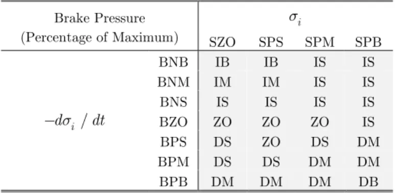
In this method, a fuzzy controller is employed to control the WSPD (Cheok and Shiomi, 2000). The structure of this controller has been designed using the reference measured data and the experi-mental knowledge of experts. In this controller, the values of absolute slide and its derivative is chosen as the inputs of the system, and the maximum cylinder pressure (%) is considered as its output. By determining the membership functions of the system inputs and output in the form of Figure 5, the fuzzy rules are expressed as in Table 5. It should be noted that in this approach, de-duction based on separate rules, Max-Product rule implication, and the center average defuzzifica-tion method are used to reduce the computadefuzzifica-tional complexity. Now, the data is sampled and the achieved output is applied to the valves of the WSPD as the bandwidth of the PWM signal.
Figure 5: Membership functions of (a) absolute slide, (b) deceleration of wheel set and (c) the brake pressure in the Mitsubishi fuzzy controller (Cheok and Shiomi, 2000).
-1 0 1 2 3 4 5 6
(a) Absolute Slide (km/h) 1
0 SZ0
SPS SPM
SPB
-3 -1 1 3 5 7 9
(b) Deceleration of Wheel set (km/h/s) BNB
BNM BNS BZO BPS BPM
BPB
1
0
0 0.5 1
0 20 40 60 80 100
(c) Brake Pressure (Percentage of Maximum)
i
s Brake Pressure
(Percentage of Maximum) SZO SPS SPM SPB
IS IS IB IB BNB / i ds dt
-IS IS IM IM BNM IS IS IS IS BNS IS ZO ZO ZO BZO DM DS ZO DS BPS DM DM DS DS BPM DB DM DM DM BPB
Table 5: Fuzzy rules in the controller presented by Mitsubishi (Cheok and Shiomi, 2000).
It should be mentioned that, for implementing the common algorithms, data sampling is per-formed at 100 ms time intervals to generate the input for the WSPD. But by reviewing the afore-mentioned works, it is concluded that the stability of the heuristic knowledge-based methods have not been investigated at all. It should be mentioned that fuzzy control method has been used for tire antilock braking systems in vehicles (Moallem et al., 2006; Cabrera et al., 2005).
5 SYSTEM CONTROL BY MEANS OF SLIDING-MODE METHOD
By taking the derivative of (3) and using (1) and (2), the equation for the changes of the longitudi-nal slip ratio of the wheel sets is obtained.
2
) )
0.5 ( ( , ) 8 (
( , ) ( )
brake W W fr x d fr x
W W
x
W x brake
T B R f f v t f
R R
v I v m
F t GT t
w l w l
l
l
é- - + ù é- - ù
- ê ú ê ú
= ê ú+ ê ú
ê ú ê ú
ë û ë û
= +
(19)
In the above equation, the braking torque is considered as the input of the system, and the lon-gitudinal slip ratio is taken as its output. Now by assuming uncertainties in the system structure such as severe changes in the friction, the car masses, and inertia properties, the above equation will be written as
( , ) ( , ) ( , ) ( ) ( , ) ( ) ( ) , ) ( ( )
x x x brake
x brake x brake x brake
F t F t G G T
F t GT t F t GT t F t GT t
t
l l l
l l l d
é ù é ù
=ë + D û+ë + D û
é ù
= + + Dë + D û = + +
(20)
To design the sliding-mode controller, it is assumed that d £W. By defining the tracking
er-ror and the sliding surface of the wheel sets as
( ) ( )
x x x
e t d t
l =l -l (21)
0
( ) ( ) ( ) , , 0
t
P x I x P I
e e
s t =K l t +K
ò
l t td K K > (22)( ) eq( ) ht( )
u t =u t +u t
(
)
1
( ) ( , ) ( ) / ( )
eq x x I P x
d e
u t =G- êé-F l t +l t + K K l t ùú
ë û
1
( ) . ( ( ) / )
ht
u t =G- éëW sat s t F ùû
(23)
Where the equivalent control term ueq is obtained by s =0 and the robust control term uht
compensates the uncertainties effect. In the designed sliding-mode controller, ueq is a function of F
and G (Equation (23)). Therefore, ueq is computed using the values of friction coefficient and the
locomotive parameters. In the SMC, the uncertainty upper bound W , which include the unknown
dynamics and parameter variations, must be available. However, it is difficult to obtain W for the
plant. The disadvantages of the SMC are fully dependency on dynamic model and the need for
un-certainty upper bound W .
Chattering phenomena can be improved by using satfunction instead of sgn. It should be
men-tioned that the boundary layer thickness of sat function is equal to F. By choosing the Lyapunov
function as
2
1 2
V = s (24)
In the case in which sat function is equal to sgnfunction (outside the boundary layer), the
de-rivative of V is written as belows:
( ) ( / )
( ) 0
P x I x P
e e
P P P P P
V s s s K K K s W s s
K s K W s K s K W s K W s
l l d
d d d
= ´ = ´ + = ´
-= - ´ - £ ´ - = - - £
(25)
Thus, the designed sliding-mode controller will ensure the stability of the system according to the Lyapunov stability criterion (Slotine and Li, 1991). Now, to apply the input to the actuator, the computed torque must be converted to its corresponding bandwidth.
( ) ( )
brake max
u t dc t
T
= (26)
6 PROPOSED ADAPTIVE FUZZY SLIDING-MODE CONTROLLER
By assuming all the parameters of the system (19) to be known, the ideal control input u* is
ob-tained from the following equation:
* 1 ( , ) ( ) I ( )
x x x
d e
P K
u G F t t t
K
l l l
- éê ùú
= ê- + + ú
ë û
(27)
( ) I ( ) 0
x x
e e
P K
t t
K
l + l = (28)
Since the implementation of u* is not practically possible, the ideal control input is
approxi-mated by an ideal fuzzy system ufuz. Thus, there is no need to determine the values of friction
forc-es and the locomotive parameters. After choosing a sliding surface such as (22), a Takagi-Sugeno
(TS) fuzzy system with sliding surface input s and output ufuz is considered as follows:
Rule r: If s is equal to Ar, then ufuz will be equal to br (r = 1,…, nr).
r
b is the fuzzy singleton output associated with rule r, and Ar is a fuzzy set, determined
itera-tively by a Gaussian membership function, as follows:
2
( ) exp
r
r r
A
s c
s m
s
é æ ö ù -ê ç ÷÷ ú = êê-çççè ÷÷÷ø úú
ê ú
ë û
(29)
Figure 6: Membership functions for the sliding surface input.
In the above equation, cr and sr denote the center and width of a membership function,
re-spectively. The selected membership functions are shown in Figure 6. By employing the singleton fuzzifier, the product inference, and the center average defuzzifier, the output of the fuzzy system is obtained as
1
1
( )
( )
n r r
r
fuz r A
n r
r r A
b s
u
s m
m
=
= =
å
å
(30)By defining the rule r as
1
( )
, 1, , ,
( )
r
r A
r n
r r r A
s
w r n
s m
m
=
= = ¼
å
(31)-0.4 -0.2 0 0.2 0.4 0.6
0 0.2 0.4 0.6 0.8 1
s
M
em
be
rs
hi
p
D
egre
e
Zero
PB
the output of the fuzzy system will be rewritten as (32).
1 1
( , ) , , , , , ,
T T
n n
fuz T r r
u s = = êéb ¼¼b úù = êéw ¼¼w ùú
ë û ë û
b b w b w (32)
Now, by considering the approximation error x, the ideal controller u* can be estimated from
the following equation:
* fuz T
u =u + =x b w+x (33)
The approximation error is presumed to be bounded.
x £y (34)
Since the optimal values of b and y may not be practically known, therefore adaptive method
is used to its evaluation. So, uˆfuz is presented for approximating ideal controller u*.
ˆ ˆ
ˆ ( , )fuz T
u sb =b w (35)
In the above equation, bˆ is the estimated value of vector b. Now, the system input is
consid-ered as
( , ˆ
ˆfuz ) r( )
u =u sb +u s (36)
where controller ur compensates the difference between the ideal and fuzzy controllers, and it is
computed from the following equation:
( ) )
ˆ (
r
u =ysgn s sgn G (37)
It should be mentioned that yˆ is the estimated limit of the fuzzy approximation error. To
overcome adverse effect of chattering phenomena, sat s( ) is used instead of sgn s( ). Now, by
substi-tuting (36) into (19), the following relation is obtained.
ˆ
( , ) (ˆfuz( , ) r( ))
x F x t G u s u s
l = l + b + (38)
Thus, by adding the above equation with the product of (27) and G (with regards to (21) and
(22)), the dynamic equation of the tracking error is obtained as follows:
*
( ) I ( ) ( ˆfuz( ,ˆ) r( ))
x x
e P e P
K s
t t G u u s u s
K K
l + l = - b - = (39)
Now, by defining the approximation errors as
ˆ
= -
b b b
ˆ
( )t ( )t
y = y-y
* ˆ
fuz fuz T
u =u -u =b w +x
the adaptation algorithms are expressed as (41) and (42).
1
ˆ = - = as
b b w (41)
2 ( )
ˆ s sgn G
y = - =y a (42)
In the adaptation algorithms, a1 and a2 are the adaptation rates and they are selected as
posi-tive constant numbers. The structure of the adapposi-tive fuzzy sliding-mode controller is shown in Fig-ure 7. Now, to evaluate the stability of the system in the presence of the designed controller, the following positive definite function is considered as the Lyapunov function:
2 2
2
1 2
1 ( , , )
2 2 2
T P
G G
V s s
K
y y
a a
= + +
b b b (43)
Figure 7: The structure of the adaptive fuzzy sliding-mode controller.
By taking the derivative of V s2( , , )b y with respect to time and considering (37) through (42),
2
1 2 1 2
1 2
( , , ) ( )
( )
( ) 0
T T r T
P
T r
ss G G G G
V s sG u
K
G
G s sG u sG s G s G s G
s G
y yy x yy
a a a a
x yy x y x y
a a
y x
= + + = + - + +
æ ö÷
ç ÷
ç
= çç + ÷÷+ - + = - £
-÷
çè ø
= - - £
b b b b w b b
b
b w (44)
It is concluded that V s2( , , )b y is always negative semi-definite; indicating the stability of the
system according to the Lyapunov’s concept. Thus, all the parameters of y, b and s are bounded.
Barbalat’s Lemma is used to verify the convergence of the tracking error to zero (Poursamad and Markazi, 2009a). So by considering the following equation
2
( )t º s G (y- x)£ -V
Г (45)
Sliding surface (22)
Bound Estimation (42) Robust Controller
(37) Adaptation law
(41)
Fuzzy Controller
(35) Plant (19)
+
+ +
-
s Bandwidth
and integrating Г( )t with respect to time, the following equation is obtained:
2 2
0
( ) ( (0), , ) ( ( ), , )
t
d V s V s t
t t £ y - y
ò
Г b b (46)Since V s2( (0), , )b y is bounded and
2( ( ), , )
V s t b y is non-increasing and bounded, (47) is written
as follows.
0
lim ( )
t
t¥
ò
Гt td £¥ (47)So considering Barbalat’s Lemma, Equation (48) is obtained.
lim ( ) lim ( ) 0
t¥Гt =t¥s t = (48)
Thus, the tracking error converges to zero, and the system becomes asymptotically stable.
7 SIMULATION RESULTS
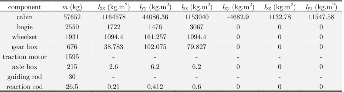
To demonstrate the performance of the proposed control strategy, the adaptive fuzzy sliding-mode controller is applied to the wheel slide protection device for numerical simulations. In addition, for the purpose of comparison, Trenitalia, Knorr-Bremse, and Mitsubishi control techniques are imple-mented. To consider the effects of unmodeled movements during the controller design, the multi-body dynamics method is used for simulating the longitudinal dynamics of ER24PC locomotive (Figure 8). In the simulations, the weight shifting is considered during braking. It should be men-tioned that the modeled locomotive with 82 degrees of freedom, has been validated using the test data provided by Mapna Locomotive and Siemens Companies. The values of parameters, degrees of freedom, and masses and inertia properties of the components of the locomotive are presented in
Tables 6, 7 and 8, respectively. Also, the constant values of a and b are considered based on
Po-lach (1999). The initial velocity of the locomotive is assumed to be 120 km/h.
To compare the performance of the controllers in the presence of uncertainties, random track ir-regularities are considered. To generate the irir-regularities, Power Spectral Densities (PSDs) obtained from measurement data are used. The PSDs for horizontal, vertical and lateral track irregularities
are defined in ERRI B176 (SIMPACK AG, 2016). With the wavenumber W and the wavelength
L , the analytical representation of the PSDs Strack is defined as Equation (49).
2
0 2
2 4 6
0 2 4 6
2
( ) ,
track S
L
b b p
g g g g
+ W
W = W =
Figure 8: Multi-body dynamics modelling of ER24PC locomotive during braking.
parameter value unit
mass of locomotive 76841 kg
wheelbase 2700 mm
track gauge 1435 mm
wheel diameter 1100 mm
track cant 1:40 -
Young’s modulus 210 GPa
Poisson’s ratio 0.25 -
cmax
P 6 bar
TF 0.6 s
TV 0.6 s
brakemax
T 60 kNm
Table 6: Values of parameters in modelling of ER24PC locomotive.
total degrees of freedom number of component
component
6 1
Locomotive body
12 2
bogie frame
24 4
wheelset
8 8
axlebox
4 4
traction rod
4 4
gearbox
24 8
steering rod
Table 7: Total degrees of freedom of ER24PC locomotive components.
component m (kg) Ixx (kg.m2) Iyy (kg.m2) Izz (kg.m2) Ixy (kg.m2) Ixz (kg.m2) Iyz (kg.m2)
cabin 57652 1164578 44086.36 1153040 -4682.9 1132.78 11547.58
bogie 2550 1722 1476 3067 0 0 0
wheelset 1931 1094.4 161.257 1094.4 0 0 0
gear box 676 38.783 102.075 79.827 0 0 0
traction motor 1595 - - - -
axle box 215 2.6 6.2 6.2 0 0 0
guiding rod 30 - - - -
reaction rod 26.5 0.21 0.412 0.6 0 0 0
According to EN 13848-1:2003+A1:2008 (2009), for typical track irregularities in the public
transportation, the wavelength is chosen in the range of 3m £L£25m. Also, the PSD coefficients
(b0 to b2 and g0 to g6) are chosen based on Table 9.
Due to the vibration of the brake pads at the onset of braking, the disturbing torque
0.05 exp( 4 ) (10 )
d brake
T = T - t sin pt is added to the braking torque. The initial output values of the
membership functions, and the uncertainty limit are chosen as bˆ= - -[ 1, 0.5, 0, 0.5,1]T and y =1,
respectively. Also, the controller parameters are specified as a1 =10, a2 =0.85, KI =550 and
1800
P
K = .
0
b (.10-7) b2 (.10-6) g0 (.10-4) g2 g4 g6
Horizontal excitation 4.164787 0 2.8855 0.68038 1 0
Vertical excitation 7.343623 0 2.8855 0.68038 1 0
Lateral excitation 0 0.305533 0.55356 0.13081 0.8722335 1
Table 9: PSD coefficients for the track-irregularities.
By applying Trenitalia, Knorr-Bremse and Mitsubishi methods for different frictional condi-tions, the diagrams of wheel sets slip ratios and velocities are plotted. In view of Figures 9 and 10, when using Trenitalia method, it is seen that the slip ratios and velocities go beyond the specified range (according to (16)). Due to the decrease of the locomotive velocity, the wheel sets slip ratios diverge near the stopping time. It should be mentioned that severe fluctuations in the wheel sets velocities will reduce the service life of the frictional parts involved (Barna, 2012). As shown in Fig-ures 11 and 12, in comparison with FigFig-ures 9 and 10, the fluctuations of the slip ratios and veloci-ties have been decreased by using Knorr-Bremse technique. The diagrams of the wheel sets slip ratios and velocities resulted from using Mitsubishi controller are presented in Figures 13 and 14, respectively. As shown in Figure 13, when applying Mitsubishi controller with braking on dry rails, the wheel sets slip ratios don’t exceed 0.3; while in the case of braking on wet rails, the slip ratios of the wheel sets fluctuate and eventually diverge. It is concluded that the performance of Mitsubishi method is affected in different frictional conditions.
Figure 9: Slip ratio of wheel sets in the case of braking on (a) dry rails, and (b) wet rails, and by using the controller devised by Trenitalia.
0 2 4 6 8
0 0.2 0.4 0.6 0.8 1
Time(s)
Sl
ip
Ra
tio
Lower Bound of Slip Ratio Upper Bound of Slip Ratio Wheelset1 Slip Ratio Wheelset2 Slip Ratio Wheelset3 Slip Ratio Wheelset4 Slip Ratio
(a)
0 2 4 6 8 10 12
0 0.2 0.4 0.6 0.8 1
Time(s)
Sl
ip
Ra
tio
Lower Bound of Slip Ratio Upper Bound of Slip Ratio Wheelset1 Slip Ratio Wheelset2 Slip Ratio Wheelset3 Slip Ratio Wheelset4 Slip Ratio
Figure 10: Velocity of wheel sets and locomotive in the case of braking on (a) dry rails, and (b) wet rails, and by using the controller devised by Trenitalia.
Figure 11: Slip ratio of wheel sets in the case of braking on (a) dry rails, and (b) wet rails, and by using the controller presented by Knorr-Bremse.
Figure 12: Velocity of wheel sets and locomotive in the case of braking on (a) dry rails, and (b) wet rails, and by using the controller presented by Knorr-Bremse.
0 2 4 6 8
0 20 40 60 80 100 120 Time(s) V el oc ity (k m /h ) Locomotive Wheelset1 Wheelset2 Wheelset3 Wheelset4 Velocity lower bound Velocity upper bound (a)
0 2 4 6 8 10 12
0 20 40 60 80 100 120 Time(s) V el oc ity (k m /h ) Locomotive Wheelset1 Wheelset2 Wheelset3 Wheelset4 Velocity lower bound Velocity upper bound (b)
0 2 4 6 8 10
0 0.2 0.4 0.6 0.8 1 Time(s) Sl ip R at io
Desired Slip Ratio Wheelset1 Slip Ratio Wheelset2 Slip Ratio Wheelset3 Slip Ratio Wheelset4 Slip Ratio (a)
0 2 4 6 8 10 12
0 0.2 0.4 0.6 0.8 1 1.2 Time(s) Sl ip R at io
Desired Slip Ratio Wheelset1 Slip Ratio Wheelset2 Slip Ratio Wheelset3 Slip Ratio Wheelset4 Slip Ratio
(b)
0 2 4 6 8 10
0 20 40 60 80 100 120 Time(s) V el oc ity (km /h ) Locomotive Wheelset1 Wheelset2 Wheelset3 Wheelset4 (a)
0 2 4 6 8 10 12
Figure 13: Slip ratio of wheel sets in the case of braking on (a) dry rails, and (b) wet rails, and by using the controller presented by Mitsubishi.
After applying the AFSM controller in different frictional conditions, the diagrams of the wheel sets slip ratios and velocities are presented in Figures 15 and 16, respectively. As is shown in Figure 15, in both frictional conditions, the wheel sets slip ratios fluctuates about the desired value of 0.14. Of course, at the end of braking, due to the reduction of the locomotive velocity, the amplitude of the slip ratios oscillations increases. It should be noted that in the case of braking on wet rails, the settling time of the slip ratios reduces. Also, as observed in Figure 16, by using the AFSM control-ler, the amplitude of the velocities fluctuations is low in comparison with the other approaches. So, the simulation results show that in comparison with Trenitalia and Knorr-Bremse techniques, AFSMC method can overcome the divergence of wheel sets slip ratios near the stopping time. Also, in comparison with Mitsubishi controller, AFSM controller can improve the robustness of the WSPD regarding various rail conditions.
Wheel set1 braking torque with braking on dry and wet rails and using Trenitalia, Knorr-Bremse, and Mitsubishi controllers are presented in Figures 17 and 18, respectively. Also, using the AFSM controller, wheel set1 input and braking torque in the case of braking on dry and wet rails and are shown in Figures 19 and 20, respectively. As seen in Figures 17-20, in the case of braking on wet rails, the frequency of input (braking torque) fluctuations increases. Also, the lowest and the highest switching frequency of the braking torque are related to Trenitalia and Mitsubishi methods. It should be mentioned that using AFSM controller, the switching frequency of the actuator input is in the allowed range regarding the common sampling time interval (=100 ms).
Figure 14: Velocity of wheel sets and locomotive in the case of braking on (a) dry rails, and (b) wet rails, and by using the controller presented by Mitsubishi.
0 2 4 6 8 10
0 0.05 0.1 0.15 0.2 0.25 0.3 Time(s) Sl ip R at io
Desired Slip Ratio Wheelset1 Slip Ratio Wheelset2 Slip Ratio Wheelset3 Slip Ratio Wheelset4 Slip Ratio (a)
0 2 4 6 8 10 12
0 0.2 0.4 0.6 0.8 1 Time(s) Sl ip R at io
Desired Slip Ratio Wheelset1 Slip Ratio Wheelset2 Slip Ratio Wheelset3 Slip Ratio Wheelset4 Slip Ratio (b)
0 2 4 6 8 10
0 20 40 60 80 100 120 Time(s) V el oc ity (k m /h) Locomotive Wheelset1 Wheelset2 Wheelset3 Wheelset4 (a)
0 2 4 6 8 10 12
Figure 15: Slip ratio of wheel sets in the case of braking on (a) dry rails, and (b) wet rails, and by employing the adaptive fuzzy sliding-mode controller.
Figure 16: Velocity of wheel sets and locomotive in the case of braking on (a) dry rails, and (b) wet rails, and by employing the adaptive fuzzy sliding-mode controller.
At the end, the integral of wheel sets braking torque, the distance and time taken to stop the locomotive in each of the conditions are presented in Table 10. As shown in Table 10, by applying the AFSMC method, the stopping time and the braking distance of the locomotive have been de-creased regarding various rail conditions. According to Equation (12), the amount of a wheel set braking torque is proportional to the pressure of the corresponding cylinder. Thus, as stated in Petrenko (2017) and EN 15595 (2011), the air consumption of the braking system can be evaluated
0 1 2 3 4 5 6 7 8 9
0 0.05 0.1 0.15 0.2 0.25 0.3 0.35
Time(s)
Sl
ip
R
at
io
Desired Slip Ratio Wheelset1 Slip Ratio Wheelset2 Slip Ratio Wheelset3 Slip Ratio Wheelset4 Slip Ratio
(a)
0 2 4 6 8 10 12
0 0.05 0.1 0.15 0.2 0.25 0.3 0.35
Time(s)
Sl
ip
R
at
io
Desired Slip Ratio Wheelset1 Slip Ratio Wheelset2 Slip Ratio Wheelset3 Slip Ratio Wheelset4 Slip Ratio (b)
0 2 4 6 8
0 20 40 60 80 100 120
Time(s)
V
el
oc
ity(km
/h)
Locomotive Wheelset1 Wheelset2 Wheelset3 Wheelset4 (a)
0 2 4 6 8 10 12
0 20 40 60 80 100 120
Time(s)
V
el
oc
ity(km
/h)
using the value of 4 0 1 stop t brake i i T dt =
ò
å
. In the case of braking on dry rails and employing AFSMcon-troller, the integral of wheel sets braking torque increases in comparison with the other control techniques.
Figure 17: Wheel set1 braking torque in the case of braking on dry rails and using (a) Trenitalia, (b) Knorr-Bremse, and (c) Mitsubishi controllers.
4 1 0 stop t brakei i T dt =
ò
å
(kNm.s)stopping time (s) braking distance (m)
control method wet rail dry rail wet rail dry rail wet rail dry rail 1564.66 1572.48 12.3 9.9 221.15 184.63 Trenitalia 1576.44 1570.26 13.1 10.5 246.68 207.37 Knorr-Bremse 1570.31 1556.8 12.8 10.5 235.33 201.40 Mitsubishi 1565.84 1578.03 12.2 9.8 220.60 184.03 AFSMC
Table 10: Comparing simulation results obtained by assuming an initial locomotive speed of 120 km/h.
While the value of 4 0 1 stop t brake i i T dt =
ò
å
decreases in the case of braking on wet rails.In Figure 21, the comparison of vertical forces exerted on two different wheel sets in the case of braking on wet rails (and using the AFSMC method) is shown. It can be realized that due to con-sidering the 3D body dynamics in the co-simulation method, vertical forces exerted on different wheel sets are not equal. So, in the simulations, the weight shifting will happen during braking. As shown in Figures 15 and 16, this phenomenon causes differences between the slip ratios and
veloci-0 2 4 6 8
0 2 4 6x 10⁴
Time(s) W he el se t1 B ra ki ng Torq ue (N m ) (a)
0 2 4 6 8 10
0 2 4 6x 10⁴
Time(s) W he el se t1 Br aki ng To rq ue (N m ) (b)
0 2 4 6 8 10
0 2 4 6x 10
ties of front wheel sets (wheel sets 3 and 4) and rear wheel sets (wheel sets 1 and 2). It should be noted that, despite the different values of the normal forces, the slip ratios of the front and rear wheel sets converge towards the desired value.
Figure 18: Wheel set1 braking torque in the case of braking on wet rails and using (a) Trenitalia, (b) Knorr-Bremse, and (c) Mitsubishi controllers.
Figure 19: Wheel set1 (a) WSPD input and (b) braking torque in the case of braking on dry rails and by employing the adaptive fuzzy sliding-mode controller.
If large creepages between wheels and rails have a high endurance, the dissipation of energy at the rolling surfaces increases considerably. This phenomenon can lead to wheel/rail wear. In this work, the performed simulations and the obtained results are in accordance with the guidelines of EN 15595 (2011). In the guidelines of EN 15595 (2011), limits are set regarding the locking and the maximum absolute slide of the wheel sets. This standard covers the system acceptance requirements as well as the application specific requirements for wheel slide protection systems.
0 2 4 6 8 10 12
0 1 2 3 4
x 104
Time(s) W he el se t1 B ra ki ng To rq ue (N m ) (a)
0 2 4 6 8 10 12
0 1 2 3 4x 10
4 Time(s) W he el se t1 B ra ki ng To rq ue (N m ) (b)
0 2 4 6 8 10 12
0 1 2 3 4x 10⁴
Time(s) W he el se t1 B ra ki ng To rq ue (N m ) (c)
0 2 4 6 8
-1 0 1 2 Time(s) A ct ua tor1 Inp ut (a)
0 2 4 6 8
0 2 4 6x 10
8 CONCLUSIONS
In this study, an adaptive fuzzy sliding-mode PWM controller is designed for the WSPD of ER24PC locomotive to regulate the wheel sets slip ratios in the presence of uncertainties with un-known bounds. On the contrary to the heuristic and knowledge-based techniques, no reference measured data and the experimental knowledge of relevant experts is needed for designing AFSM controller. The second Lyapunov theorem, guarantees the convergence of the slip ratio to the de-sired values. Unlike the SMC method which needs a relatively accurate model of the plant to guar-antee the stability, the AFSMC method needs minimal information from the model of the plant. The reason is that the upper bound of the plant uncertainty is estimated online by the proposed method. This feature, furthermore, prevents excessive switching of the control input which is a common phenomenon in the conventional SMC methods.
Figure 20: Wheel set1 (a) WSPD input and (b) braking torque in the case of braking on wet rails and by employing the adaptive fuzzy sliding-mode controller.
Figure 21: Comparison of vertical forces exerted on different wheel sets in the case of braking on wet rails and by employing the adaptive fuzzy sliding-mode controller.
Multi-body dynamics model for simulation of the longitudinal dynamics of the ER24PC locomo-tive is employed. The model is consisting 82 degrees of freedom. The model has been validated us-ing the test data provided by Mapna Locomotive and Siemens Companies. The simulation results depict that, in comparison with Trenitalia, Knorr-Bremse and Mitsubushi techniques, AFSMC method can improve the robustness of the WSPD regarding various rail conditions. It should be
0 2 4 6 8 10 12
-1 0 1 2
Time(s)
A
ct
ua
tor1
Inp
ut
(a)
0 2 4 6 8 10 12
0 1 2 3 4 5x 10
4
Time(s)
W
he
el
se
t1
B
ra
ki
ng
To
rq
ue
(N
m
) (b)
2 4 6 8 10 12
0 50 100 150 200
Time(s)
V
ert
ic
al
W
he
el
F
or
ce
(kN
mentioned that by applying the AFSMC method, the stopping time and the braking distance of the locomotive have been decreased, while only a minimum amount of information of the plant is em-ployed in the control design process.
Acknowledgment
The authors would like to thank Mapna Locomotive Company, and in particular, Eng. Fazli, for providing the test data used to evaluate the accuracy of locomotive model. This research did not receive any specific grant from funding agencies in the public, commercial, or not-for-profit sectors.
References
Anwar, S., Zheng, B., (2007). An Antilock-Braking Algorithm for an Eddy-Current-Based Brake-By-Wire System. IEEE TRANSACTIONS ON VEHICULAR TECHNOLOGY 56(3): 1100-1107.
Barna, G., (2012). Matlab Simulink(r) Model of a Braked Rail Vehicle and Its Applications. Technology and Engi-neering Applications of Simulink. P. S. Chakravarty, InTech.
Bhandari, R., Patil, S., Singh, R.K., (2012). Surface prediction and control algorithms for anti-lock brake system. Transportation Research Part C: Emerging Technologies 21(1): 181-195.
Cabrera, J.A., Ortiz, A., Castillo, J.J., Sim'on, A., (2005). A Fuzzy Logic Control for Antilock Braking System Inte-grated in the IMMa Tire Test Bench. IEEE TRANSACTIONS ON VEHICULAR TECHNOLOGY 54(6): 1937-1949.
CEN, (2009). EN 13848-1:2003+A1:2008, Railway applications -Track -Track geometry quality -Part 1: Characteri-sation of track geometry.
CEN, (2011). EN 15595, Railway applications-Braking - Wheel slide protection.
Cheok, A.D., Shiomi, S., (2000). Combined Heuristic Knowledge and Limited Measurement Based Fuzzy Logic Anti-skid Control for Railway. IEEE TRANSACTIONS ON SYSTEMS, MAN, AND CYBERNETICS-PART C: AP-PLICATIONS AND REVIEWS 30.
Cocci, G., Presciani, P., Rindi, A., Volterrani, G.P.J., (2001). Railway Wagon Model with Anti-slip Braking System. 16th European MDI User Conference. Berchtesgaden, Germany.
Colombo, E.F., Di Gialleonardo, E., Facchinetti, A., Bruni, S., (2014). Active carbody roll control in railway vehicles using hydraulic actuation. Control Engineering Practice 31: 24-34.
FAIVELEY, (2010). FAIVELEY BRAKE SYSTEM-Wheel Slide Protection System.
Gholami, A., Markazi, A.H.D., (2012). A new adaptive fuzzy sliding mode observer for a class of MIMO nonlinear systems. Nonlinear Dynamics 70(3): 2095–2105.
Harifi, A., Aghagolzadeh, A., Alizadeh, G., Sadeghi, M., (2008). Designing a sliding mode controller for slip control of antilock brake systems. Transportation Research Part C: Emerging Technologies 16(6): 731-741.
Ho, H., Wong, Y., Rad, A., (2009). Adaptive fuzzy sliding mode control with chattering elimination for nonlinear SISO systems. Simulation Modelling Practice and Theory 17: 1199–1210.
Hwang, C.-L., Kuo, C.-Y., (2001). A Stable Adaptive Fuzzy Sliding-Mode Control for Affine Nonlinear Systems with Application to Four-Bar Linkage Systems. IEEE TRANSACTIONS ON FUZZY SYSTEMS 9.
Jing, H., Liu, Z., Chen, H., (2011). A Switched Control Strategy for Antilock Braking System With On/Off Valves. IEEE TRANSACTIONS ON VEHICULAR TECHNOLOGY 60(4): 1470-1484.
Khazaee, M., Markazi, A.H.D., Omidi, E., (2015). Adaptive fuzzy predictive sliding control of uncertain nonlinear systems with bound-known input delay. ISA Transactions 59: 314–324.
Kim, J.S., Park, S.H., Choi, J.J., Yamazaki, H.-O., (2011). Adaptive Sliding Mode Control of Adhesion Force in Railway Rolling Stocks. Sliding Mode Control, InTech.
Leva, S., Morando, A.P., Colombaioni, P., (2008). Dynamic Analysis of a High-Speed Train. IEEE TRANSAC-TIONS ON VEHICULAR TECHNOLOGY 57(1): 107-119.
Lhee, C.-G., Park, J.-S., Ahn, H.-S., Kim, D.-H., (2001). Sliding Mode-Like Fuzzy Logic Control with Self-Tuning the Dead Zone Parameters. IEEE TRANSACTIONS ON FUZZY SYSTEMS 9: 343-348.
Li, P., Goodall, R., Weston, P., Ling, C.S., Goodman, C., Roberts, C., (2007). Estimation of railway vehicle suspen-sion parameters for condition monitoring. Control Engineering Practice 15(1): 43-55.
Lin, C.-M., Hsu, C.-F., (2003). Self-Learning Fuzzy Sliding-Mode Control for Antilock Braking Systems. IEEE TRANSACTIONS ON CONTROL SYSTEMS TECHNOLOGY 11: 273-278.
Meli, E., Pugi, L., Ridolfi, A., (2014). An innovative degraded adhesion model for multibody applications in the railway field. Multibody System Dynamics 32(2): 133–157. doi:10.1007/s11044-013-9400-9.
Meli, E., Ridolfi, A., (2015). An innovative wheel–rail contact model for railway vehicles under degraded adhesion conditions. Multibody System Dynamics 33(3): 285–313. doi:10.1007/s11044-013-9405-4.
Mirzaei, A., Moallem, M., Dehkordi, B.M., Fahimi, B., (2006). Design of an Optimal Fuzzy Controller for Antilock Braking Systems. IEEE TRANSACTIONS ON VEHICULAR TECHNOLOGY 55(6): 1725-1730.
Mirzaei, M., Mirzaeinejad, H., (2012). Optimal design of a non-linear controller for anti-lock braking system. Trans-portation Research Part C: Emerging Technologies 24: 19-35.
Mirzaeinejad, H., Mirzaei, M., (2010). A novel method for non-linear control of wheel slip in anti-lock braking sys-tems. Control Engineering Practice 18(8).
Mirzaeinejad, H., Mirzaei, M., (2014). Optimization of nonlinear control strategy for anti-lock braking system with improvement of vehicle directional stability on split-μ roads. Transportation Research Part C: Emerging Technolo-gies 46: 1-15.
Patil, A., Ginoya, D., Shendge, P.D., Phadke, S.B., (2016). Uncertainty-Estimation-Based Approach to Antilock Braking Systems. IEEE TRANSACTIONS ON VEHICULAR TECHNOLOGY 65(3): 1171-1185.
Petrenko, V., (2017). Railway Rolling Stock Compressors Capacity and Main Reservoirs Volume Calculation Meth-ods. Paper presented at the 10th International Scientific Conference Transbaltica 2017: Transportation Science and Technology, Vilnius Gediminas Technical University.
Polach, O., (1999). A Fast Wheel-Rail Forces Calculation Computer Code.
Polach, O., (2005). Creep forces in simulations of traction vehicles running on adhesion limit. Wear 258: 992–1000. Poursamad, A., Markazi, A.H.D., (2009a). Robust adaptive fuzzy control of unknown chaotic systems. Applied Soft Computing 9(3): 970–976.
Poursamad, A., Markazi, A.H.D., (2009b). Adaptive fuzzy sliding-mode control for multi-input multi-output chaotic systems. Chaos, Solitons and Fractals 42(5): 3100–3109.
Pugi, L., Malvezzi, M., Tarasconi, A., Palazzolo, A., Cocci, G., Violani, M., (2006). HIL simulation of WSP systems on MI-6 test rig. Vehicle System Dynamics, 44(sup1): 843–852. doi:10.1080/00423110600886937.
Pugi, L., Grasso, F., Pratesi, M., Cipriani, M., Bartolomei, A., (2017). Design and preliminary performance evalua-tion of a four wheeled vehicle with degraded adhesion condievalua-tions. Internaevalua-tional Journal of Electric and Hybrid Vehi-cles 9(1): 1-32. doi:10.1504/IJEHV.2017.10003707.
Shim, T., Chang, S., Lee, S., (2008). Investigation of Sliding-Surface Design on the Performance of Sliding Mode Controller in Antilock Braking Systems. IEEE TRANSACTIONS ON VEHICULAR TECHNOLOGY 57(2): 747-759.
SIMPACK AG., (2016). Simpack Documentation, Release 9.9.2.
Song, Q., Song, Y., (2010). Adaptive Control and Optimal Power/Brake Distribution of High Speed Trains with Uncertain Nonlinear Couplers. Proceedings of the 29th Chinese Control Conference, Beijing, China.
Tong, S., Li, H.-X., (2003). Fuzzy Adaptive Sliding-Mode Control for MIMO Nonlinear Systems. IEEE TRANSAC-TIONS ON FUZZY SYSTEMS 11: 354-360.