Abstract
An approach is suggested in this paper that has successfully been applied in physics, ecology, and the biomedical sciences. This is called fractal-complex-adaptive-system (FCAS) modeling. The objective of this type of analysis is to reconstruct the dynamics of the pathological process that has been leading to the disease. Diabetes, a complexdisease, has been used to test the methodology. Biometrical analyses were undertaken on subjects diagnosed with overt diabetes (hereafter called IDDM), chemical diabetes (NIDDM), and a group of normal subjects. The studied variables were plasma glucose, insulin concentration, and insulin sensitivity. FCAS modeling con-sists in fitting a power-law function to the bivariate lognormal distribution of the vari-ables. The power-law exponent is estimated by principal component analysis (PCA). Analyses have shown that glucose disposal can be considered a fractal process, thereby implying a complex hierarchy of interact-ing scales and mechanisms in glucose han-dling. The first principal component repre-sents quantitative glucose disposal, and the second component is compatible with in-sulin efficiency. PCA further retrieved dis-tinct ongoing pathological processes within clinical groups of subjects. The IDDM in-sulin production defect had a high (abso-lute value) exponent of -3.5 that confirms a crude defect scanning the whole fractal hi-erarchy. Definite insulin resistance has been detected in clinically normal subjects with a low exponent of -0.5, thus suggest-ing a subtle and complex problem possibly due to aging or reduced physical activity. Insulin sensitivity was definitely impaired in the NIDDM clinical group with an expo-nent of -2.2, thereby suggesting poorly scheduled insulin feedback, possibly due to peripheral insensitivity. NIDDM appeared to result from aggravation of the subtle in-sensitivity seen in normal subjects. On the whole, the fractal model seemed to be ca-pable of assessing the degree of complexity of a disease. It is concluded that future
stud-The complex dynamics of
diabetes modeled as a fractal
complex-adaptive-system (FCAS)
A complexa dinâmica do diabetes
modelado como um sistema fractal
complexo adaptativo(FCAS)
Pierre Philippe
Department of Social and Preventive Medicine Faculty of Medicine, University of Montreal
M. d’Youville Bldg., PO Box. 6128, Station “A”,
Montreal H3C 3J7, QC, Canada Email: [email protected]
Bruce J. West
Department of Physics Center for Nonlinear ScienceP.O. Box 305370,
Denton, TX 76203-5370
ies of diabetes using FCAS modeling ought to be undertaken on the basis of multiple-scale biological variables, thereby closely reflecting the complexity of glucose han-dling. It is further recommended that such analyses be undertaken with dynamic data to track down the precise timing of the vari-ous homeostatic disruptions. It would also be important to carry out this type of analy-sis on less known but equally complex dis-ease processes. The results might point to important new research findings.
Keywords Keywords Keywords Keywords
Keywords: Power law. Fractals. Diabetes mellitus, insulin-dependent. Diabetes mel-litus, non-insulin dependent. Nonlinear dy-namics. Principal component analysis. Complex-adaptive-system modeling. Al-lometry
Resumo
feedback de insulina, provavelmente devi-do a insensibilidade periférica à insulina. O NIDDM parecia ser o resultado da piora da sutil insensibilidade encontrada entre os indivíduos normais. De modo geral, o mo-delo fractal provou ser capaz de avaliar o grau de complexidade da doença. Conclui-se, portanto, que estudos futuros do diabe-tes utilizando a modelagem FCAS devem ser realizados a partir de variáveis biológi-cas de escalas múltiplas, assim refletindo com exatidão a complexidade do proces-samento da glicose. Seria recomendável, ainda, que tais análises fossem realizadas com dados dinâmicos para investigar o momento preciso das diferentes alterações homeostáticas. Também seria importante realizar esse tipo de análise em processos patológicos menos conhecidos, mas igual-mente complexos. Esse resultados poderi-am levar a importantes novos achados de pesquisa.
Palavras-chave Palavras-chave Palavras-chave Palavras-chave
Palavras-chave: Modelos teóricos . Fractais. Diabetes mellitus não dependente. Diabetes mellitus insulino-dependente. Dinâmica não linear. Análise do componente principal. Modelagem de sistema adaptativo complexo. Alometria.
Introduction
Many epidemiologists are concerned with the current difficulty in understanding health and disease. On the one hand, risk-factor modeling (e.g., multivariate logistic regression) can fail to unravel the etiology
of complex disease processes1-3. For
ex-ample, the small percentage of the total variation in disease incidence typically ac-counted for by regression analyses is gen-erally taken as an indication of the failure
of structural modeleling4. On the other
hand, controversial findings are prevalent in epidemiology5-7. It is envisioned that the
future of epidemiology will establish even more inconsistencies. This is expected be-cause there will be an increased reliance on remote exposures (e.g., molecular epidemi-ology), the effects of which have to cross many scales of organization before produc-ing outcomes. There are two main reasons why causal research meets with limited suc-cess nowadays7; either some crucial
vari-ables remain hidden to the investigator do-ing risk-factor modeldo-ing or the underlydo-ing disease dynamics results requires a com-plex system approach at variance with risk-factor modeling. Our contention is not that risk-factor modeling should not be used, only that new approaches based on output of complex systems with nonlinear dynam-ics ought to be explored. This paper looks into systems with nonlinear dynamics.
Some investigators have already sug-gested that recourse to nonlinear dynam-ics can help unravel the web of causes (the black-box) that relates exposure to disease 2-4, 8,9. A few papers have established how the
presence of nonlinear dynamics in disease occurrence can, because of the non-inde-pendence of outcomes, jeopardize habitual analytical study designs2,3. Further,
at-tempts at modeling the black-box have been made; for example, one investigator has studied a nonlinear deterministic model of the incubation period8, and
neu-ral-nets have been used for clinical pattern
recognition10. These methods appear to
the early recognition of pathological pro-cesses.
In this paper, the nonlinear dynamics approach tested is called fractal-complex-adaptive-system (FCAS) modeling. FCAS models have been developed by research-ers from the Sante Fe Institute. Later, works related to FCAS but emphasizing their scal-ing or fractal nature have been carried out by a few investigators11-15. FCAS, by
defini-tion, is a hierarchy of multiple nonlinearly interrelated subsystems. FCAS models are useful whenever a phenomenon results from a signal that has been propagated through a comp lex hierarchy of scales of organization. The strength of FCAS is that it can identify the degree of smoothness or roughness of signal flow through the hierarchy. A well bro-ken-in FCAS entails a smooth mechanism that responds in an appropriate manner to the requirements of the outer world. A de-fective FCAS responds selfishly, i.e., it ignores the outer intervening systems or refrains from responding smoothly to subsystems. Therefore, smoothness of response involves spread-out correlations among subsystems and feedback. Health is equated with re-sponse smoothness. Disease, on the other hand, bears various degrees of roughness (interference in signal flow). The cruder the defect, the deeper in the hierarchy the dis-ease origin, and the more uncontrolled the mechanism (short-range or no correlations at all). Also, the deeper the disease origin, the more linear and the more obvious its rela-tion to a putative exposure. In contradistinc-tion, the more intricate the pathological pro-cess, the more nonlinear and the less pre-dictable its relation to any putative exposure. Because FCAS is complex and its com-ponents are interrelated by definition, the subsystem units and their interactions must be modeled together. Therefore, in order to assess the degree of complexity, one needs a global measure of the output of the hier-archical system. The reasoning is the follow-ing: if the output matches a given probabi-listic model (specific to FCAS), then the sytem is likely complex (as defined above). This approach is in contradistinction with
that of nonlinear risk-factor models such as multivariate regressions, that model the structure of interrelated observations on a nonlinear scale. The FCAS approach is not structural; it rather models the output of a complex system. Incidentally, the power-law function is specific to FCAS; the func-tion quantitatively assesses the envelope of the system. The operational methodology ensuing from the above viewpoint is two-fold. First, the health/disease process can be described by an evolving complex cova-riance structure of biological variables. Sec-ond, fractal geometry is useful in the study of biomedical phenomena with multiple scales of biological organization. The objec-tive of this paper is to test the validity of the FCAS approach in the study of a complex disease, diabetes. The conceptual founda-tions of FCAS in diabetes are reviewed in Appendix I.
Methods
Fractal objects can be identified with the aid of statistics. The signature of a fractal
object is a power-law function14,15. The
as a model for dynamics that are nonlinear should not be viewed as a defect for it has been shown that the envelope of experi-mental FCAS behaves that way15. The fractal
dimension (D) is related to the power-law exponent, ß, by the relation ß = 3-2D. More specifically, the more complex the studied phenomenon, the more spread out the cor-relations among scales.
In physical phenomena the power-law exponent of the power spectrum is often negative (inverse power law). The power-law exponent is an accurate assessment of the dispersion of the distribution14,15. A small
power-law exponent, between 0 and -2, re-fers to large dispersion and high complexity (no characteristic scale). A smaller power-law exponent indicates lower dispersion and points to a more straightforward phenom-enon. In other words, the smaller the inverse power-law exponent, the simpler, the more predictable, the more regular, and the more easily boxed-in is the process. These phe-nomena can successfully be investigated by linear methods. Contrariwise, the larger the value of the negative power-law exponent, the more complex, the more intricate, and the less easily boxed-in is the process. Lin-ear methods are useless here. This is the do-main of nonlinear dynamics. A power-law exponent of zero stands for white noise pro-cesses, i.e., chance phenomena with utter unpredictability. The mathematical under-pinnings of the principal component analy-sis (PCA) and the power law are detailed in Appendix II.
Caveats Caveats Caveats Caveats Caveats
Before embarking on the analysis per se, four issues deserve comment. First, diabe-tes can be considered a complex multiple-scale phenomenon. Accordingly, a cross-sectional sample of plasma measures of sufficient variability will embody the vari-ous scales of organization of the glucose regulation process of different subjects. Therefore, a cross-section of subjects from the same disease stage will reflect the com-plex dynamics of the latest pathological event. One can hope to reconstruct the
dy-namics of the latest pathological phase transition if it can be assumed that the mea-surement-specific biological variability is extended enough to cover the recent history of the disease process. More simply put, one uses a cross-section of various individuals as a surrogate for the individual disease pathway. In this context, the exponent of the allometric law becomes the expression for an observation of self-similarity in a se-ries of fractally structured individuals21.
Second, structural relationships of healthy phenomena are generally mea-sured by a positive power-law exponent. Accordingly, the disease state should be probed by a qualitative change in the cova-riance structure with respect to normalcy. Hence, the structure of a pathological pro-cess will translate to an “involuted” covari-ance structure leading to the reverse pat-terning of healthy relationships, and its measure will be an inverse power law.
The third issue to make clear is that PCA will break down the covariance structure into independent variables or dimensions, each having its own power-law exponent. This will occur if multiple sources (two here) of variation coexist. In the latter case, the second principal component, orthogonal to the first, will necessarily yield at least one inverse power law. But, of course, nothing prevents only one component from being significant. Obtaining two significant prin-cipal components will point to biological heterogeneity.
Last, it must be stressed that the main thrust of this paper is not to reduce the di-mensions of the data, but to provide values akin to the fractal dimensions of the pro-cesses involved in the data. While the method we use to achieve this aim is actu-ally a PCA, the latter should be viewed sim-ply as a mean for increasing the validity of the measures of the computed fractal di-mensions.
Material
acces-sible24 and composed of 145 subjects. The
subjects were given an oral glucose toler-ance test (OGTT) with blood samples drawn during the subsequent three hours for mea-surement of plasma glucose and immu-noreactive insulin concentrations. Only one measurement was obtained per subject. The variables studied were glucose area, insulin area, and steady state plasma glu-cose. This latter variable measures the abil-ity of different subjects to dispose of iden-tical glucose loads under the same insulin stimulus and is therefore considered a marker of insulin efficiency. Subjects were classified into three groups according to the OGTT results. 33 of the subjects had overt diabetes (abnormal fasting levels), 36 had chemical diabetes (normal fasting levels with abnormal GTT response), and 76 were considered normal. None of the subjects were receiving insulin or oral hypogly-cemics at the time of diagnosis. The sub-jects were non-obese. Subsub-jects’ age and weight were not correlated with the above three variables. The details of the protocols and diagnostic criteria can be found in Reaven & Miller23. For convenience reasons,
the three diagnostic groups are hereafter called the IDDM (overt diabetes), NIDDM (chemical diabetes), and normal group.
Results
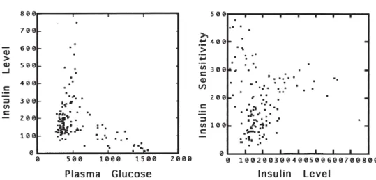
Figure 1 displays the bivariate scattergrams of the original values of glyce-mia by insulin output and of insulin output by insulin sensitivity for the 145 patients. Only these two relationships are taken up here. Figure 2 displays the same bivariate relationships according to the logs of the observations. The three clinical groups of subjects appear well surrounded by 95% equiprobable ellipses, thereby suggesting bivariate lognormality. The good fit sug-gests that the fractal model can describe glucose disposal in all three clinical groups of subjects. Ellipse major axes are also drawn in Figure 2; the major axes are the power laws of the first PCA (to be presented below). In order not to clutter Figure 2, the power laws of the second PCA (perpendicu-lar to the major axes) have not been sketched out.
Tables 1, 2, and 3 set out PCA results. Table 4 displays power-law exponents. Only the first two components are shown be-cause their contribution to variability amounts to nearly the total variance. Table 1 suggests that the group of normal subjects is heterogeneous with 73% of the variance explained by the first component. This
Figure 1 - Scattergram of plasma glucose (mg/100ml/hr) by insulin concentration (µU/ml/hr):
component is dominated by insulin sensi-tivity and concentration. It shows that a glu-cose load does not elicit a high concentra-tion of plasma glucose.
Insulin concentration, however, is pro-portional to power 9 of plasma glucose (Table 4), and sensitivity increases accord-ing to power 2 of insulin concentration. To fix ideas, a proportional increase of power 1 would mean equal increase over any two variables. In the case of the glucose and in-sulin concentration of normal subjects, the result shows that a unit increase in glucose
entails a nonlinear reaction of insulin with the latter increasing as power 9 of glucose. As we shall see below, this power curve is far less steeper than that found in NIDDM subjects. Because these results pertain to presumably normal subjects, the results can be considered the gold standard against which findings on diseased subjects ought to be assessed. The first component there-fore describes how normal subjects quan-titatively dispose of a glucose load.
The second component of the normal group is dominated by the contrast of insu-lin concentration and sensitivity. Sensitiv-ity decreases very slowly according to a power of -0.5, with an increase in insulin concentration. This component of variation is not negligible (accounting for 24% of the total variance). It describes how clinically normal subjects qualitatively dispose of a glucose load. The inverse power law indi-cates that this is a source of pathological variation.
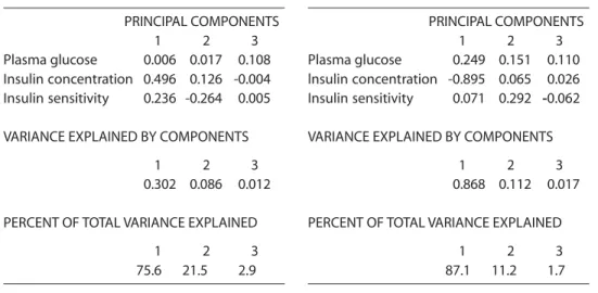
The results of the analysis of the data obtained from the subjects diagnosed with NIDDM are presented in Table 2. The analy-ses shown in Table 4 indicate that, in these subjects, glucose disposal (first component) required very high concentrations of insu-lin (ß=82.7) and that sensitivity is low
Table 1 - PCA component loadings in
clinically normal subjects.
PRINCIPAL COMPONENTS
1 2 3
Plasma glucose 0.026 0.008 -0.103 lnsulin concentration 0.239 0.281 0.005 lnsulin sensitivity 0.496 -0.136 0.003
VARIANCE EXPLAINED BY COMPONENTS
1 2 3
0.304 0.098 0.011
PERCENT OF TOTAL VARIANCE EXPLAINED
1 2 3
73.6 23.7 2.7 Figure 2 - Scattergram of plasma glucose
(mg/100ml/hr) by insulin concentration (µU/
(ß=0.5) in comparison with normal subjects (Table 1 first component). On the other hand, accounting for 21% of the variance, the second component indicates an impor-tant decrease in sensitivity (ß=-2.1) with low insulin output. The second component points to a source of pathological variation similar to but more severe than of the clini-cally normal subjects (Table 1 second com-ponent).
The results of the analysis of the data
obtained from the subjects diagnosed with IDDM are presented in Table 3. This group is more homogeneous, where the first com-ponent accounts for 87% of the total varia-tion. The analysis shown in Table 4 suggests an abrupt decrease in insulin output when plasma glucose concentration was high (Table 3). The second component, which represents a low source of total variation (11%), shows low insulin output but very high sensitivity to insulin.
Table 2 - PCA component loadings in clinically diagnosed NIDDM subjects.
PRINCIPAL COMPONENTS
1 2 3
Plasma glucose 0.006 0.017 0.108 Insulin concentration 0.496 0.126 -0.004 Insulin sensitivity 0.236 -0.264 0.005
VARIANCE EXPLAINED BY COMPONENTS
1 2 3
0.302 0.086 0.012
PERCENT OF TOTAL VARIANCE EXPLAINED
1 2 3
75.6 21.5 2.9
Table 3 - PCA component loadings in clinicaliy diagnosed IDDM subjects.
PRINCIPAL COMPONENTS
1 2 3
Plasma glucose 0.249 0.151 0.110 lnsulin concentration -0.895 0.065 0.026 Insulin sensitivity 0.071 0.292 -0.062
VARIANCE EXPLAINED BY COMPONENTS
1 2 3
0.868 0.112 0.017
PERCENT OF TOTAL VARIANCE EXPLAINED
1 2 3
87.1 11.2 1.7
Table 4 - Power law exponents estimated over the first two principal components.
Clinically normal subjects
lnsulin =* Sensitivityb** Glucose = lnsulinb
First component 2.1 9.2
Second component -0.5 35.1
Clinically diagnosed NIDDM subjects
lnsulin = Sensitivityb Giucose = lnsulinb
First component 0.5 82.7
Second component -2.1 7.4
Clinicaliy diagnosed IDDM subjects
lnsulin = Sensitivityb Glucose = Insulinb
First component -0.08 -3.5
Second component 4.5 0.4
Discussion
The methodology used in this paper is not new. The allometry law is often found in biology. PCA is ubiquitous in science, and fractals are common in physics. What is new is the unification of fractal modeling, allo-metric law, and the principal components in the framework of a coherent methodol-ogy intended to understand the nonlinear dynamics (by FCAS) of diabetes.
These analyses suggest that glucose dis-posal can be considered a FCAS. This con-clusion is supported in normal, NIDDM, and IDDM subjects. The conclusion is based on a good log-log fit of the three bio-logical variables (plasma glucose, insulin concentration, and insulin efficiency) to a power law. Identifying a system as FCAS leads to invoking a fractal process in diabe-tes, i.e., to stating that glucose management is controlled by amplification12. This
state-ment means that there must be secondary mechanisms of glucose disposal besides insulin. These mechanisms are leverage mechanisms. Leverage can be understood in the following way. Suppose one wishes to work more efficiently. What is this per-son expected to do? He/she has two choices. First, work more, i.e., work during the eve-nings, the week-ends, etc. Such a regimen eventually leads to exhaustion. If over-whelmed by work, the person also has a sec-ond choice, i.e., hire a team that will work “under” him/her and according to his/her needs. This is a leverage mechanism. Fur-ther, nothing prevents the team members from sharing the work with others, hired on an irregular basis. Amplification, a charac-teristic of fractal processes, has the virtue of fine-tuning complex processes that need constant and subtle adjusting to challenging environmental conditions11,12. Studies on
diabetes confirm the presence of more than one mechanism of glucose disposal in hu-mans25. There are redundant glucoregulatory
factors, and a hierarchy exists among them. Although insulin stands at the top of the hi-erarchy, glucoregulation is not achieved by insulin alone.
The use of PCA has identified two inde-pendent components of variation in each clinical group. One component is associ-ated with quantitative glucose disposal and the other with insulin efficiency. Subjects with IDDM had large loadings on the first component, and those with NIDDM corre-lated strongly with the second component. According to this distinction, IDDM is clearly different from NIDDM. Whereas IDDM is a defect of insulin output, NIDDM is a defect of insulin efficiency. It was in-triguing to observe that normal subjects also loaded lightly on the second component.
The use of PCA also resulted in the iden-tification of distinct pathological processes within clinical groups, thereby reflecting the involution of the covariance structure. Co-variance structure involution was observed when the power-law exponent turned from a positive to a negative value. This change is based on the assumption that healthy bio-logical processing implies positive relation-ships among variables. This statement is true for glucose disposal. Other biological processes might behave differently.
mimic the intrinsic complexity of the glu-cose handling process of normal subjects, a much smoother intervention would be required. As a result, current insulin therapy is only expected to crudely control hyperg-lycemia. Besides, the insulin-sensitivity-to-production ratio has a nearly null exponent (-.08). The latter exponent suggests that in-sulin sensitivity is left uncontrolled in IDDM patients. The latter conclusion would be consistent with a basic pleiotropic defect.
The NIDDM clinical group also supports the quantitative-glucose-disposal interpre-tation of the first principal component. This finding suggests that NIDDM patients have hyperinsulinemia following a glucose load. The most popular interpretation of this re-lates to lower than normal insulin sensitiv-ity, i.e., insulin resistance. This hypothesis is not contradicted by the results. A com-peting hypothesis would be that hyper-insulinemia leads to low efficiency; this can occur if insulin becomes insensitive after a threshold level of insulin secretion is ex-ceeded. A first mechanism explaining the latter hypothesis might be a defect in insu-lin structure; a second mechanism would be impaired insulin bioreactivity. The lat-ter hypothesis is in line with the IDDM sec-ond component according to which very low insulin output accompanies very high insulin sensitivity.
The second principal component relates to insulin efficiency. Definite insulin resis-tance is noted in the clinically normal and NIDDM groups. The sensitivity problem is not dramatic in clinically normal subjects who are (and may remain) symptomless. This might refer to a subtle aging effect. The exponent of -0.5 points to a highly complex mechanisms of glucose regulation. This ex-ponent also implies that the insulin insen-sitivity of the normal subjects is due to com-plex interactions among several finely-tuned mechanisms.
Insulin sensitivity is definitely impaired in the NIDDM clinical group. The defect is more severe than that of normal subjects. The defect, with a powerlaw exponent of -2.1 is crude, and can be located deep in the
hierarchy of insulin-sensitivity control achievement. It suggests a well-delineated clinical picture consistent with a potent ge-netic initial condition that can bypass the complex dynamics’ nonlinearities of the pathological process. More often than not complex nonlinearities will prevent any eas-ily-recognized one-to-one relationship be-tween cause and effect in disease processes. Further, the small exponent suggests a per-sistence effect, i.e., lack of control due to poorly scheduled feedbacks. Such a high exponent is in contradistinction with the swift response of normal subjects to a glu-cose challenge. The persistence effect might therefore coincide with a lower-than-nor-mal peripheral sensitivity to insulin. This explanation is in line with a post-receptor defect in peripheral tissues and hence with poor negative insulin feedback26.
The NIDDM persistence effect is quite crude, thus preventing any capacity of com-plex and finely-tuned regulation. Further, insulin efficiency proved to be lower-than-optimal in normal subjects; this suggests a lengthy pre-diabetic process to the NIDDM clinical state. This suggestion is not at vari-ance with a genetic hypothesis but never-theless more in line with a long-run (con-tinuous) environmental and/or behavioral effect. The reducing of physical activity with age is a likely intervening event. The latter considerations mean that normal glucose regulation is controlled by swift reaction times due to fine-tuning by the glucose-regulation control hierarchy. The latter con-trol is lost in NIDDM. All the above results are consistent with the most recent research results on diabetes26, 27.
second component would represent undiag-nosed but precocious cases of NIDDM. This pre-diabetic condition would evolve to a full-blown NIDDM dynamical process as exemplified by the NIDDM group second-principal-component. Similarly, the first component of the NIDDM group would de-scribe subjects having a normal response to a glucose load, i.e., simple hyperinsulinemia with lower yet normal insulin sensitivity. These subjects would incorrectly be consid-ered NIDDM patients. Likewise, the clinical IDDM group would be composed of two sub-groups. The first component would point to the most common IDDM type with auto-immune insulin destruction. The second component would refer to subjects with un-usually high glucose concentrations, very low insulin output, but very high insulin ef-ficiency. These normal subjects would pre-sumably be those with incipient beta-cell de-struction28.
This epidemiologic study of a complex disease is the first to make use of FCAS mod-eling. For a first study, methodological and interpretative aspects have been empha-sized. Further, to test the new methodology, the analysis has been carried out on a com-plex but well-studied disease process. Cross-sectional data such as those used here are easy to gather and they can yield important clues as to the disease process. Purely dynamical data allowing for multiple repeated measurements would nonetheless be the most useful approach in unravelling the various steps of the pathological pro-gression. Though this cross-sectional analy-sis cannot definitely distinguish between a disease’s natural history and subgroups’ heterogeneity, it is surmised that this type of data reveals a dynamic viewpoint, for the power law describes how biologic variables change in different subjects. Our results are in line with what is known of the biology of diabetes, and agrees well with past appli-cations of the method to other complex bio-logical processes. This gives credence to the validity of the methodology used. The FCAS model can assess the complexity of a dis-ease process. FCAS does not evaluate
cau-sality. In no way the computed the power-law exponents (or FDs to be calculated therefrom) are indices or arguments on be-half of causality. To be specific, FCAS pro-vides an assessment of the complexity of the dynamics of the process. Furthermore, this study suggests new directions of research. Future diabetes studies using fractal mod-eling ought to be undertaken with biologi-cal components (e.g., glucagon) reflecting various scales in the hierarchy of glucose handling. It would also be important to carry out this type of analysis on less known but equally complex disease processes. The results could uncover unusual findings and provide clues to further research.
Acknowledgements
We are particularly indebted to Nick Birkitt, Michael J. Glade, Elizabeth Lin, Will Maier, and Dena Schanzer for many help-ful comments and suggestions. We are also grateful to Katherine Frohlich and Ron Levy for a review of the manuscript style.
APPENDIX I
CONCEPTUAL UNDERPINNINGS OF CONCEPTUAL UNDERPINNINGS OFCONCEPTUAL UNDERPINNINGS OF CONCEPTUAL UNDERPINNINGS OFCONCEPTUAL UNDERPINNINGS OF FCAS
FCASFCAS FCASFCAS
FCAS, when applied to health and dis-ease, proposes to replace the concept of states with that of processes. Second, the approach considers disease as an emergent property resulting from a late, abrupt, and unsuccessful attempt of the organism to maintain homeostasis16. In the context of
FCAS, precisely because complex diseases imply emerging behaviors, “homeo-dynamics” is a more appropriate term than homeostasis30. The latest property of the
mol-ecules self-organized into ice crystals) in-duced by far-from-equilibrium dynamics, with irreversibility as the endpoint17.
Dis-equilibrium is conceived as a dynamic state which includes the seeking of solutions to environmental aggression. This definition of disease further implies that the patho-logical process cannot be considered sepa-rate from the health process18. One
there-fore has to model health and disease pro-cesses together. A remarkable expository paper of possible FCAS in hypertension is Weder & Schork19.
Considering health and disease as a complex dynamic has two important con-sequences. First, clinical disease is the lat-est of the emergent properties of the gradual dynamic unfolding of the subject’s historical events. This memory-keeping but incessantly reorganizing complex structure is based on interrelated events. Second, in-puts to this process are shared by several different interacting scales of biological or-ganization involving feedback. The overall result of this complex parallel processing is information translation and specificity loss. Therefore, any clinically observable prop-erty is a process endpoint whose causes cannot be linearly determined. A possible metaphor for the pathological process is a walk in a maze, the walls of which rearrange themselves with every step20.
APPENDIX II
MATHEMATICAL UNDERPINNINGS OF MATHEMATICAL UNDERPINNINGS OF MATHEMATICAL UNDERPINNINGS OF MATHEMATICAL UNDERPINNINGS OF MATHEMATICAL UNDERPINNINGS OF FRACTAL MODELING
FRACTAL MODELING FRACTAL MODELING FRACTAL MODELING FRACTAL MODELING
The inverse power law is a hyperbolic function with no characteristic scale and, therefore, infinite moments. In particular, its theoretically infinite variance provides space over all scales of organization for un-expected emergent events. The positive power law is given by: Y = a X ß where a is a
parameter, X and Y are two intercorrelated biological variables, and ß is the power-law exponent. In biology, this equation is known as the allometric law21. The exponent of the
power law is usually positive. It describes
the differential rate of change of two vari-ables from a cross-sectional survey of or-ganisms. When fitted to the bivariate rela-tionship of variables on log-log graph pa-per, the function yields a straight line.
A covariance structure refers to a set of multiple interrelated variables. To deal with multiple variables does not detract from using the power law. Incidentally, the fit-ting procedure through the major axes gen-eralizes easily to multiple variables through principal component analysis (PCA)22.
The power-law exponent can be esti-mated in many ways. In physics, it is usu-ally estimated by least squares15. This poses
a unique problem for biological variables since no dependent variable is implied by the concept of covariance structure. Fur-ther, the X and Y variables both involve measurement errors. The best way to deal with this situation is to estimate the slope of the major axis (instead of any of the re-gression lines). Accordingly, neither the X nor the Y variable should be privileged by the fitting procedure: the minimization should then be undertaken orthogonally with respect to the major axis instead of vertically or horizontally with respect to re-gression lines. Doing so, however, involves one further difficulty: the slope of the ma-jor axis is attracted towards the variable with the largest measurement error or the largest scale. One then has to take the loga-rithm of the variables to stabilize the vari-ance or render the slope estimate scale-in-variant under nonlinear scale changes22,29.
Seeking the principal components of the covariance matrix of the log variables of a bivariate swarm of points yields a matrix of loadings, the first vector of which represents the direction cosines of the major axis and the second vector, the direction cosines of the minor axis such that:
Y1 = [cos t sin t] [X1 - µ1]
Y2 = [-sin t cos t] [X2 - µ2]
are the direction cosines of the rotation to the new axes, and the [Xi - µi] correspond to the translation with respect to the original coordinate axes undertaken by the PCA. The µi are the means of the original Xi variables. The above yields:
{Y/Gy} 1/cos t = {X/Gx} 1/sin t
where: Y and X are the arithmetic values; Gy and Gx are the geometric means of Y and X;
and cos t and sin t are the direc-tion cosines of the matrix of factor loadings of the logarithmic covari-ance matrix.
It results from the above that:
Y = {Gy/Gx(cos t/sin t)} X(cos t/sin t)
and therefrom: Y = a X ß
Therefore, the above transforms back to the power law, yielding the exponent ß as the ratio of the direction cosines of the
bi-variate swarm of points. Compared to esti-mating through least squares, there are three advantages to the above procedure. First, the slope of the power law is biologi-cally meaningful because it specifies a structure rather than a dependence rela-tionship. Second, one obtains not only the value of the slope but also the estimates of differential change in both variables. Third, one can straightforwardly assess the com-plexity of the dynamics from a simple as-sessment of the power-law exponent.
Obtaining the slopes of the orthogonal axes of a high-dimensional swarm of points is a simple matter of performing a PCA on the covariance matrix of the logged data. More specifically, the matrix of factor load-ings then yields the direction cosines of all the axes of the hyperellipsoid. The direction cosines can then be used to estimate the various power-law slopes. To use principal components on the logged data of the co-variance matrix, one must ensure that the swarm of points is normally distributed; this can be assessed by a 95% equiprobable el-lipse contour on each pair of variables29.
References
1. Krieger N. Epidemiology and the web of causation: Has anyone seen the spider? Soc Sci Med 1994; 39: 887-903.
2. Halloran ME, Struchiner CJ. Study designs for dependent happenings. Epidemiology 1991; 2: 331-8.
3. Koopman JS, Longini Jr, IM. The ecological effects of individual exposures and nonlinear disease dynamics in populations. Am J Publ Health 1994; 84: 836-42.
4. Philippe P. Chaos, population biology, and epidemio-logy. Some research implications. Hum Biol 1993; 65: 525-46.
5. Horwitz RI, Feinstein AR. Methodologic standards and contradictory results in FCASe-control research. Am J Med 1979; 66: 556-84.
6. Feinstein AR. Scientific standards in epidemiologic studies of the menace of daily life. Science 1988; 242: 1257-63.
7. Taubes G. Epidemiology faces its limits. Science 1995; 269: 164-9
8. Philippe P. Sartwell’s incubation period model revisited in the light of dynamic modeling. J Clin Epidemiol 1994; 47: 419-33.
9. May RM. Nonlinearities and complex behavior in simple ecological and epidemiological models. Ann NY Acad Sci 1987; 504: 1-15.
10. Baxt WG. Complexity, chaos and human physiology: The justification for non-linear neural computational analysis. Cancer Lett 1994; 77: 85-93.
11. Montroll EW, Shlesinger MF. On 1/f noise and other distributions with long tails. Proc Natl Acad Sci USA 1982; 79: 3380-3.
12. West BJ, Shlesinger MF. The noise in natural phenomena. Am Sci 1990; 78: 40-5.
13. Bak P, Chen K. Self-organized criticality. Sci Am 1991 Jan; 264: 46-53.
15. West JB, Deering WD. The lure of modern science: Fractal thinking. World Scientific Publishing; 1995.
16. Sing CF, Zerba KE, Reilly SL. Traversing the biological complexity in the hierarchy between genome and CAD (coronary artery disease) endpoints in the population at large. Clin Genet 1994; 6: 6-14.
17. Yates FE. Order and complexity in dynamical systems. Homeodynamics as a generalized mechanisms for biology. Math Comput Modelling 1994; 19: 49-74.
18. Firth WJ. Chaos —predicting the unpredictable. Br Med J 1991; 303: 1565-8.
19. Weder AB, Schork NJ. Adaptation, allometry, and hypertension. Hypertension 1994; 24: 145-56.
20. Baum F. Researching public health: Behind the qualitative-quantitative methodological debate. Soc Sci Med 1995; 40: 459-68.
21. Sernetz M, Gelleri B, Hofmann J. The organism as bioreactor. Interpretation of the reduction law of metabolism in terms of heterogeneous catalysis and fractal structure. J Theoret Biol 1985; 117: 209-30.
22. Jolicoeur P. The multivariate generalization of the allometry equation. Biometrics 1963; 19: 497-9.
23. Reaven GM, Miller RG. An attempt to define the nature of chemical diabetes using a multidimensional analysis. Diabetologia 1979; 16: 17-24.
24. Andrews DF, Herzberg AM. Data. A collection of problems from many fields for the student and research worker. New York: Springer-Verlag; 1985.
25. Cryer PE. Regulation of glucose metabolism in man. J Intern Med Supplement 1991;735: 31-9
26. Yki-Jarvinen M. Pathogenesis of non-insulin-dependent diabetes mellitus. Lancet 1994; 343: 91-4.
27. Stout RW. Glucose tolerance and ageing. J R Soc Med 1994; 87: 608-9.
28. Ciampi A, Schiffrin A, Thiffault J, Quintal H, Weitzner G, Poussier P, Lalla D. Cluster analysis of an insulino-dependent diabetic cohort towards the definition of clinical subtypes. J Clin Epidemiol 1990; 43: 701-15.
29. Jolicoeur P, Heusner A. The allometry equation in the analysis of the standard oxygen consumption and body weight. Biometrics 1971; 27: 841-55.