INTRODUCTION
One of the most useful techniques in plant breed-ing is the analysis of diallel crosses, which is a scheme of crosses where each individual is crossed with the remain-ing individuals. These crosses result in two types of off-spring, half and full sibs. Therefore, the breeder can infer the predominant type of gene action, additive or non-addi-tive, and select the parents for an intra- or interpopulational breeding program.
Sprague and Tatum (1942) called the additive por-tion of genotypic variance “general combining ability” (GCA), determined by mean hybrid performance of a de-termined line. The non-additive portion was the “specific combining ability” (SCA), a measure for cases where some hybrid combinations are better, or worse, than expected based on mean performance of the lines evaluated.
Among the methods available for diallel analysis, Griffing’s method 2 (1956) for the diallel formed by p pa-rental and their p(p-1)/2 F1’s, totaling n = p(p+1)/2 treat-ments considered of fixed line effects (model 1), has been one of the most frequently used. The statistical model is:
Yij = m + gi + gj + sij + εij. (i)
where,
Yij = mean value of parental (i = j) or hybrid combination (i ≠ j) with i and j = 1, 2, . . . , p;
m = general mean;
gi, gj = GCA effects of i-th and j-th parent;
sij = SCA effect of the cross among the i-th and j-th par-ents, with sij = sji;
εij. = mean experimental error.
However, the selection of parents based on a single environment may lead to unsatisfactory results for farm-ers who are in a region different from that where the culti-var was developed, due to genotype x environment inter-action effects.
When a diallel is performed in a series of environ-ments, the genotype x environment evaluation of effects in phenotypic characteristics is possible. In this situation, the model (i) becomes:
Yijk = mk + gik + gjk + sijk + εijk. (ii)
where the subscript k refers to the k-th environment where the diallel is performed.
The method of Eberhart and Russell (1966) used to study the genotype x environment interaction and the phenotypic adaptability and stability, based on simple re-gression analysis, is also widely used because of its sim-plicity and efficiency, as shown by several authors work-ing with various crops (Oliveira, 1976; Gama and Hallauer, 1980; Miranda, 1993; Gonçalves, 1997; Vendruscolo, 1997). The model, considering data from one diallel, is:
Yijk = β0ij + β1ij Xk + δijk + εijk. (iii)
where,
Yijk = the dependent variable, which refers to the genotype observation originated by crossing i-th and j-th parents in the k-th environment;
Xk = the independent variable, referring to the k-th envi-ronmental value.
It can be demonstrated that: METHODOLOGY
ASSOCIATION BETWEEN GRIFFING’S DIALLEL AND THE ADAPTABILITY AND
STABILITY ANALYSES OF EBERHART AND RUSSELL*
Cleso Antônio Patto Pacheco1, Cosme Damião Cruz2 and Manoel Xavier dos Santos3
A
BSTRACTThe objective of the present work was to provide a meth-odology to study the inheritance of adaptability and stability through the breakdown of Eberhart and Russell regression coefficients and regression deviations in effects due to the mean and additive genetic effects (gi’s and gj’s) as well as dominance effects (sij’s) of Griffing´s methodology, when the diallel is conducted in several environments. It was concluded that the adaptability and stability parameters are determined in the same manner as are genetic effects. So an F1 cross inherits half the general combining ability (GCA) mean effect from each parent, while the effects due to specific combining ability (SCA) are subjected to the same con-siderations relative to sij’s, i.e., they are dependent on specific com-binations.
*Part of a thesis presented by C.A.P.P. to the Universidade Federal de Viçosa, Viçosa, MG, in partial fulfillment of the requirements for the Doctoral degree.
1Embrapa/CNPMS, Caixa Postal 151, 35701-970 Sete Lagoas, MG, Brasil.
Send correspondence to C.A.P.P. E-mail: [email protected]
2Universidade Federal de Viçosa, DBG, 36570-000 Viçosa, MG, Brasil.
∑ = β − ∑
= =
β a a
1 k Xk ij 1 a a
1 k Yijk ij
where,
β1ij = the linear regression coefficient, a relationship of the covariance of the dependent variable with the indepen-dent variable and the variance of the environment values; when the magnitude of β1ij is higher, lower or equal to 1.0 a treatment can be considered as favorably, unfavorably or generally adapted to environments, respectively; β0ij = the intercept or the point where the straight line crosses the Y axis;
δijk = the deviation of regression; εijk. = the mean experimental error.
Eberhart and Russell (1966) proposed the use of regression deviation to measure production stability. If the regression deviations are null, the cultivar has a predict-able behavior. As it is not possible to know the real envi-ronmental value, this methodology adopts an environmen-tal index (Ik), estimated for each environment by the fol-lowing expression:
where the Xk term is represented by the mean, in the k-th envi-ronment, of the evaluated genotypes, or , where possible genotypes, evaluated by method 2, model 1, in the diallel analysis from Griffing (1956).
On the other hand, a gap in quantitative genetics about the genetic control of adaptability and stability ex-ists. A relatively large number of papers reporte that the factors which determine adaptability and stability are ge-netically controlled (Gama and Hallauer, 1980; Torres, 1988; Vencovsky and Barriga, 1992). However, evidence such as that of Torres (1988), that genetic control of adapt-ability is independent of yield, is scarce and does not ex-plain how these parameters are inherited.
Recently, several authors (Naspolini Filho et al., 1981; Gama et al., 1984; Lopes et al., 1985; Eleutério et al., 1988, Parentoni et al., 1990, Santos et al., 1994 and Pérez-Velásquez et al., 1995), concerned with genotype x environment interaction in their breeding programs, have used the diallel under different environmental conditions. However, their methodology does not allow study of the adaptability of the estimated genetic effects. They had to
restrict themselves to detecting the existence of interac-tion of these effects with the environments and recommend-ing their materials based on the mean effects, accordrecommend-ing to the wide adaptability of these materials.
This study was carried out to develop a methodol-ogy for inheritance studies of adaptability and stability of production by an association of diallel analysis methodol-ogy (Griffing, 1956) with adaptability and stability analy-sis (Eberhart and Russell, 1966). The proposed methodol-ogy was then used in a diallel cross among maize popula-tions assessed in a number of environments.
MATERIAL AND METHODS
Applying the two mathematical models described in the introduction ((ii) and (iii)) for data obtained from replicated diallels from several environments, it can be seen that although they lead to completely different results they originated from the same phenotypic observationYijk, where the indices i and j refer to parents involved in the diallel cross and the index k refers to the environment where the diallel was carried out. Then, considering that the Eberhart and Russell (1966) model is based on simple linear re-gression and, further, that the genetic effects estimated by method 2, model 1, by Griffing (1956) are additive, a new model may result from the association of the two previous:
Yijk = mk + gik + gjk + sijk + εijk =
= β0ij + β1ij Ik + δijk + εijk. (iv)
It may be used by focusing on multiple linear regression. Assuming one diallel with p parents (i = j = 1,. . ., p) and its p(p -1)/2 F1 crosses, assessed in a environments (k = 1, . . .,a), and using matrix form, the model (iv) be-comes Y = Xβ + ρ for each ij, where Y is a matrix (a x 4) of the genetic effects estimated by Griffing’s methodol-ogy, relative to the ij genotype in several environments; X is an (a x 2) matrix where 2 is the number of parameters to be estimated; β is a (2 x 4) matrix whose elements are established by partitioning the parameters to be estimated; and ρ is an (a x 4) error matrix. Thus:
=
Ia 1
I 2 1
I1 1
X
L L
∑ = −
= a a
1 k Xk Xk
Ik
n n
j i Yijk X k ∑
≤ =
2 ) 1 p ( p
n = +
= =
sija g ja gia ma
s 2ij g 2j g 2i m2
s 1ij g 1j g 1i m1
Yija Y 2ij Y 1ij
Y
L L L L L
;
; ∑
= − ∑=
∑
= − ∑= ∑=
= β
a
1 k
a 2 a
1 k Xk X2k
a 1 k
a a
1 k Xk a
1 k Yijk X
Yijk k ij
1
The matrices for the sum of squares (SS) of sev-eral environments with the same genotype (SSA/G), the regression (SSReg) and the regression deviations (SSDev) are also obtained by the least squares method. The sim-plest way to express the decomposition of regression de-viations due to genetic effects from Griffing’s model was by relationship between the deviation means squares (MSD) of the regression with the residual mean squares (MSR), as an F-test decomposition:
However, the decomposition parts do not associ-ate with any probabilistic function.
Yield data (kg/ha) from 28 maize populations and their 378 diallel crosses assessed in 10 environments (Pacheco, 1997) were used as an example.
RESULTS AND DISCUSSION
Diallel crosses in each environment and pooled together gave significant values for GCA and SCA effects
and their interaction with the environments. The GCA/ SCA ratio (0.871) showed that the effects of the devia-tions due to dominance predominated over the additive.
The proposed methodology allows the study of the adaptability and stability of the genetic effects estimated by Griffing’s (1956) methodology, using a partitioning of Eberhart and Russell’s (1966) parameters and observations from the diallel experiments carried out in several envi-ronments; however, the interpretation of the results should be made using both methodologies.
The data from six populations are shown as an il-lustration.
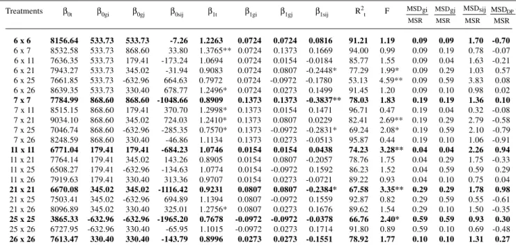
There are seven more columns in Table I than would be expected by simply joining the two methodologies; three refer to the partitioning of the total regression coefficient (β1t), and the other four express the deviation from the re-gression of the genetic effects compared with the mean square of the residual.
When the data (Table I) are analyzed, the most important point is that the adaptability and stability pa-rameters are subjected to the same rules that govern the inheritance of quantitative traits. Therefore, in the absence of dominance and epistatic effects, as an F1 cross inherits half the additive effects from each parent, the behavior of the sibs would be completely predictable from the par-ents’ behavior. If it were not for the effects of specific com-bination, the ideal cross could be predicted among the two
ε + δ ε + δ ε + δ ε + δ ε + δ ε + δ ε + δ ε + δ ε + δ ε + δ ε + δ ε + δ = ρ
s aij
sija g ja g ja gia gia mija mija
s 2ij
s 2ij
g 2j
g 2j
g 2i
g 2i
m 2ij
m 2ij
s 1ij
s 1ij
g 1j g 1j
g 1i
g 1i
m 1ij
m 1ij
L L
L L
The β matrix is estimated by the normal equation system in the following way: β = (X’X)-1X’Y
where, ^ ∑ = ∑ = ∑ = ∑ = ∑ = ∑ = ∑ = ∑ = ∑ = ∑ = ∑ = ∑ = = β a 1 k
I 2k I k a 1 k sijk a 1 k
I 2k I k
a 1 k g jk a
1 k
I 2k I k a 1 k gik a 1 k
I 2k a
1 k
I 2k
a a 1 k sijk a a 1 k g jk a a 1 k gik a a 1 k mk ˆ β β = β β = β t 1 t 0 ij 1 ij 0 β β β β β β β β 1sij 1gj 0sij 0gj 0m gi 1 m 1 gi 0
= , and
parents which had at the same time the highest gi’s and the lowest β1gi’s and regression deviations.
A negative β1sii means that as the environmental effects increased, the sii parameter decreased. In this case, however, a large, negative sii is desirable because it is associated with deviation due to positive dominance. A positive β1sii is of no interest to breeders. The genetic in-terpretation of sii parameter (the SCA of parent i with it-self) was given by Cruz and Vencovsky (1989). They showed that this parameter is indicative for unidirectional dominance and for varietal heterosis, being represented by the magnitude of the analysis and through the sii esti-mated signs. Therefore, negative values of sii are associ-ated with positive deviations due to dominance and the magnitude value is indicative of the varietal heterosis or indicative of the population genetic divergence in rela-tion to the diallel mean. It was demonstrated by Cruz and Vencovsky (1989) that the summation of the sii is a linear function of the mean heterosis.
The deviations due to dominance were responsible for the slight tendency, β1t = 0.89, of BR-106 to adapt to unfavorable environments (Table I).
The BR-105 variety had an sii mean of -7.26, which leaves it with one of the lowest genetic divergences com-pared with the other assessed populations. This low ge-netic divergence means low positive deviations due to dominance, since only the CMS-15 population presented
an sii positive mean of 299.00 and was, therefore, the only one with deviation due to negative dominance.
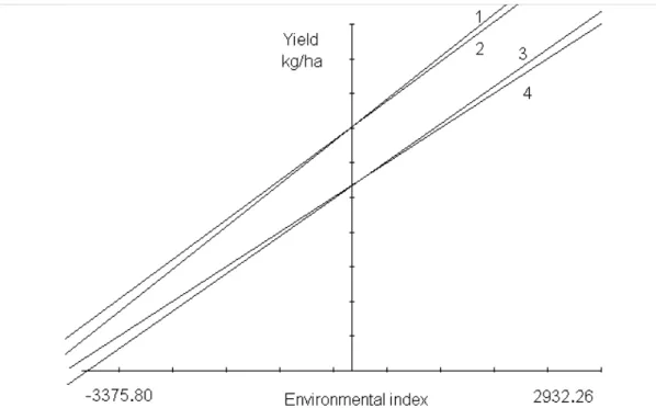
The partitioning of β1t for BR-105 showed that its sii’s increased (became less negative) in the same direction as the environmental effects, indicating that its deviation due to dominance decreased from the worst to the best environ-ment, in an inverse behavior to that found for BR-106 (Fig-ures 1 and 2). The effect of the genetic parameters in the slope of the straight line, considering the full model (m + 2gi + sii) proposed by Griffing (1956), can be better understood when compared with the representative lines of the partial models, separately considering the effects of the GCA (m + 2gi) and SCA (m + sii), lines 2 and 3, respectively.
The negative or positive slopes can be determined by comparing the angles formed between the X axis (en-vironmental indices) and the first three lines with the angle formed between line 4 and the X axis, that represents the regression of the general means (m) with the environmen-tal indices. This genetic parameter will be positive when the slope of the straight line becomes greater than the straight line 4, or negative when the slope becomes shorter. The magnitudes from the effects of the GCA and SCA give an idea of the contribution of the additive and non-additive effects to the adaptability of the material evaluated, while the positive or negative signs showed if the effects increased or decreased in the same direction as the environmental variation stimulus.
Table I - Adaptability and stability parameters from Eberhart and Russell (1966) and their partitioning by the effects of Griffing’s (1956) general and specific combining effects. Sampling of a diallel among 28 populations and their 378 F1s, assessed in 10 environments.
Treatments β0t β0gi β0gj β0sij β1t β1gi β1gj β1sij R2t F
6 x 61 8156.64 533.73 533.73 -7.26 1.2263 0.0724 0.0724 0.0816 91.21 1.19 0.09 0.09 1.70 -0.70 6 x 71 8532.58 533.73 868.60 33.80 1.3765** 0.0724 0.1373 0.1669 94.00 0.99 0.09 0.19 0.78 -0.07 6 x 11 7636.35 533.73 179.41 -173.24 1.0694 0.0724 0.0154 -0.0184 85.77 1.55 0.09 0.04 1.63 -0.21 6 x 21 7943.27 533.73 345.02 -31.94 0.9083 0.0724 0.0807 -0.2448* 77.29 1.99* 0.09 0.29 1.03 0.57 6 x 25 7661.85 533.73 -632.96 664.63 0.7972 0.0724 -0.0972 -0.1780 53.13 4.59** 0.09 0.59 3.83 0.08 6 x 26 8639.35 533.73 330.40 678.77 1.2496* 0.0724 0.0273 0.1499 91.45 1.20 0.09 0.10 0.98 0.02 7 x 71 7784.99 868.60 868.60 -1048.66 0.8909 0.1373 0.1373 -0.3837** 78.03 1.83 0.19 0.19 1.36 0.10 7 x 11 8515.15 868.60 179.41 370.70 1.2998* 0.1373 0.0154 0.1471 96.71 0.47 0.19 0.04 0.32 -0.08 7 x 21 9034.10 868.60 345.02 724.03 1.2410* 0.1373 0.0807 0.0229 82.41 2.69** 0.19 0.29 2.79 -0.58 7 x 25 7046.74 868.60 -632.96 -285.35 0.7570* 0.1373 -0.0972 -0.2831* 69.24 2.08* 0.19 0.59 2.10 -0.79 7 x 26 8248.59 868.60 330.40 -46.86 1.1134 0.1373 0.0273 -0.0513 95.87 0.44 0.19 0.10 1.06 -0.91 11 x 11 6771.04 179.41 179.41 -684.23 1.0746 0.0154 0.0154 0.0438 74.23 3.28** 0.04 0.04 2.26 0.94 11 x 21 7764.14 179.41 345.02 143.26 0.8905 0.0154 0.0807 -0.2057 78.76 1.75 0.04 0.29 1.75 -0.33 11 x 25 6508.27 179.41 -632.96 -134.63 1.0774 0.0154 -0.0972 0.1592 86.23 1.52 0.04 0.59 0.59 0.29 11 x 26 7919.63 179.41 330.40 313.36 0.9707 0.0154 0.0273 -0.0721 89.22 0.93 0.04 0.10 0.75 0.04 21 x 21 6670.08 345.02 345.02 -1116.42 0.9231 0.0807 0.0807 -0.2384* 67.58 3.35** 0.29 0.29 1.78 0.98 21 x 25 7503.41 345.02 -632.96 694.89 1.1394 0.0807 -0.0972 0.1559 92.87 0.82 0.29 0.59 0.55 -0.61 21 x 26 8096.89 345.02 330.40 325.01 1.2756* 0.0807 0.0273 0.1676 89.62 1.54 0.29 0.10 1.50 -0.35 25 x 25 3865.33 -632.96 -632.96 -1965.20 0.7678 -0.0972 -0.0972 -0.0378 66.76 2.40* 0.59 0.59 0.93 0.30 25 x 26 6727.95 -632.96 330.40 -65.95 1.1015 -0.0972 0.0273 0.1714 91.80 0.89 0.59 0.10 0.69 -0.48 26 x 26 7613.47 330.40 330.40 -143.79 0.8996 0.0273 0.0273 -0.1551 78.92 1.77 0.10 0.10 1.31 0.27
Grand mean (m) = 7096.45 kg/ha; β1m = 1.0; β0t; β0gi; β0gj; β0sij = general mean to the ij genotype, and its parts due to general and specific genetic effects; β1t; β1gi; β1gj; β1sij = total regression coefficient to the ij genotype, and its parts due to general and specific genetic effects; MSR = residual mean squares
(ANOVA) and MSD = deviations from regression mean squares to general and specific genetic effects and its double products (DP); * and ** indicate significance at 5% and 1% of probability by the F-test; Rt
2 = total determination coefficient. Treatments: 6 = BR - 105; 7 = BR - 106; 11 = CMS - 14C; 21
= CMS - 50; 25 = BA-III-Tusón; 26 = Saracura.
MSR MSDgi
MSR MSDsij MSR
MSDgj
MSR MSDDPDP
Figure 1 - Simple linear regression for adaptability of the BR-105 population to the 10 assessed environments. Estimate of m + 2gi + sii (straight line 1, with β1 = 1.2263), according to Eberhart and Russell (1966) and its partitioning using Griffing’s (1956) genetic effects: m + 2gi
(line 2, β1 =1.1448), m + sii (line 3, β1 = -1.0816) and m (line 4, β1 = 1.0000).
In this way, the β1t decompositions indicate, for example, that for the BR-105 x CMS-14C cross, the aver-age SCA, besides being negative (β0sij = -632.96), results from estimates that showed decreasing behavior (β1sij = -0.0184) while the environmental stimulus was increas-ing. On the other hand, the CMS-14C x BA III Tuson cross also showed a negative genetic complementation (β0sij = -134.63), but increased in the same direction as the envi-ronmental stimulus (β1sij = 0.1592).
Eberhart and Russell’s (1966) ideal genotype can now be defined as that with a high general mean due to the high gi’s effects, and further, having β1t = 1.0, due to β1gi = β1gj = β1sij. Genotypes with regression deviations equal or close to zero were not found, even considering all the treat-ments.
Observing the F-values (Table I) for the mean squares of the regression deviations as well as the decom-positions to genetic effects and double products, a strong influence was noted from the portion of the regression deviations associated with SCA.
Considering all 28 maize populations and their 378 diallel crosses (data not shown), it was observed that, al-though the regression deviations due to SCA and due to double products were the strongest factors of production instability, the combination of the small deviations of all effects was responsible for the significance in the remain-ing 45.37% of the treatments.
CONCLUSIONS
This new methodology allowed inferences on adaptability and stability of the GCA and SCA, providing an excellent alternative for presenting results of diallel analyses carried out in several environments.
Adaptability and stability parameters are subjected to the same rules which control inheritance of quantitative traits. In the absence of dominance effects, the behavior of the sibs would be completely predictable from the par-ents’ behavior. If it were not for the specific combination effects, the ideal cross could be predicted among the par-ents which joined, at the same time, the greatest gi’s and the lowest β1gi’s and regression deviations.
RESUMO
Este trabalho teve por objetivo estudar a herança da adaptabilidade e estabilidade através do desdobramento dos coeficientes de regressão e dos desvios da regressão de Eberhart e Russell em efeitos devidos à média e aos efeitos genéticos aditivos (gi’s e gj’s) e devidos à dominância (sij’s) da metodologia
de Griffing, quando um dialelo é conduzido numa série de ambientes. Concluiu-se que os parâmetros de adaptabilidade e estabilidade são determinados da mesma maneira que os efeitos
genéticos, de modo que um F1 recebe metade do efeito médio da capacidade geral de combinação (CGA) de cada um de seus pais, permanecendo as partes devidas à capacidade específica de combinação (SCA) sujeitas às mesmas considerações pertinentes aos sij’s, ou seja, são dependentes das combinações específicas
médias.
REFERENCES
Cruz, C.D. and Vencovsky, R. (1989). Comparação de alguns métodos de análise dialélica. Rev. Bras. Genét. 12: 425-438.
Eberhart, S.A. and Russell, W.A. (1966). Stability parameters for compar-ing varieties. Crop Sci.6: 36-40.
Eleutério, A., Gama, E.E.G. and Morais, A.R. (1988). Capacidade de combinação e heterose em híbridos intervarietais de milho adaptados às condições de cerrado. Pesq. Agrop. Bras.23: 247-253. Gama, E.E.G. and Hallauer, A.R. (1980). Stability of hybrids produced
from selected and unselected lines of maize. Crop Sci. 20: 623-626. Gama, E.E.G., Vianna, R.T., Naspolini Filho, V. and Magnavaca, R. (1984). Heterosis for four characters in nineteen populations of maize (Zea mays L.). Egypt. J. Genet. Cytol.13: 69-80.
Gonçalves, F.M.A. (1997). Adaptabilidade e estabilidade de cultivares de milho avaliadas em safrinha no período de 1993 a 1995. M.Sc. the-sis, UFLA, Lavras, MG.
Griffing, B.A. (1956). Concept of general and specific combining ability in relation to diallel crossing systems. Austr. J. Biol. Sci.9: 463-493. Lopes, M.A., Gama, E.E.G., Vianna, R.T. and Souza, I.R.P. (1985).
Heterose e capacidade de combinação para produção de espigas em cruzamentos dialélicos de seis variedades de milho. Pesq. Agrop. Bras. 20: 349-354.
Miranda, G.V. (1993). Comparação de métodos de avaliação da adapta-bilidade e estaadapta-bilidade de comportamento de cultivares de feijão (Phaseolus vulgaris L.). M.Sc. thesis, UFV, Viçosa, MG.
Naspolini Filho, V., Gama, E.E.G., Vianna, R.T. and Môro, J.R. (1981). General and specific combining ability for yield in a diallel cross among 18 maize populations (Zea mays L.). Rev. Bras. Genét.IV: 571-577.
Oliveira, A.C. (1976). Comparação de alguns métodos de determinação de estabilidade em plantas cultivadas. M.Sc. thesis, UNB, Brasília, DF. Pacheco, C.A.P. (1997). Associação das metodologias de análise dialélica de Griffing e de análise de adaptabilidade e de estabilidade de Eberhart e Russell. Ph.D. thesis, UFV, Viçosa, MG.
Parentoni, S.N., Santos, M.X., Magnavaca, R., Gama, E.E.G., Pacheco, C.A.P. and Lopes, M.A. (1990). Productividad y heterosis en cruzamientos dialélicos de diez poblaciones precoces de maiz. In: XIII Reunión de Maiceros de la zona Andína. Chyclaio. Peru, pp. 33-48. Pérez-Velásquez, J.C., Ceballos, H., Pandey, S. and Díaz-Amaries, C.
(1995). Analysis of diallel crosses among Colombian landraces and improved populations of maize. Crop Sci.35: 572-578.
Santos, M.X., Pacheco, C.A.P., Guimarães, P.E.O., Gama, E.E.G., Silva, A.E. and Oliveira, A.C. (1994). Diallel among twenty-eight variet-ies of maize. Rev. Bras. Genét.17: 277-282.
Sprague, G.F. and Tatum, L.A. (1942). General vs. specific combining ability in single crosses of corn. J. Am. Soc. Agron.34: 923-932. Torres, R.A.A. (1988). Estudo do controle genético da estabilidade
fenotípica de cultivares de milho (Zea mays L.). Ph.D. thesis, ESALQ-USP, Piracicaba, SP.
Vencovsky, R. and Barriga, P. (1992). Genética Biométrica no Fitomelho-ramento. SBG, Ribeirão Preto, SP, pp. 496.
Vendruscolo, E.C.G. (1997). Comparação de métodos e avaliação da adaptabilidade e estabilidade de genótipos de milho-pipoca (Zea mays
L.) na região Centro-Sul do Brasil. M.Sc. thesis, UEM, Maringá, PR.