Prediction of claim cost in general insurance

(1)

M

ASTER

MASTER

OF

ACTUARIAL

SCIENCE

M

ASTER

´

S

F

INAL

W

ORK

INTERNSHIP

REPORT

PREDICTION

OF

CLAIM

COST

IN

GENERAL

INSURANCE

CASPER

JACOB

MOERUP

S

UPERVISORS

:

W

ALTHER

N

EUHAUS

(ISEG)

A

LEX

T

ETERUKOVSKY

(I

F

P&C

I

NSURANCE

)

(2)

Master’s Final Work Master of Actuarial Science Casper Jacob Moerup

Internship Report ISEG, June 2019

2

1. Introduction

Following an internship at If P&C insurance, Industrial Product & Price, this report summarises the work and findings that was done throughout the internship.

The internship report consists of two main sections, where the first section is dedicated to the so-called Normal Year Analysis. Normal Year is an annual analysis procedure performed during the first quarter of each year. It assesses the current state of the portfolio and updates the loss models to the current portfolio. The portfolio is assessed, and losses are modelled applying the theory covered in the lectures from the Master of Actuarial Science at ISEG.

The purpose of Normal Year Analysis is to create a foundation from which the financial plan for the following year should arise.

In the first part of my internship I conducted an analysis on the Industrial Motor Portfolio on a Nordic level (Denmark, Norway, Sweden, and Finland). The first section of the current report summarises my findings and my thoughts from this process in a chronological manner.

Theory from the lectures as well as other literature was used throughout the analysis. Computations were performed in SAS Enterprise Guide™ and Excel.

The Normal Year section will touch upon areas within parameter estimation, aggregate loss models, reserving, and time series analysis.

The second section of the report analyses a model for the claim adjustment reserves (CAR). The model is described together with an assessment of its assumptions and its application purposes. The section is rounded off with a sensitivity analysis of the impact the model has on the claim adjustment reserves.

(4)

4

2. Normal Year 2020 analysis

Normal Year analysis is a procedure which is carried out on a yearly basis approximately at the end of the first quarter.

Its purpose is to assess the current state of the portfolio by considering the changes that have incurred throughout the most recent underwriting year. As the plan for the current year has already been set, the Normal Year analysis looks one year ahead and assesses how the portfolio and the claims are expected to change.

It is on the Normal Year analysis basis that the profitability actions will be decided and subsequently carried out.

A rough breakdown of the Normal Year analysis procedure can be described in the four following steps:

1) Assessment of losses and clients

This preparatory step is focussing on understanding which client/loss information should be collected from the underwriters, which will enable the actuary to build an own

opinion on the profitability of major clients and the expected changes in portfolio including gained/lost balances.

2) Alignment meeting with underwriter.

The purpose of this meeting is to collect the information outlined in step one.

3) Adjusting the initial estimates and filtering the data for outliers which might distort the statistical analysis.

4) Fitting the loss distributions.

This report will go in depth with step 1) and 4) and leave the confidential content in step 2) and 3) out of the scope.

(5)

5

Step 1 – Portfolio overview

2.1 Industrial business line.

The industrial clients in If are defined as very large commercial clients. The cut-off limit is defined by either the number of employees (+500) or turnover (>500MSEK), both of which naturally implies a greater risk exposure. These larger clients may operate locally, but their big size often implies a risk exposure abroad. For example, a company may transport goods to another country. In the case of an incident this may impact the time between the date of the incident and the reporting date since foreign actors will be involved, and procedures usually differ across country borders. In the bigger picture, this makes the tail of the industrial portfolios longer than it may be seen in a private insurance portfolio.

Another characteristic of the industrial portfolio is the diversity among clients. Some clients are relatively small whilst other clients are huge. This is not only reflected in the premium the client pays, but also in their claim generating pattern as some clients may have a very particular business nature. From an actuarial perspective this is seen as distortion, as the usual loss models often assume homogeneity in the portfolio.

Finally, the industrial business has fewer clients than a private insurance portfolio. Fewer clients implies less data which implies greater use of assumptions and portfolios which are more prone to distortion due to inhomogeneity.

2.2 The insurance portfolio.

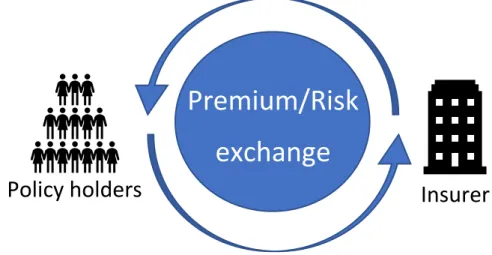
The primary inflows of the insurance company come from the clients, which in this case are the policyholders. The policyholder provides an insurance premium in exchange for a risk coverage.

(6)

6

Figure 1: Premium to risk correspondence

This is a traditional insurance portfolio. However, for the industrial business line, the left-hand side of Figure 1 is substituted with large companies (500+ employees).

Figure 2: Inhomogeneity among industrial clients

This means that the difference between policyholders is significantly larger, which is reflected in the huge variation in the insurance premium paid among industrial

policyholders. This causes some clients to have a much more distorting effect than what can be found in a traditional private insurance portfolio, where each client, in comparison, pays roughly the same premium.

For the same reason, simply building a motor insurance tariff would not work as the nature of each client’s business can vary a lot and the data provided may be too sparse to build a tariff.

Premium/Risk

exchange

Insurer

Policy holders

The size of an industrial clients can vary greatly. This is reflected in the premium the client pays, making it a suitable measure for exposure.

(7)

7

This also means that simply using a measure of exposure such as the number of policies written, will not yield a valid ratio. This is because each contribution to the “number of policies written” is equal, whereas for the “earned premium exposure” each contribution is relative to the size of the risk (and client).

One must keep in mind, however, that premiums usually do not solely reflect risk exposure. Consequently, inflation assumptions, loss/gain of clients may have a greater impact on the estimate.

It is thus crucial to carefully consider which clients’ experience represents the general underlying behaviour of the losses, and which do not.

An example can be a client with a certain business type, which makes them prone to generate a lot more claims of a particular type and size, than the average client. For

instance, a bus company driving with passengers may be a lot more prone to generate third party liability claims than another company which transport wooden benches. Those clients should not be grouped in the same portfolio which is assumed homogeneous.

2.3 Calculating earned premium.

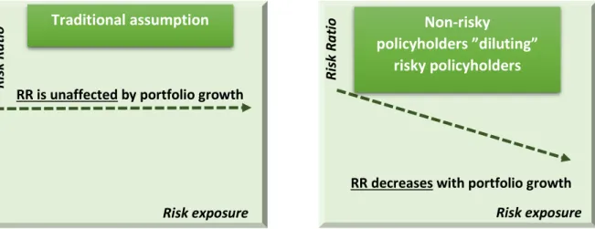
The earned premium is a figure which gets aggregated over time after a new premium has been received. As mentioned above the earned premium gives an indication to which extent the insurer is exposed to risk. In other words – larger premium means larger risk exposure. Earned premium is usually assumed to be directly proportional to the risk held. This means that the risk ratio should be unaffected by changes in the portfolio size, since a growth in risk is simply compensated by a proportional growth in the portfolio (earned premium). However, in reality we can expect differences in the risk ratio (RR = aggregate losses/earned premium) of different clients, since a lot of low risk policyholders are required to cover the losses of the high-risk policyholders (See Figure 3). This concept is known as pooling, where a lot of policyholders pay for the infrequent, large losses of few policyholders.

(8)

8

This may imply, that the risk ratio is expected to be higher for smaller portfolios and lower for larger portfolios as the pooling effect will grow stronger and finally dilute the impact from the risky policyholders.

Figure 3: Exposure impact on Risk Ratio

Figure 4: Exposure impact on Risk Ratio

One of the reasons for this is that earned premium is not an aggregation of the risk

premium (the premium that solely reflects the risk) but instead the premium the client pays, which usually contains a profit margin depending on the profitability.

In other words, the market premium (the premium paid in the market) is rarely equal to the risk premium – especially for competitive markets, where market premiums are pushed down.

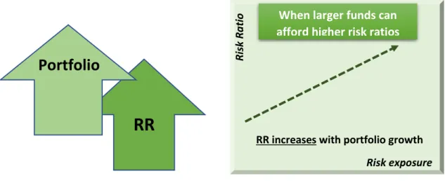
Contrasting, one could argue the opposite. As funds grow larger, larger clients could ask for lower premium while larger funds can afford higher risk ratios due to portfolio

diversification. Diversification occurs where additional losses from one client are balanced

RR

Portfolio

Risk exposure Ri sk R a ti o Traditional assumption

RR is unaffected by portfolio growth

Risk exposure Ri sk R a ti o

RR decreases with portfolio growth

Non-risky

policyholders ”diluting” risky policyholders

(9)

9

by less losses than expected from another client. Thus, with this argument the risk ratio can be expected to increase together with the portfolio.

Figure 5: Exposure impact on Risk Ratio when considering impact of larger clients pushing down premium as well as larger portfolios can afford more risk.

To summarise above reflection upon impact on the risk ratio coming from the portfolio growth, it may not be unreasonable to assume that they grow proportionally to one another since there are arguments for movements in either direction. It may in the end be a matter of the individual risk tolerance which defines how the risk ratio will behave as the portfolio grows. Some companies prefer stability and while other companies are willing to take on larger risks.

2.4 Non-correspondence between risk premium and market premium.

The portfolio analysed is a highly competitive portfolio; motor portfolio. This means that the earned premium reflects the market price rather than the actual pure risk, which by

consequence will drive up the risk ratio since a risk cover will be sold for a price lower than it should.

2.5 Assessment of ‘particular clients’.

From an underwriting perspective, no client is “bad” as long as the premium is correctly set. This view is important when assessing whether a client has distorting effect on the data as

RR

Portfolio

Risk exposure Ri sk R a ti o

RR increases with portfolio growth

When larger funds can afford higher risk ratios

(10)

10

accuracy is important, yet we do not wish to point estimate the next movement of the portfolio. Instead we wish to focus on long-term stability rather than what is going to occur tomorrow.

To quote an admirable actuary I worked with at AXA Global Life, London:

We know that we are always wrong, which is fine, if we are right on average.

Aurelie Despeyroux, Deputy Head of Reinsurance, AXA Global Re By doing so we focus on long-term stability and avoid that our estimates for the short-term future are overly biased by the most recent events.

An applicable example of this is the seasonality seen in the number of reported claims arising in a motor insurance portfolio during the winter months compared to the summer months (see Figure 5 in section 2.8). We do not want to project the behaviour of the winter months to the entire rest of the year since we can expect less reported claims in the months following the winter. Hence, by capturing this overall seasonality would give a less erratic estimate than if we simply projected the most recent movement into the near future. A “particular client” is not necessarily a client with a low profitability, but a client with a different behaviour than what could be expected from the average client.

Among these particularities a few can be mentioned as an example:

- Clients which are simply so large, that they control a large part of the portfolio - Clients with a certain business area making the client generate claims significantly

different from the expected cost per claim

E.g. a money transportation company using armed windscreen glass, which cost significantly more than a general windscreen.

Lack of data is common, and it is sometimes necessary to pick the simplest solution and add an average historical loss to represent the distorting clients’ contribution to the aggregate loss.

(11)

11

Step 4 – Fitting the loss distributions

Following an adjustment of the data such that the portfolio can be assumed homogeneous, the next step is to estimate the loss aggregate (total claim payments).

2.6 Estimating losses.

Collective Risk Theory has been used to estimate the aggregate loss of the motor portfolio for each country. The theory as well as assumptions used were taken from Klugman, Panjer and Willmot (2012).

Each risk was grouped into a subgroup describing the trigger of the loss. A few of these triggers may be:

Fire, Windscreen, Bodily injury, Property damage, and Theft.

Independence among each subgroup was assumed as well as independence among each risk. This allows for simple aggregation of the risk.

To compare the historical losses, it is important to adjust the observations for time. To do this it is necessary to make assumptions regarding the inflation. Not only a currency may devaluate over time but other factors may play a part in inflating the claim severity. It could be that salaries increase, causing the cost of windscreen replacements to go up. An intuitive choice of inflation assumption would be the consumer price index, which reflects the

historical price increases. Other, less obvious, factors to consider may be that windscreen technology gets more advanced, and thus not only the glass needs replacement but also the sensors attached to the windscreen, which make the claim severity go up. It is important that the inflation of the claims account for as many of these factors to reduce the bias of the observations.

2.7 Example: Estimating average loss per windscreen claim. We begin with defining the observations.

𝑃_𝑖,𝑡𝑊𝑖𝑛𝑑𝑠𝑐𝑟𝑒𝑒𝑛 : Each historical payment pi paid at time t given the trigger of the loss was

(12)

12

By inflating each individual historical claim to a fixed point in time (current time) we make sure all observations are comparable and representative of the losses in current time.

𝑥𝑖 = 𝐼𝑛𝑓𝑙𝑡,2019 ∗ 𝑃𝑖,𝑡𝑊𝑖𝑛𝑑𝑠𝑐𝑟𝑒𝑒𝑛. (2.1) Where,

𝐼𝑛𝑓𝑙_𝑡,2019 : inflation rate from time t up until 2019.

The collective risk model defined in Klugman, Panjer, and Willmot (2012) is of the form: 𝑆 = 𝑋₁ + 𝑋₂ + … + 𝑋_𝑁. (2.2)

Where,

S is the aggregate loss random variable, N is the total number of reported losses. We assume that when N=0 then S=0.

Since each observation is adjusted for time difference, they individually hold information about the severity of a loss occurring.

For this example, we assume that the inflation-adjusted losses, arising from windscreen damage, are described by an exponentially distributed random variable X~𝐸𝑥𝑝(𝜃), with the mean severity given by the parameter 𝜃 =1_𝜆.

We further assume that losses 𝑋𝑖 are independent. This allows us to compute the Maximum Likelihood Estimation to obtain an estimate for the parameter 𝜃.

This Maximum Likelihood Estimation procedure is described in the following. Theory and notation is according to Klugman, Panjer and Willmot (2012).

Given a sample of n observed windscreen losses 𝑥𝑖, which have been adjusted for inflation by an assumed rate using the method defined above (2.1), we can find the likelihood of each observation occurring using the density of the assumed distribution.

(13)

𝑓_𝑋(𝑥) = exp (− 𝑥 𝜃) 𝜃

This means, that we can measure the likelihood of observing each observation 𝑥𝑖 in our sample using this density.

𝑓_𝑋(𝑥𝑖) = 𝜆 ∗ exp(−𝜆𝑥𝑖)

= exp (− 𝑥_𝑖

𝜃 )

𝜃 .

We need this density function to measure the likelihood of observing the sample that we have. We have assumed that the observations are independent of one another. Then the overall likelihood of observing the sample is simply the product of the individual likelihoods. That is, the product of the density functions (joint probability) where 𝑥𝑖 is the individual, observed, inflation adjusted loss.

𝐿 (𝜃 | 𝑥1 , 𝑥2 , … , 𝑥𝑛) = 𝑓𝑋(𝑥1|𝜃) ∗ 𝑓𝑋(𝑥2|𝜃) ∗ … ∗ 𝑓𝑋(𝑥𝑛|𝜃) (2.3) = 1 𝜃𝑛 𝑒𝑥𝑝(− 1 𝜃∑ 𝑥𝑖 𝑛 𝑖=1 )

Then applying the natural logarithm and taking the derivative with respect to the parameter 𝜃 yields the Maximum likelihood estimate:

𝜕 𝜕𝜃ℓ(𝜃 | 𝑥1 , 𝑥2 , … , 𝑥𝑛) = 𝜕 𝜕𝜃[ ln ( 1 𝜃𝑛 𝑒𝑥𝑝 (− 1 𝜃∑ 𝑥𝑖 𝑛 𝑖=1 )) ] = 𝜕 𝜕𝜃(− 𝑛 ∗ 𝑙𝑛(𝜃) − ∑𝑛𝑖=1𝑥𝑖 𝜃 ) = −𝑛 𝜃+ ∑𝑛_𝑖=1𝑥_𝑖 𝜃2 = 0 Solving for 𝜃 yields the estimator for the parameter:

(14)

𝜃̂ =∑ 𝑥𝑖 𝑛 𝑖=1

𝑛

(2.4)

In the case of the exponential distribution we see from (2.4) that the maximum likelihood estimator 𝜃̂ is equal to the simple average of the observations.

Given the parameter estimate, it is possible to estimate the expected loss per windscreen claim by 𝜃̂.

To arrive at an expected aggregate claim cost we “scale” our expected individual loss arising from a windscreen damage by the expected number of windscreen losses.

2.8 Estimating N – number of claims reported.

N can be observed through past experience. But unlike for the severity random variable X, we assume that N depends on the size of the homogeneous portfolio.

It is thus important to adjust the observed number of claims reported so they have as little bias as possible, which means that we can use the earned premium as a measure of

exposure.

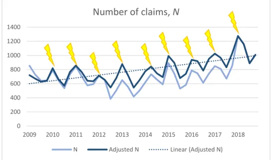
In the end we will have a time series of observations defining the reported claims count at time t representing each time period up to current time T. This time series is illustrated in Figure 5.

Adjustment to current size of the portfolio:

Adjustment factor for observation attached to time 𝑡:

𝑎_𝑡 = 𝑟𝑒𝑙𝑎𝑡𝑖𝑣𝑒 𝑖𝑛𝑐𝑟𝑒𝑎𝑠𝑒 𝑖𝑛 𝑒𝑥𝑝𝑜𝑠𝑢𝑟𝑒 = 𝐸𝑥𝑝𝑜𝑠𝑢𝑟𝑒 𝑎𝑡 𝑐𝑢𝑟𝑟𝑒𝑛𝑡 𝑡𝑖𝑚𝑒 𝐸𝑥𝑝𝑜𝑠𝑢𝑟𝑒 𝑎𝑡 ℎ𝑖𝑠𝑡𝑜𝑟𝑖𝑐𝑎𝑙 𝑡𝑖𝑚𝑒 = 𝐸𝑎𝑟𝑛𝑒𝑑 𝑝𝑟𝑒𝑚𝑖𝑢𝑚𝑇

𝐸𝑎𝑟𝑛𝑒𝑑 𝑝𝑟𝑒𝑚𝑖𝑢𝑚_𝑡 ,

(15)

15

Each historical claim count 𝑛𝑡 is then adjusted to get the claim count given the current portfolio size:

𝑎_𝑡∗ 𝑛_𝑡

This should ideally show a stationary time series, however due to seasonal effects a seasonal time series is expected, with a higher claim count in the winter time. This is

referred to as seasonal effects, or more accurately for this particular case, a winter effect. In Figure 5 the winter effect is highlighted by the yellow lightnings.

Figure 5: Seasonality in the reported claim count

Often in time-series analysis long observation periods are ideal, but in this case the trade-off may be an increase in the bias when the time horizon gets too long. An example of this could be that windscreen technology on cars is changing making windscreens less/more sensitive to breakage.

From the plot above we see a slight increase in the number of claims reported. This linear increase appears to start in 2014. Many factors could potentially cause this. For example, if a company decides to do profitability actions by reducing the profit margin of the risk premium.

E.g. if the price to insure the same risk decreases with time, then given a constant earned premium, more risks will be covered for the same price.

0 200 400 600 800 1000 1200 1400 2009 2010 2011 2012 2013 2014 2015 2016 2017 2018

Number of claims, N

(16)

16

From the Figure 5 we see how this may have been the case from 2014 onwards. However, it is also important to highlight the large diversity among clients and above analysis builds on the assumption that every single client has the same risk ratio and the same profit margin relative to the risk premium.

For industrial clients this is not the case as a large and important client may have a lower profit margin relative to the risk premium compared to the smaller client, as discussed at the end of section 2.3.

The increase may also come from new clients who generate more claims than the others.

2.9 Large claims analysis (> 1 M).

We now leave the low severity-high frequency windscreen claims and proceed to the high severity-low frequency claims, also simply referred to as “large claims”. Large is always a relative term and depends on the overall nature of the portfolio. Some claims may be considered large in a motor portfolio, while in a marine insurance portfolio claims often reach significantly higher severities. This means that the threshold for large claims varies depending on the portfolio.

When pricing an insurance, it is not enough to look at the frequency claims. Often, a large claims loading is added on top of the premium to account for events that have a very large severity, but only occur rarely.

A historical example occurred in Turku, Finland in 2016 when a person set fire to a single bus, parked in a garage among 19 other buses. The 20 buses caught fire causing an estimated

damage of 1 million euros. (YLE 2016)

This loading is based on the large claim analysis. The estimated loss aggregate gives an indication of what the future may bring. But when it comes to pricing individual clients a more profound understanding is needed to be able to assess what risks are reflected in the premium.

It is important to know to what extend the loss aggregate is represented by “high frequency/low severity” claims or “high severity/ low frequency” claims.

(17)

17 high frequency/low severity

An example on this type of claim would be a windscreen damage claim. It is something that occurs to every car owner and is typically independent of the driver’s experience.

high severity/ low frequency

This type of claim happens rarely but when it occurs it is very costly to the insurer. A classic example would be a Bodily injury claim – driver hits another person causing a severe injury.

For the motor portfolio the high frequency claims do not exceed 1 M. It is assumed that this is an appropriate benchmark to separate larger claims from the smaller and more frequent claims.

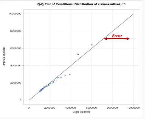
Three motor portfolios have been assessed; Motor portfolio A, B, and C. For Motor portfolio A a truncated lognormal curve was fitted to the loss data above 1 M, right-truncating at 10 M, where no bigger loss has been observed. The accuracy of the fit is shown below in Figure 6.

Figure 6: Q-Q plot of the fitted distribution highlighting the error of the lognormal tail on the claims data from Motor portfolio A.

(18)

18

Figure 6 shows how dominating the tail of lognormal model can be in terms of

overestimating losses. This is seen by the 7 M loss which is estimated to be 10 M. Without the right-truncation point the loss would have been estimated larger.

A reassessment of the inflated loss around 7 M shows that it is an old loss dating back to 2005. In its nature it is a loss belonging to the severity interval [4 M; 6 M]. This could suggest that the loss may be overinflated. Since the majority of the losses in a motor portfolio have a high frequency and low severity the inflation rates will reflect this behaviour, which means that low frequency/high severity losses may suffer from a too high inflation rate.

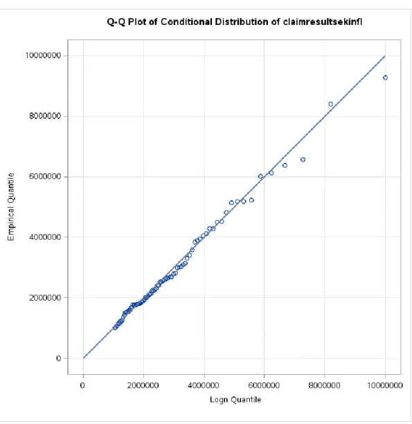
It is stressed that too high inflation rates may not be the answer to this matter, but it is rather a suggestion to further optional research, however beyond the scope of this report. For Motor portfolio B the lognormal model turned out to have the best fit. The final selected model is defined below by its moments and parameters and its quantile to quantile plot is given in Figure 7: Lognormal model: 𝑓_𝑋(𝑥) = 1 𝑥𝜎√2𝜋exp (− (ln|𝑥| − 𝜇)2 2𝜎2 ). 𝜇 = 13.2896 Mean: 2,990,402 𝜎 = 1.80076 Standard deviation: 14,833,023

Proportion of total loss aggregate: 0.066109% (3 large losses per year) (Estimated from observed number of large losses out of total number of losses) Test Statistic:

(19)

19 This gives an annual loading of the motor portfolio of:

𝐸[𝑋𝐿𝑎𝑟𝑔𝑒 𝑙𝑜𝑠𝑠𝑒𝑠] ∗ 𝐸[𝑁𝐿𝑎𝑟𝑔𝑒 𝑙𝑜𝑠𝑠𝑒𝑠] = 2,990,401 ∗ 3

= 8,699,350

Where 𝑋_{𝐿𝑎𝑟𝑔𝑒 𝑙𝑜𝑠𝑠𝑒𝑠} is the severity of the loss and 𝑁_{𝐿𝑎𝑟𝑔𝑒 𝑙𝑜𝑠𝑠𝑒𝑠} is the number of large losses reported.

(20)

20

In Figure 7 above we see that the chosen lognormal distribution fit well on the tail, as the quantiles of the fitted lognormal distribution is close to the quantiles of the empirical distribution.

Fitting a mixed distribution in the tail:

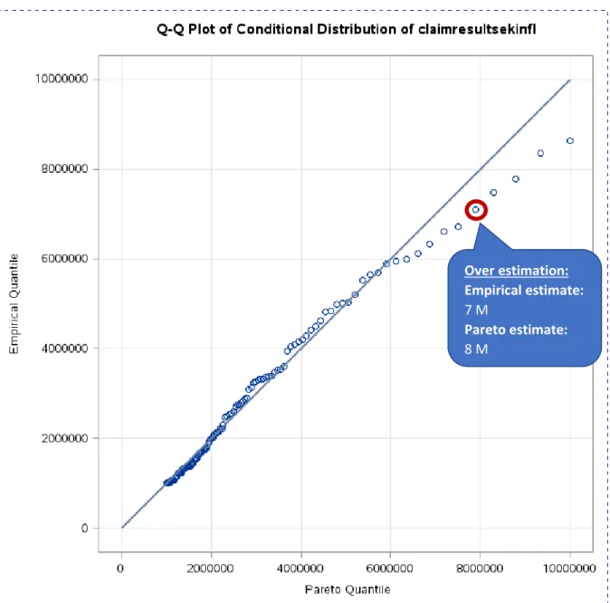
Switching to the analysis of Motor portfolio C, various distributions were fitted in the tail. According to the Kolmogorov-Smirnov and Nelson-Aalen test statistic the Pareto showed the best fit, but from the quantile to quantile plot given in Figure 8 a divergence in the tail can be seen from claims above 6 million. The plot shows how the fitted Pareto distribution is overestimating the large losses just like we saw for Motor portfolio A. For example, a 7 million claim is estimated to be around 8 million by the Pareto model. A remedy to this is to fit another distribution on the claims above 6 million and allow the Pareto model to solely describe the claims belonging to the interval between 1 and 6 million.

(21)

21

Figure 8: Q-Q plot of the distribution fit on another motor claims dataset.

This was concluded from the Quantile to Quantile plot (Figure 8), as the Pareto model had a good fit on the claims below 6 M, however it did not capture the behaviour of the larger claims, and thus the decision of truncating at 6 M and fitting another distribution on the claims above 6 M seemed reasonable.

Refitting various distributions on the losses above 6 M, it was found that the Burr distribution seemed to capture the behaviour of the very large claims.

Hence, the tail of the severity distribution was described by the model defined below: 1 𝑀 < 𝑋_{𝑃𝑎𝑟𝑒𝑡𝑜} < 6 𝑀 Over estimation: Empirical estimate: 7 M Pareto estimate: 8 M

(22)

22

6 𝑀 < 𝑋_{𝐵𝑢𝑟𝑟} < 10 𝑀

Pareto (Type II, Lomax) 𝑓_𝑋(𝑥) = 𝛼𝜃

𝛼 (𝑥 + 𝜃)𝛼+1

Burr (Type XII, Singh-Maddala-type)

𝑓_𝑋(𝑥) = 𝛼𝛾( 𝑥 𝜃)𝛾 𝑥 (1 + (𝑥_𝜃)𝛾) 𝛼+1 𝜃 (𝑠𝑐𝑎𝑙𝑒): 2,960,559 𝛼 (𝑠ℎ𝑎𝑝𝑒): 2.21425 𝜃 (𝑠𝑐𝑎𝑙𝑒): 7,285,579 𝛼 (𝑠ℎ𝑎𝑝𝑒): 1.77679 𝛾 ∶ 7.44365

Each distribution is weighted 103/112 and 9/112 respectively.

This weighting was calculated based on the number of observations which contributed to either the lower or the upper part of the tail.

The overall mean of the tail is obtained using the law of total probability - the weighted average of the conditional means of the two distributions.

𝐸[𝑋_{𝑇𝑎𝑖𝑙}] =103

112∗ 𝐸[𝑋𝑃𝑎𝑟𝑒𝑡𝑜] + 9

112∗ 𝐸[𝑋𝐵𝑢𝑟𝑟] = 2,800,198

It is highlighted that 𝐸[𝑋𝑃𝑎𝑟𝑒𝑡𝑜] and 𝐸[𝑋𝐵𝑢𝑟𝑟] are both conditional expectations, where the conditioning refers to the interval the model was fitted on.

Special property of the Pareto (Type II, Lomax) distribution:

The parameters were initially estimated by maximising the log-likelihood function.

The observations used were given on the interval 1 M to 10 M. However, the losses above 6 M were better represented by the Burr distribution and thus the initial conditional mean should be adjusted such that it only represents the losses below 6 M. The feature illustrated

(23)

23

below shows how this procedure is easily carried out when losses follow a Pareto distribution.

Initial mean: 𝐸[𝑋𝑃𝑎𝑟𝑒𝑡𝑜] = 𝐸[𝑋𝑃𝑎𝑟𝑒𝑡𝑜|𝑢𝑛𝑐𝑜𝑛𝑑𝑖𝑡𝑖𝑜𝑛𝑎𝑙] = 𝜃 𝛼 − 1 = 2,438,179

The new mean is obtained by applying the law of total probability: 𝐴𝑑𝑗𝑢𝑠𝑡𝑒𝑑 𝑚𝑒𝑎𝑛: 𝐸[𝑋_{𝑃𝑎𝑟𝑒𝑡𝑜}|𝑋 < 6 𝑀] = (𝐸[𝑋] − 𝐸[𝑋|𝑋 > 6 𝑀] ∗ Pr(𝑋 > 6 𝑀)) ∗ 1 Pr(𝑋 < 6 𝑀) = ( 𝜃 𝛼 − 1− 𝐸[𝑋|𝑋 > 6 𝑀] ∗ Pr(𝑋 > 6 𝑀)) ∗ 1 Pr(𝑋 < 6 𝑀)

Here the property of a Pareto distributed left-truncated and shifted random variable can be applied, where d = 6 M (Proof given in section 2.10):

𝑒_𝑋(𝑑) = 𝐸[𝑋|𝑋 > 6 𝑀] =∫ 𝑆𝑋(𝑥) 𝑑𝑥 ∞ 𝑑 𝑆𝑋(𝑑) = 𝜃 + 𝑑 𝛼 − 1. (2.5)

By replacing the simplified expression for the mean excess loss (2.5), where 𝑑 = 6 𝑀 into the equation above, we obtain:

𝐸[𝑋_{𝑃𝑎𝑟𝑒𝑡𝑜}|1 𝑀 < 𝑋 < 6 𝑀] = (2,438,179 −𝜃 + 6 𝑀 𝛼 − 1 ∗ 𝑃𝑟(𝑋 > 6 𝑀)) ∗ 1 Pr(𝑋 < 6 𝑀) = (2,438,179 −𝜃 + 6 𝑀 𝛼 − 1 ∗ ( 𝜃𝛼 (6 𝑀 + 𝜃)𝛼)) ∗ 1 1 − (_{(6 𝑀 + 𝜃)}𝜃𝛼 _𝛼) =1,972,616

(24)

24

Note, that the impact is minor since the probability of observing a claim below 6 M is very large, as these very large losses above 6 M rarely occur in a motor portfolio.

2.10 Proof of formula for 𝑒_𝑋(𝑑):

A property of the Pareto distribution is very useful when one needs to assess the impact on the loss distribution upon introduction of deductibles. This property allows us to easily compute the mean excess loss for various deductibles.

It allows us to express the left truncated and shifted variable (also known as the mean excess loss) simply by adding the “shift” to the scale parameter.

This means that to get the distribution obtained above (Pareto distribution fitted on the interval 1 M to infinity, we left truncate at 1 M, which can be imagined as a deductible d i.e. we do not consider payments below d = 1 M.

The mean excess loss 𝑒𝑋(𝑑) of the random variable X~Pareto(𝛼; 𝜃), given deductible d is defined below according to Klugman, Panjer and Willmot (2012) and the proof was outlined by the course notes obtained from the Master of Actuarial Science programme from University of Manitoba: 𝑒_𝑋(𝑑) = ∫ 𝑆𝑋(𝑥) 𝑑𝑥 ∞ 𝑑 𝑆_𝑋(𝑑) = ∫ 𝜃 𝛼 (𝑥 + 𝜃)𝛼 𝑑𝑥 ∞ 𝑑 𝜃𝛼 (𝑑 + 𝜃)𝛼 = 𝜃𝛼_∫ 1 (𝑥 + 𝜃)𝛼 𝑑𝑥 ∞ 𝑑 𝜃𝛼 (𝑑 + 𝜃)𝛼

Assuming the shape parameter 𝛼 > 1, the integral of the survival function, i.e. the expected value considering the domain above the deductible d, is given by a closed form:

∫ 𝑆_𝑋(𝑥) 𝑑𝑥 ∞ 𝑑 = 𝜃𝛼_∫ 1 (𝑥 + 𝜃)𝛼 𝑑𝑥 ∞ 𝑑 = ( 𝜃 𝛼 𝛼 − 1) ∗ ( 1 (𝑑 + 𝜃)𝛼−1)

(25)

25

When solving the integral of the survival function given in the numerator the expression simplifies which yields the mean excess loss given a deductible d:

= ( 𝜃 𝛼 𝛼 − 1) ∗ (_{(𝑑 + 𝜃)}1 _𝛼−1) 𝜃𝛼 (𝑑 + 𝜃)𝛼 =𝜃 + 𝑑 𝛼 − 1 ∎ 2.11 Result.

We leave the theory and proceed with the analysis of the large losses.

We see from the large claim loading that losses above 1 M make up a very small proportion of the total portfolio. However, they do occur more often than once a year.

But in comparison to the aggregate severity of the overall portfolio it can be concluded that the loss aggregate is primarily driven by high-frequency/low severity claims rather than the infrequent, large losses.

Below is a breakdown of how much of the Risk Ratio that is driven by large claims (claims > 1 M). 𝑅𝑖𝑠𝑘 𝑅𝑎𝑡𝑖𝑜 (𝑅𝑅) = 𝐿𝑜𝑠𝑠 𝐴𝑔𝑔𝑟𝑒𝑔𝑎𝑡𝑒 𝐸𝑎𝑟𝑛𝑒𝑑 𝑃𝑟𝑒𝑚𝑖𝑢𝑚 𝑅𝑅_{𝑆𝑤𝑒𝑑𝑒𝑛} =𝐸𝑥𝑝𝑒𝑐𝑡𝑒𝑑 𝑡𝑎𝑖𝑙 𝑠𝑒𝑣𝑒𝑟𝑖𝑡𝑦 ∗ 𝐸𝑥𝑝𝑒𝑐𝑡𝑒𝑑 𝑛𝑢𝑚𝑏𝑒𝑟 𝑜𝑓 𝑙𝑎𝑟𝑔𝑒 𝑙𝑜𝑠𝑠𝑒𝑠 𝐸𝑎𝑟𝑛𝑒𝑑 𝑝𝑟𝑒𝑚𝑖𝑢𝑚 = 10 % 𝑅𝑅𝐹𝑖𝑛𝑙𝑎𝑛𝑑 = 12 % 𝑅𝑅_{𝑁𝑜𝑟𝑤𝑎𝑦} = 15 % 𝑅𝑅_{𝐷𝑒𝑛𝑚𝑎𝑟𝑘} = 13 %

(26)

26 2.12 Estimating future losses.

When a policy is written the insurer holds the obligation to cover the losses, defined in the insurance policy, given they occur within the policy period. This obligation holds regardless of the date that the policyholder notifies the insurance company about the loss.

The period between the loss occurrence date and the reporting date is referred to as

reporting delay. This delay is usually short in a motor portfolio, but there may be reasons for the policyholder not to report the claim immediately.

As a consequence, a group of claims can be referred to as IBNR – claims Incurred But Not Reported. When a claim has incurred the event giving rise to the claim has occurred but when the claim has not reported it means that the claim has not been notified to the insurer. This means that the insurer has a future obligation to pay for a claim which the insurer is unaware of. In this section it is shown that this amount is not of a negligible amount. In fact, it may be rather significant. Hence, it is crucial for the insurer to build sufficient reserves that account for these obligations.

A set of assumptions must be set, and a common standard is to assume, that the claims follow the stochastic discreet time Poisson process, described by Taylor & Karlin (1998). The Poisson process describes the pattern in which the claim’s arrival follows. When a claim arrives, it means that the claim has been reported. In addition, we can observe, once a claim has been reported, how long it takes to settle the claim. A claim is settled, once no more payments will follow. Often claim payments are done all at once, but there are cases where the claim payments are broken down into several payments. An example for this is in the case of injury, where the injured has right to annuity payments, to compensate for loss of income when the injury is so severe that the injured is unable to work. In these cases, it will take a longer time to settle a claim.

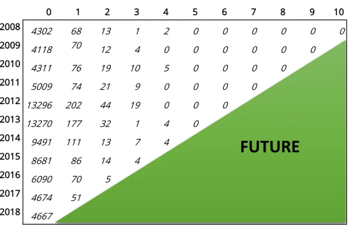
Given the assumptions of the Poisson process we can group all our settled claims by the time they were reported and by the time it took to settle them. A visualisation of this

grouping is illustrated in the development triangle (see Figure 9) which contains the number of reported claims.

(27)

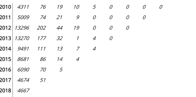
27 0 1 2 3 4 5 6 7 8 9 10 2008 4302 68 13 1 2 0 0 0 0 0 0 2009 4118 70 ₁₂ ₄ ₀ ₀ ₀ ₀ ₀ ₀ 2010 4311 76 19 10 5 0 0 0 0 2011 5009 74 21 9 0 0 0 0 2012 13296 202 44 19 0 0 0 2013 13270 177 32 1 4 0 2014 9491 111 13 7 4 2015 8681 86 14 4 2016 6090 70 5 2017 4674 51 2018 4667

Figure 9: Incremental development triangle containing claim count data. A lot of different mathematical and statistical methods makes it is possible to project the experienced claims and obtain an expectation on the final payments in the future – the so-called ultimate. The experience is tracked by the claim’s settlement-delay (Settlement date – Reporting date), which in the development triangle in Figure 9 is given by each column. A Chain-ladder model uses the claim count to compute the expected number of claims IBNR (incurred but not reported). The definitions and the Chain-ladder model procedure is in line with Neuhaus (2014), although notation has been altered. The claims are grouped according to their delay and we assume independence between the delay-intervals. It then estimates an average growth rate for each delay and applies it to the aggregated claim count to obtain the result – the claim ultimate.

Figure 9 illustrates how the claims are grouped. Each column represents the delay of the observed claim while the row assigns the reporting year. This gives the data its characteristic triangular shape, representing the past (upper triangle) and the future (lower triangle.

By iteratively aggregating each horizontal entry in the incremental development triangle in Figure 10 we obtain the cumulative development triangle (Figure 11).

(28)

28

From the cumulative development triangle each proceeding column no longer shows the increase but instead the aggregate.

0 1 2 3 4 5 6 7 8 9 10

2008 4302 68 13 1 2 0 0 0 0 0 0

(29)

29 2010 4311 76 19 10 5 0 0 0 0 2011 5009 74 21 9 0 0 0 0 2012 13296 202 44 19 0 0 0 2013 13270 177 32 1 4 0 2014 9491 111 13 7 4 2015 8681 86 14 4 2016 6090 70 5 2017 4674 51 2018 4667

Figure 10: Incremental development triangle containing the claim count data. Adjustment of each entry for portfolio size (Exposure).

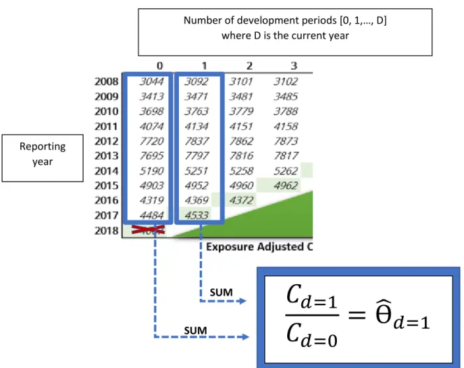
0 1 2 3 4 5 6 7 8 9 10 2008 3044 3092 3101 3102 3103 3103 3103 3103 3103 3103 3103 2009 3413 3471 3481 3485 3485 3485 3485 3485 3485 3485 2010 3698 3763 3779 3788 3792 3792 3792 3792 3792 2011 4074 4134 4151 4158 4158 4158 4158 4158 2012 7720 7837 7862 7873 7873 7873 7873 2013 7695 7797 7816 7817 7819 7819 2014 5190 5251 5258 5262 5264 2015 4903 4952 4960 4962 2016 4319 4369 4372 2017 4484 4533 2018 4667

Figure 11: Exposure adjusted cumulative development triangle.

In the highlighted (light green) diagonal the entries represent the total claim count at

current point in time. It is this aggregate which we wish to project into the future, so we can obtain the final claim count ultimate.

(30)

30

To highlight how intuitive the Chain-ladder is Figure 12 illustrates the procedure of estimating the development factors. This also avoids the complicated notation which follows from an otherwise rather simple and intuitive model.

Figure 12: Illustration of the Chain-ladder estimation procedure of the claim’s development factor.

In Figure 12 the development factors, Ө̂𝑑, 𝑑 = 1, 2, … , 𝐷 are estimated. Given the assumption of independence between claims which have different delay the relative growth Ө̂𝑑 given development d is estimated by the ratio of the total number of claims 𝐶𝑑, observed within each delay-group d.

SUM SUM

𝐶

_𝑑=1

𝐶

_𝑑=0

= Ө

̂

𝑑=1

Number of development periods [0, 1,…, D] where D is the current year

Reporting year

(31)

31

Figure 13: Claims development factor Ө̂𝑑. As the development factor approaches 1 the ultimate is reached, and no more claims are expected to be reported.

From the plot above, the typical pattern for the development factor is shown. Here it can be seen that the portfolio is quite short tailed as nearly all claims are reported within the first two development periods. Since the Chain-ladder model measures the increase between two intervals of delay it is very sensitive. This means that for portfolios with a longer tail where claims develop for a much longer period a Chain ladder procedure may result in a “wagging” tail since minor changes in the early development years will impact all the way out in the later development years.

Since we have already established from Figure 13 that our portfolio is short-tailed the final step of the Chain-ladder is carried out – projecting the diagonal in the development triangle using the estimated development factors. This yields the lower triangle entries shown in Figure 14, where the ultimate is given in the right-most column.

1 1,002 1,004 1,006 1,008 1,01 1,012 1,014 1 2 3 4 5 6 7 8 9 10 Development periods

Development factor

(32)

32

Figure 14: Completed cumulative development triangle containing the estimated ultimate number of claims in the highlighted column furthest to the right. The diagonal is highlighted

in green, which separates the observations from the estimates.

This ultimate highlighted with a blue frame represents the total number of claims which we can expect to be liable for.

Reassessing the completed cumulative claims development triangle, the ultimate number of claims is given in the right-most column. The difference between the currently observed number of claims (green diagonal) and the ultimate yields the number of claims we expect to be reported in the future.

0 1 2 3 4 5 6 7 8 9 10 2008 3044 3092 3101 3102 3103 3103 3103 3103 3103 3103 3103 2009 3413 3471 3481 3485 3485 3485 3485 3485 3485 3485 3485 2010 3698 3763 3779 3788 3792 3792 3792 3792 3792 3792 3792 2011 4074 4134 4151 4158 4158 4158 4158 4158 4158 4158 4158 2012 7720 7837 7862 7873 7873 7873 7873 7873 7873 7873 7873 2013 7695 7797 7816 7817 7819 7819 7819 7819 7819 7819 7819 2014 5190 5251 5258 5262 5264 5264 5264 5264 5264 5264 5264 2015 4903 4952 4960 4962 4964 4964 4964 4964 4964 4964 4964 2016 4319 4369 4372 4376 4378 4378 4378 4378 4378 4378 4378 2017 4484 4533 4545 4549 4550 4550 4550 4550 4550 4550 4550 2018 4667 4730 4743 4747 4748 4748 4748 4748 4748 4748 4748

Ultimate

(33)

33

Figure 15: Summary of the results from the Chain-ladder model From the table we see that we can expect 105 claims to be reported in the future:

Total expected number of claims IBNS = 1 + 5 + 17 + 81 = 104

We see that this quick settlement in motor results in a very short-tailed business and thus the expected IBNR is quite low.

For the Normal Year 2020 loss estimate we need to add some of this expected IBNR on top of our estimated loss, since we expect to pay for some of these IBNR claims in 2020. This amount is simply calculated by the product of the expected IBNR and the expected average loss. Same reserving procedure (Chain-ladder) may also be applied to a development triangle containing the historical payments. This will also yield an expectation of the payments IBNR. Diagonal (Most recent observation) Ultimate Triangle diagonal 2008 3103 3103 0 2009 3485 3485 0 2010 3792 3792 0 2011 4158 4158 0 2012 7873 7873 0 2013 7819 7819 0 2014 5264 5264 0 2015 4962 4964 1 2016 4372 4378 5 2017 4533 4550 17 2018 4667 4748 81

(34)

34

3. Claim adjustment reserve analysis

In addition to the claim payments, the insurance company carries costs for assessing the severity of the claims. This is called the claims handling process and this process can for some claims be long and costly to the insurer. Not only does the normal administrative part of the claim reporting take time, but some more complicated claims require significant expert assessment.

An example in Marine insurance, may be to have a marine biologist to investigate the damages caused by oil spill from a damaged hull as well as an engineer to assess the

damaged/undamaged cargo as some undamaged cargo is potential for reselling. What follows from this process is known as claims handling cost.

These claim’s handling costs are known for settled claims but for outstanding claims (incurred but non-reported claims as well as open claims) one must set reserves for the expected future claim’s handling costs. This reserve is commonly known as claim adjustment reserve (CAR).

Each line of business (Motor, Marine, Property, Liability etc.) has a very different nature and some require a lot higher CAR compared to others.

A model was built for further assessment of the historical claim adjustment reserves. This model matches the CAR with the current proportion of paid claims handling cost.

The following section will dig further into the performance of this model and how it impacts the currently booked CAR.

(35)

35 3.1 Establishing terminology

Claim adjustment reserve (CAR) is assumed a fixed percentage of the IBNS (incurred but not settled) 𝐼𝐵𝑁𝑆 = { 𝐼𝐵𝑁𝑅 + 𝐶𝑎𝑠𝑒 𝑟𝑒𝑠𝑒𝑟𝑣𝑒 = { 𝑝𝑢𝑟𝑒 𝐼𝐵𝑁𝑅 (𝐼𝑛𝑐𝑢𝑟𝑟𝑒𝑑 𝑏𝑢𝑡 𝑛𝑜𝑡 𝑟𝑒𝑝𝑜𝑟𝑡𝑒𝑑) + 𝐼𝐵𝑁𝐸𝑅 (𝐼𝑛𝑐𝑢𝑟𝑟𝑒𝑑 𝑏𝑢𝑡 𝑛𝑜𝑡 𝑒𝑛𝑜𝑢𝑔ℎ 𝑟𝑒𝑝𝑜𝑟𝑡𝑒𝑑) + 𝐶𝑎𝑠𝑒 𝑟𝑒𝑠𝑒𝑟𝑣𝑒 . (3.1)

The understanding of the used acronyms IBNER and IBNS is in line with the definitions given in Neuhaus (2014), while IBNR describes the estimated outstanding claims excluding the case reserves (IBNR = IBNS – case reserve = pure IBNR + IBNER).

Pure IBNR: “Incurred But Not Reported” in the strict sense defines claims where the event that will give rise to a claim (fire, theft, vehicle damage, etc.) has occurred, but where the claim has not been notified to the insurer. In some literature this is referred to as IBNyR (incurred but not yet reported).

In insurance accounting it is common to use the term IBNR for the expected increase (in some cases, decrease) in booked cost, over and above payments already made and case reserves, that will have occurred by the time all claims of a cohort are settled. In other words, accountants use the term IBNR to describe that part of the outstanding claim cost, that has not been recognised as case estimates. This means that IBNR = Predicted ultimate claim cost – Case reserves – claim payments = IBNS – Case reserves.

Case reserve: describes the assumed reserve attached to all open claims.

IBNER + Case reserves:includes all open claims together with reopened claims. For the CAR-model this is the booked Case reserves attached to all open claims.

IBNER describes the future development of reported claims. That is, once a claim has been reported (but not settled) and case reserves have been built based on the information we know about the claim, there is a remaining part of the total claim payment which is not reflected by the case reserve. This remaining part could arise if the damage from which the

(36)

36

claim arises turns out to be more severe than previously believed.

Example: How IBNER incurs to the insurer.

Upon bodily injury following from a car accident, the doctors may discover that the injuries were more severe than previously believed. This would make the claim payment increase by some amount such that the new claim payment reflects the severity of the hazard. This increase in the claim payment is the IBNER part of the open claim.

3.2 Assumptions.

Upon assessment of CAR-model the following assumptions are made:

3.2.1 Open claims.

Open claims are the claims notified to the insurer and which are still under current processing. This processing may be an expert assessment of the severity of the damage caused by the claim cause (e.g. Third-party liability - Bodily injury claims: Percentage of invalidity, Cargo claims: proportion of goods damaged and whether undamaged/saved goods are eligible for reselling).

This means that reopened claims are treated as new claims.

3.2.2 Capping.

Although the claims handling cost is often given as a fixed percentage of the claim severity, a large claim may not cost more to settle than another large claim, even if the two claims may differ by a 100K Euros in severity.

E.g. a 100 MEUR claim does not cost 100 times more to settle compared to a 1 MEUR claim. To account for this, large claims have been truncated (capped). This means effectively that the reserves set for handling very large claims (the ones above the threshold) are the same irrespective of the claim severity. Another assumption is that any single claim should not

(37)

37

require a claim handling cost larger than approximately the cost (salary) of a senior claims-handler for an entire year (including overheads).

Below is the simplified CAR model illustrated. It can be seen how the IBNS and the claim handling cost ratio make up the assumed proportion of CAR.

𝐶𝐴𝑅 =𝑝𝑎𝑖𝑑 𝑐𝑙𝑎𝑖𝑚 ℎ𝑎𝑛𝑑𝑙𝑖𝑛𝑔 𝑐𝑜𝑠𝑡

𝑐𝑎𝑝𝑝𝑒𝑑 𝑝𝑎𝑦𝑚𝑒𝑛𝑡𝑠 ∗ 𝐶𝑎𝑝𝑝𝑒𝑑 𝐼𝐵𝑁𝑆

(3.2)

= 𝑝𝑎𝑖𝑑 𝑐𝑙𝑎𝑖𝑚 ℎ𝑎𝑛𝑑𝑙𝑖𝑛𝑔 𝑐𝑜𝑠𝑡

𝑐𝑎𝑝𝑝𝑒𝑑 𝑝𝑎𝑦𝑚𝑒𝑛𝑡𝑠 ∗ [𝑝𝑢𝑟𝑒 𝐼𝐵𝑁𝑅 + 𝐼𝐵𝑁𝐸𝑅 + 𝐶𝑎𝑝𝑝𝑒𝑑 𝐶𝑎𝑠𝑒 𝑟𝑒𝑠𝑒𝑟𝑣𝑒].

According to assumption defined in 3.2.2 the Case reserve includes case reserves higher than the limit (cap) we’ve set. These cases which are in excess of the cap must be deducted from the Case reserve resulting in Capped Case reserve.

We do not consider that settled claims can be reopened. Upon reopening of a claim, the claim will be considered a new claim. It is highlighted that this is a strong assumption as it assumes that no claim handling cost has been paid for this new claim, when in fact some claim’s handling costs has already been covered during the previous claim’s handling process.

(38)

38 3.2.2.1 Capping Example.

Figure 16: The capping procedure of the CAR-model.

For one of the portfolios analysed, two capping limits are given. These capping limits represent approximately the annual salary of a senior claim’s handler.

Figure 16 is a visualisation of the loss capping procedure. It highlights that the capped amount is conditional on the assumed CAR%, which is the CAR expressed as a percentage rather than a nominal value. This procedure is performed by a Macro in SAS and the result is extracted in the form of the amount in excess of the capping limit.

As the previously booked CAR% was given by 3% one can calculate the total amount the in excess of the capping point the following way:

Total claim payments = 100

CAR% = 3%

Capping limit = 1

𝐶𝐴𝑅 = 3% ∗ 100 = 3 Amount capped = 3 − 1 = 2

Total amount in excess of the capping limit = 2 / 3% = 66.667

What is important to note here is that we are assuming that no claim takes more than an entire year’s work to settle.

Capped claim

payments

66.67

(amount in excess of capping limit)

Capped claim

payments

Total claim

payments

100

3 % Capping limit

(39)

39 3.3 The CAR model.

Processing above assumptions we proceed with the actual model.

The CAR model builds on the “New York-method”. The model assumes that CAR is proportional to the claim payments.

Hence, by assuming that CAR% is equal to the claim’s handling cost ratio (Cost/Paid ratio) we can obtain the nominal amount required to reserve for Claim’s adjustment.

𝐶𝐴𝑅% = 𝑃𝑎𝑖𝑑 𝑐𝑙𝑎𝑖𝑚 ℎ𝑎𝑛𝑑𝑙𝑖𝑛𝑔 𝑐𝑜𝑠𝑡𝑠 𝐶𝑎𝑝𝑝𝑒𝑑 𝑃𝑎𝑦𝑚𝑒𝑛𝑡𝑠 → 𝐶𝐴𝑅 = 𝐶𝐴𝑅% ∗ 𝑂𝑢𝑡𝑠𝑡𝑎𝑛𝑑𝑖𝑛𝑔 𝑝𝑎𝑦𝑚𝑒𝑛𝑡𝑠 = 𝐶𝐴𝑅% ∗ ((1 − 𝑦) ⋅ 𝐼𝐵𝑁𝑅_{𝑏𝑜𝑜𝑘𝑒𝑑}+ 𝑥 ∗ (𝑦 ∗ 𝐼𝐵𝑁𝑅_{𝑏𝑜𝑜𝑘𝑒𝑑}+ 𝐶𝑎𝑝𝑝𝑒𝑑 𝐶𝑎𝑠𝑒 𝑟𝑒𝑠𝑒𝑟𝑣𝑒)) = 𝐶𝐴𝑅% ∗ (𝑝𝑢𝑟𝑒 𝐼𝐵𝑁𝑅 + 𝑥 ∗ (𝐼𝐵𝑁𝐸𝑅 + 𝐶𝑎𝑝𝑝𝑒𝑑 𝐶𝑎𝑠𝑒 𝑟𝑒𝑠𝑒𝑟𝑣𝑒)) ⋅

𝐶𝑎𝑝𝑝𝑒𝑑 𝐶𝑎𝑠𝑒 𝑟𝑒𝑠𝑒𝑟𝑣𝑒 is the part of the case reserve remaining after capping according to the capping rule defined above in section 3.2.2.1.

Capped payments describe the part of the payment remaining after capping according to the capping rule defined above in section 3.2.2.1.

Parameter y: is the parameter defining the proportion of booked IBNR which is IBNER according to the split defined in (3.1).

Parameter x: denotes the outstanding proportion of the costs for handling reported claims i.e. 𝑥 ∗ (𝐼𝐵𝑁𝐸𝑅 + 𝐶𝑎𝑝𝑝𝑒𝑑 𝑐𝑎𝑠𝑒) is the amount yet to be paid. It may be reasonable to assume that half of the ultimate has been paid. That is, a linear development of the claim cost process. This is merely simplicity rather than reality. To explain in other words, this means that the CAR% (ratio of future claim handling cost to future claim payments) is only half as large for claims that have already been reported, as for claims that will be reported in the future.

The initial parameter assumptions are in line with Buchwalder et al. (2006) describing the New York-method.

(40)

40

From the basis of this model explained above the following analysis will assess the sensitivity of the Claim Adjustment Reserves of the Swedish Industrial Liability insurance portfolio.

3.4 Adjusting the initial CAR estimate.

The new CAR% estimate is obtained by setting the initial CAR% equal to the Cost/Paid ratio (the ratio between the actual paid claim-handling costs and the capped claim payments). To reiterate, CAR is the claim-handling cost attached to the booked reserve IBNS.

In defence of the model, one could argue that the same claim, which already occurred, would intuitively cost the same if it were to be reported in the future.

Hence, it is assumed that the proportion of claim-handling costs paid would be the same for the claims which are yet to be reported.

Initial parameter assumptions:

• y: Initially, we assume that 50 % of the booked IBNR is IBNER, which implies y = 50 %. Hence, IBNR is made up by equal parts of pure IBNR and IBNER.

• x: Initially, we assume that 50 % of the costs for handling the settlement of claims IBNER and Capped case has already been paid, which implies x = 50 %.

For each portfolio analysed initial estimates were computed. The initial results are left out of this section as the impact of the x- and y-parameters are studied in section 3.9.

3.5 Assessment of two portfolios for CAR.

Two diverse portfolios were assessed to measure the impact of changing the CAR-model - the Liability portfolio and the Property damage portfolio. Both portfolios are diverse in the sense that their nature causes their reserves to differ. The Liability portfolio has much larger reserves compared to the Property portfolio. Since the reserves are used to compute the CAR, the two diverse portfolios would capture the impacts of introducing the new

(41)

CAR-Master’s Final Work Master of Actuarial Science Casper Jacob Moerup

41 model under different reserve conditions.

3.6 Parameter sensitivity

The CAR-model consists of two main parameters, x and y (see definition above in section 3.4). Below is an example illustrating how impactful the x-parameter is and how the y-parameter in some cases become superfluous.

We see below that any reduction in the expected IBNER amount will reduce the CAR%, which is the estimated CAR given as a percentage.

𝐶𝐴𝑅% = 𝐶𝑜𝑠𝑡 𝑃𝑎𝑖𝑑∗ (𝑥 ∗ (𝐼𝐵𝑁𝐸𝑅 + 𝐶𝑎𝑝𝑝𝑒𝑑 𝑐𝑎𝑠𝑒) + 𝑝𝑢𝑟𝑒 𝐼𝐵𝑁𝑅) 𝐶𝑎𝑝𝑝𝑒𝑑 𝐼𝐵𝑁𝑆 = 𝐶𝑜𝑠𝑡 𝑃𝑎𝑖𝑑∗ 𝑎𝑑𝑗𝑢𝑠𝑡𝑚𝑒𝑛𝑡 𝑓𝑎𝑐𝑡𝑜𝑟 𝑎𝑐𝑐𝑜𝑢𝑛𝑡𝑖𝑛𝑔 𝑓𝑜𝑟 𝑑𝑒𝑣𝑒𝑙𝑜𝑝𝑚𝑒𝑛𝑡 𝑎𝑛𝑑 𝑐𝑎𝑝𝑝𝑖𝑛𝑔. Where, 𝐼𝐵𝑁𝑆 = 𝐶𝑎𝑠𝑒 𝑟𝑒𝑠𝑒𝑟𝑣𝑒 + 𝐼𝐵𝑁𝐸𝑅 + 𝑝𝑢𝑟𝑒 𝐼𝐵𝑁𝑅. 𝐼𝐵𝑁𝐸𝑅 = 𝑦 ∗ 𝐼𝐵𝑁𝑅. 𝑝𝑢𝑟𝑒 𝐼𝐵𝑁𝑅 = (1 − 𝑦) ∗ 𝐼𝐵𝑁𝑅.

Below, are the outputs from the CAR-model when adjusting the parameters x, and y. The impact is measured by assessing four extreme events:

➢ x = y = 0 % : Open claims are fully handled and no open claims. ➢ x = y = 100 % : Open claims have not been handled and all

outstanding claims are open claims (no IBNR). ➢ x = 0 % and y = 100 % : Open claims are fully handled and all outstanding

claims are open claims (no IBNR).

➢ x = 100 % and y = 0 % : Open claims are fully handled and no open claims. Clearly the open claims are neither 100 % handled nor unhandled. Neither can we expect no IBNR nor no open claims. Hence, it would be illuminating to assume something in the

(42)

42

Two portfolios with differing IBNS are assessed, to highlight the impact of IBNS on the parameters. It can also be seen how the high IBNS strengthens the impact from the y-parameter.

Liability: High IBNR

If all open claims are fully handled; 𝑥 = 0 %:

𝑦 = 0 % -> CAR% = 3.6 %

𝑦 = 100 % -> CAR% = 3.6 %

We see that when all open claims are fully handled the y-parameter has no purpose. This is because regardless of the amount of IBNER we have, all claims are fully handled and thus require no reserve.

If all claims IBNER are unhandled; 𝑥 = 100 %:

𝑦 = 0 % -> CAR% = 2.7 %

𝑦 = 100 % -> CAR% = 0.0 %

Property: LOW IBNR

If all open claims are fully handled; 𝑥 = 0 %:

𝑦 = 0 % -> CAR% = 2.2 %

𝑦 = 100 % -> CAR% = 2.2 %

If all claims IBNER are partly unhandled; 𝑥 = 100 %:

𝑦 = 0 % -> CAR% = -0.1 %

𝑦 = 100 % -> CAR% = 0.0 %

From the two outputs from the Property portfolio above we see that the y-parameter has minimal impact when IBNR is low.

(43)

43

The CAR-formula imposes that the impact of the y-parameter increases as parameter 𝑥 → 1, which can also be deduced from the example above.

The model calculates CAR based on two main components: IBNR and RBNS, which can be retrieved through the use of a 3-dimensional reserving model rather than a traditional 2-dimensional model such as the Chain-ladder model (section 2.12).

The y-parameter defines the proportion of IBNR that is IBNER which then is adjusted by the x-parameter.

When IBNR is small so will be the contribution to IBNER from the y-parameter and thus the impact from the x-parameter will also be small.

Figure 18 below highlights how the CAR will be highly unaffected by the y-parameter when the IBNR is small as there simply will not be much IBNER to adjust.

In conclusion, a split between pure IBNR and IBNER is unnecessary when the IBNR is small.

Figure 18: Illustration of the impact of the y-parameter (transferring claims IBNER from IBNR). The result is a split of IBNR into IBNER and pure IBNR.

But when it comes to reserving it is hard to know whether IBNR will be high or low before picking reserving model. Usually, the actuary will have an intuition from the past experience of the portfolio.

3.7 Impact of changing CAR

The following initial results from the model are obtained through fixing the assumptions: Date: 2019-03

Parameters: x = y = 50 %

y

(44)

44 The model suggests the following:

CAR% Claim’s handling cost ratio

Liability SE 2.9% (Previously: 3.0%) 4.5%

Property SE 1.2% (Previously: 4.4%) 2.9%

Figure 19: Results from the CAR-model.

From the table of results given above it is clear from the CAR% column that the impact of adjusting the CAR and assuming it proportional to the cost/paid ratio reduces the CAR.

3.8 Assessing the assumption: CAR is proportional to Cost/Paid ratio

The purpose of “Adj. CAR%” (red graph in Figure 20 and 21) is to get a CAR% that is comparable to the Cost/Paid ratio (blue graph in Figure 20 and 21).

We can then from Figure 20 and 21 assess our assumption on how the CAR% follows the Cost/Paid ratio. A more volatile Cost/Paid ratio would imply a need for frequent update of the CAR. This is because we wish to use the most recent trend of the Cost/Paid ratio, to assure that our CAR is up-to-date.

Hence, for the purpose of this model we do not really need to worry much about the historical volatility of the Cost/Paid ratio. If a sudden jump is experienced, we may not necessarily adjust our Adj. CAR% to experience the same jump (unless we wish to update our CAR continuously).

For the Liability portfolio this assumption appears to hold and thus the CAR% should be equal to the Cost/Paid ratio.

(45)

45

Figure 20: Comparison of the CAR% with the Cost/Paid ratio for the Liability portfolio.

Figure 21: Comparison of the CAR% with the Cost/Paid ratio for the Property portfolio. This is, however, not the case for the Property portfolio. We see that the adjusted CAR% lies way above the Cost/Paid ratio, partially due to the negative IBNR as well as the low case reserves and large caps.

𝐴𝑐𝑡𝑢𝑎𝑙 𝐶𝐴𝑅% = 𝑃𝑎𝑖𝑑 𝐶𝐴𝑅 𝐼𝐵𝑁𝑆 = 𝑃𝑎𝑖𝑑 𝐶𝐴𝑅 𝐼𝐵𝑁𝑅 + 𝐶𝑎𝑝𝑝𝑒𝑑 𝐶𝑎𝑠𝑒 𝑟𝑒𝑠𝑒𝑟𝑣𝑒 0,0% 2,0% 4,0% 6,0% 8,0% 10,0% 12,0% 2019-12 2019-10 2019-08 2019-06 2019-04 2019-02 2018-12 2018-10 20 18 -08 20 18 -06 2018-04 2018-02 2017-12 2017-10 2017-08 2017-06 2017-04 2017-02 2016-12 2016-10 2016-08 2016-06 2016-04 2016-02 2015-12 2015-10 2015-08 2015-06 2015-04 2015-02

Liability: Adj. CAR%

Costs/Paid Adj. CAR% New Adj. CAR%

-10,0% -5,0% 0,0% 5,0% 10,0% 15,0% 2019-12 2019-10 2019-08 2019-06 2019-04 2019-02 2018-12 2018-10 2018-08 2018-06 2018-04 2018-02 2017-12 2017-10 2017-08 2017-06 2017-04 2017-02 2016-12 2016-10 2016-08 2016-06 2016-04 2016-02 2015-12 2015-10 2015-08 2015-06 20 15 -04 2015-02

Property: Adj. CAR%

Costs/Paid Adj. CAR% New Adj. CAR%

We align our CAR according to the most recent Cost/Paid ratio trend.

Prediction of claim cost in general insurance

M

ASTER

MASTER

OF

ACTUARIAL

SCIENCE

M

ASTER

´

S

F

INAL

W

ORK

INTERNSHIP

REPORT

PREDICTION

OF

CLAIM

COST

IN

GENERAL

INSURANCE

CASPER

JACOB

MOERUP

S

:

W

N

(ISEG)

A

T

(I

P&C

I

)

Table of contents

1. Introduction

2. Normal Year 2020 analysis

Premium/Risk

exchange

Insurer

Policy holders

RR

Portfolio

RR

Portfolio

Number of claims, N

𝐶

𝑑=1

𝐶

𝑑=0

= Ө

̂

𝑑=1

Development factor

Ultimate

3. Claim adjustment reserve analysis

Capped claim

payments

66.67

Capped claim

payments

Total claim

payments

100

y

Liability: Adj. CAR%

Property: Adj. CAR%

_𝑑=1

_𝑑=0