SNP detection in F3H gene of Vitis vinifera L. for varietal identification using HRM and biosensors

Universidade de Trás-os-Montes e Alto Douro

SNP detection in F3H gene of Vitis vinifera L. for varietal

identification using HRM and biosensors

Dissertação de Mestrado em Genética Molecular Comparativa e Tecnológica

Cláudia Manuela Oliveira Castro

Orientadora: Professora Doutora Paula Filomena Martins Lopes

Co-orientadora: Doutora Sónia Maria Alves Gomes

ii

Universidade de Trás-os-Montes e Alto Douro

SNP detection in F3H gene of Vitis vinifera L. for varietal

identification using HRM and biosensors

Dissertação de Mestrado em Genética Molecular Comparativa e Tecnológica

Cláudia Manuela Oliveira Castro

Orientadora: Professora Doutora Paula Filomena Martins Lopes

Co-orientadora: Doutora Sónia Maria Alves Gomes

Composição do Júri:

________________________________________

________________________________________

________________________________________

________________________________________

________________________________________

Vila Real, 2015

iii

Acknowledgments

This work would have not be possible without the help and support of several people and institutions, which I want to sincerely thank:

To the Dean of University of Trás-os-Montes and Alto Douro (UTAD), Professor António Fontainhas Fernandes, Ph.D., for the opportunity to conduct the research in this institution;

To the Department of Genetics and Biotechnology and the Department of Physics of UTAD, for allowing the use of its facilities and materials;

To the BioISI Center, where I have developed my research.

To the FCT (Fundação para a Ciência e Tecnologia) through the funding of the project “Biosensor Development for Wine Traceability in the Douro Region (WineBioCode)”

(PTDC/AGR-ALI/117341/2010- -FCOMP-01-0124-FEDER-019439).

To Professor Paula Filomena Martins Lopes, Ph.D., my supervisor, for the unceasing support, counselling, help and motivation;

To Sónia Maria Alves Gomes, Ph.D., my co-supervisor, for stepping in and always helping me in as much as I needed;

To Professor José Ramiro Fernandes, Ph.D., for helping me with all the work involving the biosensor;

To Leonor Pereira, MSc., and Helena Rodrigues, Ph.D., for always finding time in their busy schedule to clarify doubts;

To my mother, Conceição Oliveira, for supporting my education all these years and loving me unconditionally;

To my family, especially my Aunt Manuela Vila-Pouca and my Grandmother Rosa Oliveira, for all their support and motivation;

To my epic friends for helping the stress of the dissertation go away:

And finally, but not less, to my boyfriend, Ivo Pavia, for always knowing how to make me smile and always helping me, especially when I needed it the most.

iv

Resumo

Vitis vinifera L. é a principal espécie utilizada para a produção de fruta no mundo, sendo

cultivada em aproximadamente 90 países. Em 2014, a produção mundial de uva foi estimada em 737 Mqx. Mundialmente, existem aproximadamente 5,000 variedades de videira, o que representa uma grande variabilidade genética. Em Portugal, existem 343 variedades que podem ser utilizadas na produção de vinho, sendo que 240 são possivelmente autóctones.

Single Nucleotide Polymorphism (SNP) é a alteração mais pequena do genoma e

representa a forma mais básica e abundante de variação genética, sendo adequados para a discriminação varietal. Vários métodos têm sido desenvolvidos para detetar os SNPs.

O objetivo deste trabalho foi desenvolver metodologias baseadas em DNA adequadas à deteção de variações de SNP em V. vinifera, que permitam a discriminação varietal.

A deteção de SNPs foi realizada utilizando um gene pertencente à via biossintetica das antocianinas, o flavanone 3-hydroxylase (F3H, EC: 1.14.11.9), que foi sequenciado em 21 variedades de V. vinifera. Os SNPs detetados permitiram a conceção de dois ensaios de High

Resolution Melting e o desenho de duas sondas, com diferentes comprimentos, para um

biossensor baseado numa fibra ótica com long period grating.

Foram identificados 12 SNPs no gene F3H por sequenciação, permitindo a discriminação de um total de 5 das 21 variedades de videira. Os dois ensaios desenvolvidos para High

Resolution Melting permitiram a discriminação de duas variedades: Tinta Roriz e Moscatel Galego. As outras variedades foram agrupadas de acordo com os dados da sequenciação.

O biossensor detetou uma diferença de apenas um SNP, mesmo com amostras de DNA genómico, onde mecanismos de competição estão presentes. O comprimento da sonda utilizada influenciou a deteção dos alvos sintéticos, tendo um comportamento inconsistente quando foi utilizada a sonda maior, com 35 bases. No entanto, quando o DNA genómico foi utilizado na plataforma, este efeito desapareceu, sendo capaz de produzir um deslocamento estatisticamente significativo, típico do processo de hibridação. Este sensor é altamente sensível e específico, não necessitando de marcação, não respondendo às interferências eletromagnéticas, permitindo obter medições em tempo real e sendo reutilizável.

Duas plataformas diferentes foram desenvolvidas com sucesso para a identificação de variedades de videira com base na sequência do gene F3H.

Palavras-chave: Vitis vinifera L.; single nucleotide polymorphisms; high resolution

v

Abstract

Vitis vinifera L. is the world’s leading fruit crop, grown in almost 90 countries. In 2014,

the world grape production was estimated at 737 Mqx. The number of grapevine varieties are estimated to be 5,000 worldwide, presenting a large genetic variability. In Portugal, 343 grapevine varieties are registered as being suitable to be used in wine production, of which 240 are thought to be autochthonous.

Single Nucleotide Polymorphisms (SNPs) are the smallest unit of inheritance and represent the most basic and abundant form of genetic sequence variation, being adequate for varietal discrimination. Several methods have been developed to detect SNPs.

The aim of this work was to develop DNA-based assays suitable to detect SNP variation in V. vinifera allowing varietal discrimination.

SNP detection was performed using a gene belonging to the anthocyanin pathway, flavanone 3-hydroxylase (F3H, EC: 1.14.11.9) which was sequenced in 21 V. vinifera varieties. The SNPs detected allowed to design two assays for High Resolution Melting and to design two probes, with different lengths, for the biosensor platform based on a long period grating fiber optic.

The number of SNPs identified by sequencing within the F3H gene were 12, allowing the discrimination a total of 5 of the 21 grapevine varieties. The two assays developed for High Resolution Melting allowed the discrimination of two varieties: Tinta Roriz and Moscatel

Galego. The remaining varieties were clustered according to the sequence information.

The Biosensor was able to detect a difference of only one SNP, even with genomic DNA samples, where competitive mechanisms are present. The probe length used influenced the detection of the synthetic targets, having an inconsistent behaviour when the probe was 35 base long. However, when genomic DNA was used in the platform, this effect disappeared, being able to produce a statistical significant different shift, typical of the hybridization process. This sensor is highly sensitivity and specificity, label free, unresponsive to electromagnetic interferences, allowing real-time measurements and can be recovered.

Two different platforms were successfully developed for grapevine varietal identification based on the F3H sequence.

Key words: Vitis vinifera L.; single nucleotide polymorphisms; high resolution melting; DNA-based Biosensor.

vi

Index

1.1. The domesticated grapevine, Vitis vinifera L. ………..1

1.2. Biosynthesis of anthocyanins in grapevine………...4

1.2.1. Anthocyanins overview……….4

1.2.2. Anthocyanin biosynthesis pathway………6

1.3. Single Nucleotide Polymorphism genotyping technologies………10

1.3.1. Single nucleotide polymorphism overview………..10

1.3.2. Allele discrimination strategies………...…11

1.3.2.1. Primer extension………...11

1.3.2.1.1. Sequencing……….14

1.3.2.2. Hybridization………19

1.3.2.3. Ligation……….20

1.3.2.3. Enzymatic cleavage………...21

1.3.2.4. Physical properties of the DNA……….22

1.3.2.4.1. High resolution melting curve analysis………...23

1.3.3. Allele detection methods………..27

1.3.3.1. MALDI-TOF MS………..28

1.3.3.2. Fluorescence detection………..28

1.3.3.3. Chemiluminescence………..29

1.4. Optical biosensors………...30

2. Objectives………..35

3. Material and Methods………....36

3.1. Plant Material and DNA Extraction………36

vii

3.3. HRM assay………..38

3.4. Biosensor assay………...……39

3.4.1. Instrumentation………....39

3.4.2. Probes and Targets ………..40

3.4.3. Chemical sandwich sensing system……….………41

3.4.4. Statistical analysis ………...…...….42

4. Results and Discussion………..……43

4.1. SNP detection in F3H gene……….43 4.2. HRM curve PCR analysis………...…44 4.3. Biosensor assay………...50 4.3. HRM vs LPG biosensor………...55 5. Conclusions………...56 6. References……….57 7. Supplemental material………..………xiv 7.1. Supplement 1……….xiv

viii

Figures Index

Figure 1 - Botanical classification of the domesticated grapevine (Keller, 2015)………...1 Figure 2 - The basic flavonoid skeleton. Flavonoids are polyphenolic compounds comprising 15 carbons, with two aromatic rings (called the A- and B-rings) connected by a three carbon bridge that usually forms a third ring (called the C-ring). Hydroxyl groups are usually present at the 4’-, 5’- and 7-positions. The degree of oxidation and substitution of the C-ring determines the various classes of flavonoids (Crozier et al., 2009)………5 Figure 3 - Structures of the principal V. vinifera anthocyanins (adapted from Flamini et al., 2013)………...6 Figure 4 - The basic upstream flavonoid pathway, ending in the biosynthesis of coloured anthocyanidins in V. vinifera (adapted from He et al., 2010)……….7 Figure 5 - The specific anthocyanin downstream branch of the flavonoid pathway (adapted from He et al., 2010)………9 Figure 6 - Primer extension approaches for SNP genotyping, specific primer extension reaction (adapted from Kim and Misra, 2007)………12 Figure 7 - Primer extension approaches for SNP genotyping, common primer extension reaction. (a) Extension products are detected by mass spectrometry and the difference between mass of extension product and primer identifies incorporated nucleotide(s) and hence the SNP genotype. (b) This technique uses ddNTPs that are labelled with different fluorescent tags. Products are detected by fluorescence after capillary electrophoresis and the colour of the dye indicates incorporated base(s) and hence the SNP genotype (adapted from Kim and Misra, 2007)……….13 Figure 8 - Workflow of (a) conventional versus (b) “second-generation” sequencing methods (Shendure and Ji, 2008)……….15 Figure 9 - Normalized data showing the rapid fluorescence decrease around the Tm, when the DNA goes from double-stranded to single stranded (adapted from Reed et al., 2007)………..24 Figure 10 - Single base genotyping by small amplicon melting. In this example an AC variation is showed, with the possible genotypes A/A, A/C and C/C represented. The A/A and C/C curves are similar in curve with the Tm of the C/C homozygote approximately 1°C higher than the A/A homozygote. The A/C heterozygote melting curve differs in shape from that of the homozygotes, with a more gradual transition over a larger temperature range (adapted from Reed et al., 2007)………...25

ix Figure 11 - Asymmetric PCR in the presence of an unlabelled probe. Excess primer (red) is complementary to strand A and produces excess copies of strand B. The limiting primer (blue) is complementary to strand B and produces limited copies of strand A. Excess copies of strand B increases visibility of the probe-amplicon duplex. HRM analysis shows both PCR product and unlabelled probe melting (adapted from Zhou et al., 2005; Montgomery et al., 2007)……26 Figure 12 - Schematic diagram of a biosensor. A bioreceptor senses the presence of the target analyte present in the sample and creates a physical or chemical response that is converted by a transducer to a signal. The signal is amplified, processed and recorded (Velusamy et al., 2010)……….30 Figure 13 - Types of fiber gratings. (a) fiber Bragg grating, (b) long-period fiber grating (adapted from Lee, 2003)………..33 Figure 14 - Example of a transmission spectrum of an LPG. The high attenuation of the cladding modes results in the transmission spectrum of the fiber containing a series of attenuation bands centred at discrete wavelengths, each attenuation band corresponding to the coupling to a different cladding mode (adapted from James and Tatam, 2003)……….34 Figure 15 - Schematic representation of the primers used in the F3H gene. The light green spaces correspond to the introns. The grey spaces correspond to the gene’s surrounding sequences………..37 Figure 16 - Schematic representation of the experimental biosensor setup (Gonçalves et al., 2015)……….……39 Figure 17 - HRM different profiles, based on Tm, obtained for a specific fragment of F3H gene., F3H_375, using 19 grapevine varieties (AB - Alicante Bouschet; CS - Cabernet Sauvignon; Ch - Chardonnay; DT - Donzelinho Tinto; FP - Fernão Pires; Gou - Gouveio; MF - Malvasia Fina; MG - Moscatel Galego; Ruf - Rufete; Sou - Sousão; TA - Tinta Amarela; TB - Tinta Barroca; TFi - Tinta Francisca; TR - Tinta Roriz; TC - Tinto Cão; TBr - Touriga Brasileira; TF - Touriga

Franca; TN - Touriga Nacional; Vio - Viosinho), revealing four different genotypes……….46

Figure 18 - HRM different profiles obtained after normalization of the 19 grapevine varieties (AB - Alicante Bouschet; CS - Cabernet Sauvignon; Ch - Chardonnay; DT - Donzelinho Tinto; FP - Fernão Pires; Gou - Gouveio; MF - Malvasia Fina; MG - Moscatel Galego; Ruf - Rufete; Sou - Sousão; TA - Tinta Amarela; TB - Tinta Barroca; TFi - Tinta Francisca; TR - Tinta

Roriz; TC - Tinto Cão; TBr - Touriga Brasileira; TF - Touriga Franca; TN - Touriga Nacional;

x Figure 19 - Melting curves after normalization of some of the clones for fragment one (a) and fragment two (b). All the clones of the same variety have the same meting profile. (AB -

Alicante Bouschet; CS - Cabernet Sauvignon; DT - Donzelinho Tinto; FP - Fernão Pires; Gou

- Gouveio; MF - Malvasia Fina; MG - Moscatel Galego; Ruf - Rufete; Sou - Sousão; TB - Tinta

Barroca; TFi - Tinta Francisca; TR - Tinta Roriz; TC - Tinto Cão; TBr - Touriga Brasileira;

TF - Touriga Franca; TN - Touriga Nacional; Vio - Viosinho)………49 Figure 20 - Representation of the sensor response in the presence single strand DNA-Probe 25, Target 11 (complementary), Target 12 (single mismatch), and Target 14 (two mismatches). *The values are statistically significant when compared to the Probe Signal for a p<0.05………….51 Figure 21 - Representation of the sensor response in the presence single strand DNA-Probe 25, Target 12 (single mismatch), MF DNA (two mismatches), and TA DNA (complementary)…..52 Figure 22 - Representation of the sensor response in the presence single strand DNA-Probe 35, Target 15 (complementary), Target 16 (single mismatch), Target 18 (two mismatches), and Target 21 (three mismatches)………53 Figure 23 - Representation of the sensor response in the presence single strand DNA-Probe 35, Target 16 (single mismatch), MF DNA (three mismatches), and TA DNA (complementary). *The values are statistically significant when compared to the Probe Signal for a p<0.05…….54 Figure 24 - Nucleotide BLAST for Probe 25 against the NCBI genome database. There is only one match, the F3H gene in V. vinifera……….xiv Figure 25 - Nucleotide BLAST for Probe 35 against the NCBI genome database. There is only one match, the F3H gene in V. vinifera………..xv

xi

Tables Index

Table 1 - Features of SNP-genotyping methods based in the specific primer extension approach……….………...12 Table 2 - Features of SNP-genotyping methods based in the common primer extension approach……….………...13 Table 3 - Comparison of different “second-generation” sequencing platforms. Features of different massively parallel sequencing technologies have been compiled from the websites of the respective companies (adapted from Thudi et al., 2012)……….……….17 Table 4 - Comparison of different “third-generation” sequencing platforms. Features of different sequencing platforms have been compiled from the websites of the respective companies (adapted from Thudi et al., 2012)………..………...18 Table 5 - Features of SNP-genotyping methods based in hybridization…………..…………..20 Table 6 - Features of SNP-genotyping methods based in ligation……….………21 Table 7 - Features of SNP-genotyping methods based in enzymatic cleavage………….…….22 Table 8 - Features of SNP-genotyping methods based in the physical properties of the DNA……….……….23 Table 9 - List of 21 grapevine varieties used, corresponding code, berry colour and country of origin……….…36 Table 10 - Characteristics of the primers used in the F3H amplification and sequencing……37 Table 11 - List of oligonucleotides, probes and targets, used in the biosensor assay. In the sequence, marked in bold, are the SNPs positions………...40 Table 12 - SNPs identified in F3H gene across the 21 grapevine varieties………44

xii

List of Abbreviations

3D – three dimensional a.k.a. - also known as BC - Before Christ

DASH - dynamic allele-specific hybridization

dCAPS - derived cleaved amplified polymorphic sequence ddNTPs - 2′,3′-dideoxynucleotides

dHPLC - denaturing high pressure liquid chromatography dNTPs – deoxynucleotide

FBG - fiber Bragg grating FP - fluorescence polarization

FRET - fluorescence resonance energy transfer HRM - high resolution melting

LPG - long period grating

MALDI-TOF MS - matrix-assisted laser desorption/ionization time-of-flight mass spectrometry

MIP - molecular inversion probes neff - effective refractive index PCR - polymerase chain reaction PLL - poly-L-lysine

RAPD - random amplified polymorphic DNA RFLP - restriction fragment length polymorphism SD - standard deviation

SNP - single nucleotide polymorphism

SSCP - single strand conformation polymorphism SSR - simple sequence repeats

TGGE - temperature Gradient Gel Electrophoresis TILLING - targeting induced local lesions in genomes Tm - melting temperature

Ʌ - period vs - versus λ - wavelength

xiii λB - Bragg wavelength

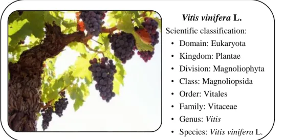
1 Vitis vinifera L. Scientific classification: • Domain: Eukaryota • Kingdom: Plantae • Division: Magnoliophyta • Class: Magnoliopsida • Order: Vitales • Family: Vitaceae • Genus: Vitis

• Species: Vitis vinifera L.

1. Introduction

1.1. The domesticated grapevine, Vitis vinifera L.

The members of the genus Vitis are collectively termed grapevines. This genus contains about 60 inter-fertile species which are native to the temperate and subtropical climate zones of the northern hemisphere, with a few species reaching the tropics (Vaughan and Geissler, 2009; Keller, 2015). Even though there are several species of grapevine only one of them, the Vitis

vinifera L. (Figure 1), originated in Eurasia, had a worldwide dispersion. This species has

become the world’s leading fruit crop, grown in almost 90 countries, mostly dedicated to the wine industry. However, it is also used in grape juice production, fresh table grape consumption and raisins (Bouquet, 2011; Keller, 2015).

Figure 1: Botanical classification of the domesticated grapevine (Keller, 2015).

The V. vinifera (2n=6x=38 chromosomes) was the fourth flowering plant and the first fruiting perennial crop whose genome was completely sequenced (Jaillon et al., 2007). The whole sequence progressed easily mainly because of its relatively low genome size, 487-500 million base pairs, that comprises proximally 30,000 genes (Jaillon et al., 2007; Velasco et al., 2007).

2 The V. vinifera shows considerable morphological variability and is a highly adaptable species, that can be grown in a very wide range of environments, even though it flourishes in Mediterranean like climates with warm dry summers and cool wet winters (Bouquet, 2011).

Some authors make a distinction between native wild vines of V. vinifera, referring to them as the subspecies V. vinifera ssp. silvestris, and domesticated species, designated subspecies V. vinifera ssp. sativa (also termed V. vinifera ssp. vinifera). This distinction is based on morphological differences that probably resulted from the domestication process of the plant (Vivier and Pretorius, 2000). The most noticeable difference is plant sex: wild grapevines are dioecious (presence of male and female plants), while cultivated forms are hermaphrodite. Also, domesticated grapes, in comparison to wild ones, have large elongated berries and seeds (vs small and round ones), more fruit per bunch and large leaves with entire or shallow sinuses (vs smaller, usually deep, three-lobed leaves) (Jackson, 2014).

The history and vineyard cultural practices have largely determined the genetic diversity that exists today in grapevines. The domestication of grapevine is closely linked to the discovery of wine, but it is unclear which process predated the other. Many archaeological findings suggest that these processes occurred 5,500-5,000 BC in southern Caucasia1_{, which} supports until now a large genetic diversity of wild grapes. Also, paleobotanical findings in Spain, dating 3,000 BC, raised the question about occurrence of a secondary domestication centre (Bouquet, 2011).

From the primo-domestication sites, there was a gradual spread to adjacent regions, such as Egypt and Lower Mesopotamia, and then further dispersal around the Mediterranean, following the main civilizations. Under the influence of Rome, grapevines extended throughout Europe and the Romans were the first to give name to grape varieties. In the middle ages, the Catholic Church replaced the Romans in spreading grapevine cultivation to new regions. By the end of the Middle Ages, wine drinking was a firmly established social custom in most of Europe, and viticulture grew steadily from the 16th to the 19th centuries, spreading across all the continents (This et al., 2006; Bouquet, 2011).

At the end of the 19th century, Europe suffered a Phylloxera plague that resulted in the devastation and destruction of many European vineyards, drastically decreasing the diversity of this species. European viticulture was saved from extinction by the introduction of several American Vitis species (disease resistant) that were used as rootstocks. Over the last 50 years,

3 the cultivated grapevine has undergone another drastic reduction of diversity, owing to the globalization of wine companies and markets, resulting in the emergence of the now familiar worldwide grown varieties such as Chardonnay, Cabernet Sauvignon, Syrah and Merlot, and the disappearance of old local varieties. Thus, the diversity V. vinifera has been shaped by human history through centuries (This et al., 2006).

Today, it’s estimated that proximally 10,000 grape varieties are being held in germplasm collections around the world (almost every winegrowing country has its own grapevine germplasm collection). But many varieties are known by several synonyms (different names for the same variety) or homonyms (identical name for different varieties). Therefore, This and colleagues (2006) estimated a more correct number of varieties of proximally 5,000, based on DNA profiling results, with many of them being closely related. In Portugal, there are 343 varieties that can be used in wine production, wherein 240 are thought to be autochthonous (Cunha et al., 2013).

The large diversity found within the species has been a result of mainly three processes which had a significant impact on the development and domestication of V. vinifera:

 Sexual reproduction - seeds seems to have had an important early role in the domestication and expansion of viticulture. Crossing probably occurred accidentally, due to pollen from proximate wild vines fertilizing cultivated vines (This et al., 2006; Jackson, 2014);

 Vegetative propagation by cuttings - this method allows maintaining and multiplying a highly desirable genotype so that a vineyard can be planted with a single variety. Cuttings are also a convenient method of transporting varieties from one region to another. Most of the world’s current vineyards are planted with varieties that have been perpetuated for centuries by vegetative propagation (This et al., 2006);

 Somatic mutations - in grapevine, natural mutations at the gene level are relatively frequent. Although vegetative propagation should ensure that all plants grown from cuttings have the same genotype, the occurrence of a somatic mutation in one cutting and not others might eventually led to slightly different genotype and sometimes a different phenotype in the same variety (This et al., 2006). For instance, varieties with green/yellow fruit arose from the mutation of two neighbouring genes of an original dark fruited grapevine (Keller, 2015).

In 2014, the worldwide surface area of vineyards was estimated to be 7,573 Kha and the world grape production was estimated at 737 Mqx, from which 55% was used for wine production, estimated to be around 270 MhL, 35% consumed as table grapes, 8% processed into raisins and the rest for juice and intermediate products production. In this same year,

4 Portugal had 224 Kha dedicated to vineyards, being the 8th largest area in the world and the 4th in the European Union. In 2014, Portugal produced 6.2 MhL of wine and consumed 4 MhL, making the country the 11th world wine producer and the 12th world wine consumer (OIV, 2015).

Wine is produced by yeast fermentation of sugars in grape juice to produce alcohol (ethanol) and carbon dioxide. Wine primary ingredients are water (86.8 %) and ethanol (11.2 %) however, the basic flavour of wine depends on more 20 additional compounds. The subtle differences that distinguish wines from one another depend on an even larger number of compounds (Jackson, 2014).

1.2. Biosynthesis of anthocyanins in grapevine

1.2.1. Anthocyanins overview

Anthocyanins and its derivatives are the principal source of the red colour in wines, which is one of the most important characteristics of red wines. Anthocyanins are odourless and nearly flavourless but they can interact with some aroma substances and influence the flavour of the wine (He et al., 2010; He et al., 2012). The amount and composition of anthocyanins present in a red wine varies greatly depending on the variety, maturity index (OU maturation stages of grapes), vintage, region of cultivation and many other factors, but the typical concentrations of free anthocyanins in full-bodied young red wines are around 500 mg/L, although in some cases it can be higher than 2,000 mg/L (He et al., 2012). In recent years considerable attention has been focused on the potential human health benefits of anthocyanins and their derived compounds present in grapes and wines (Nassiri-Asl and Hosseinzadeh, 2009).

Anthocyanins, synthesized via the flavonoid pathway, are the most abundant and widespread of the flavonoid pigments (Figure 2). They absorb light at the longest wavelengths and contribute to the colours orange, pink, red, blue and purple in coloured grapes, their wines and other products (Schwinn and Davies, 2004; He et al., 2010). Anthocyanins have different biological functions in plant tissues, such as protection against solar exposure and UV radiation, pathogen attacks, oxidative damage and attack by free radicals. They are also capable of attracting animals for seed dispersal, ameliorating biotic and abiotic stress and modulating signalling cascades (Flamini et al., 2013).

5

Figure 2: The basic flavonoid skeleton. Flavonoids are polyphenolic compounds comprising 15 carbons, with two aromatic rings (called the A- and B-rings) connected by a three carbon bridge that usually forms a third ring (called the C-ring). Hydroxyl groups are usually present at the 4’-, 5’- and 7-positions. The degree of oxidation and substitution of the C-ring determines the various classes of flavonoids (Crozier et al., 2009).

Anthocyanins synthesis is common throughout the plant kingdom, and they can occur in almost all tissues of higher plants, including roots, stems, leaves, flowers, and fruits (He et al., 2012). In V. vinifera, anthocyanins are located only in the skin of red grapes, with the exception of a few varieties, referred to as teinturier (e.g., Alicante Bouschet and Gamay Fréaux), that also contain anthocyanins in their pulp (Cheynier, 2006).

Structurally, anthocyanins are glycosides and acylglycosides of anthocyanidins, which have the typical C6-C3-C6 flavonoid skeleton (Figure 2), with different number and position of hydroxyl and methoxyl substituent groups in the B ring of the molecule. In most plants, only O-glycosylation occurs, however C-glycosylation can also happen (Saito et al., 2003). Glucose is the most common sugar used in the glycosylation and more than one molecule can be attached (Schwinn and Davies, 2004). In most V. vinifera varieties the glucose molecules can only be linked to the anthocyanidins through glycosidic bonds at the C3 positions to form 3-O-monoglycoside anthocyanins (He et al., 2010). In addition, the glucose of some anthocyanins is acetylated with aromatic or aliphatic acids (such as acetyl, p-coumaroyl and caffeoyl). Acetylation increases the anthocyanins stability and solubility and intensifies their colour. However, not all of the red grape varieties can produce acetylated anthocyanins in their berry skin (e.g., Pinot Noir) and the amount of acylated anthocyanins is highly variable according to the grape variety (He et al., 2010). Thus, anthocyanins have numerous possible structures in nature, and the anthocyanin profile for any kind of plant is distinctive.

In 2010, more than 600 different individual anthocyanins had already been identified from different plants, and this number is still increasing (He et al., 2010). In V. vinifera the main

6 monomeric anthocyanins (Figure 3) are pelargonidin-3-O-glucoside (callistephin),

cyanidin-3-O-glucoside (kuromanin), delphinidin-3-cyanidin-3-O-glucoside (myrtillin), peonidin-3-cyanidin-3-O-glucoside

(peonin), petunidin-3-O-glucoside (petunin) and malvidin-3-O-glucoside (oenin) (Flamini et al., 2013).

Figure 3: Structures of the principal V. vinifera anthocyanins (adapted from Flamini et al., 2013).

1.2.2. Anthocyanin biosynthesis pathway

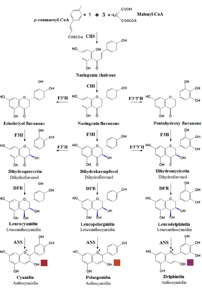
Anthocyanins are synthesized along the flavonoid pathway by the activity of a cytosolic multienzyme complex associated to the cytoplasmic surface of the endoplasmic reticulum (Braidot et al., 2008). The pathway can be divided into two parts, the basic flavonoid upstream pathway (Figure 4) and the specific anthocyanin downstream branch (Figure 5) (He et al., 2010).

The first step of the basic flavonoid upstream pathway (Figure 4) is the formation of the flavonoid C15 backbone by chalcone synthase (CHS). CHS carries out a series of sequential decarboxylation and condensation reactions, using one molecule of p-coumaroyl-CoA with three molecules of malonyl-CoA, to produce a naringenin chalcone. The A-ring is formed during this reaction. Then, in a reaction that establishes the flavonoid C-ring, chalcone isomerase (CHI; a.k.a. chalcone-flavanone isomerase) catalyses the stereospecific isomerization of the naringenin chalcone to its corresponding isomer naringenin (2S)-flavanone (Davies and Schwinn, 2006).

7

Figure 4: The basic upstream flavonoid pathway, ending in the biosynthesis of coloured anthocyanidins in V.

8 By the action of flavonoid 3’-hydroxylase (F3’H) or flavonoid 3’5’-hydroxylase (F3’5’H), the B ring of the naringenin flavanone can be further hydroxylated to produce eriodictyol or pentahydroxy-flavanone, respectively. All three (2S)-flavanones (naringenin, eriodictyol and pentahydroxy-flavanone) are converted stereospecifically to the respective (2R, 3R)-dihydroflavonols (dihydrokaempferol, dihydroquercetin and dihydromyricetin, respectively) through a hydroxylation in the C-ring that is catalysed by flavanone 3β- hydroxylase (F3H; a.k.a. FHT) (Figure 4). F3H is a soluble nonheme dioxygenase dependent on Fe2+, O2, and belongs to the family of oxoglutarate-dependent dioxygenase (ODD). 2-ODDs have been characterized from bacteria, fungi, vertebrate and plant sources, and they all use four electrons generated from 2-oxoglutarate decarboxylation to split di-oxygen and create reactive enzyme–iron species. 2-ODDs have eight amino acid residues that are strictly conserved in all species (Davies and Schwinn, 2006; Martens et al., 2010).

Furthermore, dihydrokaempferol is also a potential substrate for F3’H and F3’5’H, to produce the corresponding dihydroflavonols, dihydroquercetin and dihydromyricetin (Schwinn and Davies, 2004; He et al., 2010).

After these modifications, dihydroflavonol 4-reductase (DFR) reduces these three dihydroflavonols to their corresponding leucoanthocyanidins. The colourless leucoanthocyanidins are converted into the corresponding coloured anthocyanidins by the action of an anthocyanidin synthase (ANS; a.k.a. leucoanthocyanidin dioxygenase, LDOX) (Figure 4) (Grotewold, 2006; He et al., 2010).

Because anthocyanidins are unstable and generally do not accumulate in plants in the free state, they are converted to their corresponding stable anthocyanins by UDP-glucose: anthocyanidin: flavonoid glucosyltransferase (UFGT; a.k.a. F3GT, UF3GT, or 3GT). UFGT catalyzes the O-glycosylation of anthocyanidins through the addition of a glucose molecule at the C3 position (Figure 5) (Schwinn and Davies, 2004; He et al., 2010). Finally, anthocyanins can be further modified by methylation and/or acetylation. O-methyltransferase (OMT; a.k.a. anthocyanin O-methyltransferase, AOMT), with the participation of S-adenosyl-L-methionine (SAM), can mediate the methylation of the hydroxyl groups at the B-ring of the anthocyanins. The acylation of anthocyanins is catalysed by a group of enzymes collectively known as anthocyanin acyltransferases (ACT; a.k.a. AAT), which have really high substrate specificity, for both the anthocyanin acceptors and the acyl group donors (Figure 5) (He et al., 2010).

9

Figure 5: The specific anthocyanin downstream branch of the flavonoid pathway (adapted from He et al., 2010).

After synthesis in the cytosol, anthocyanins are delivered to a vacuole, where they are stored as coloured coalescences called anthocyanic vacuolar inclusions (Flamini et al., 2013).

As shown above, anthocyanins are synthesized by an extremely complex network of all the structural enzymes in the pathway. Different varieties present differences in the proportion of anthocyanins present in grapes mostly due to the particular pattern of expression of the whole set of genes involved in the biosynthesis (He et al., 2010).

10

1.3. Single Nucleotide Polymorphism genotyping

technologies

1.3.1. Single nucleotide polymorphism overview

Single Nucleotide Polymorphisms (SNPs) are changes in a single base at a specific position in the genome, found in more than 1% of the population (Kim and Misra, 2007; Bayés and Gut, 2011). As nucleotides are the smallest unit of inheritance, SNPs represent the most basic and abundant form of genetic sequence variation. Theoretically, a SNP can involve any of the four different nucleotide variants, but in practice they are generally biallelic and the different variants occur at different frequencies (Studer and Kölliker, 2013).

Mutation mechanisms can lead to the formation of SNPs by either: (1) a nucleotide transition, a purine is changed to a different purine (A ⇔ G) or a pyrimidine is changed to a different pyrimidine (C ⇔ T) or; (2) a nucleotide transversion, a purine is changed into a pyrimidine or vice-versa (A ⇔ C, A ⇔ T, G ⇔ C, G ⇔ T) (Vignal et al., 2002).

SNPs are not evenly distributed across the genome and occur at lower frequency in coding regions when compared to noncoding or intergenic regions (Studer and Kölliker, 2013). Depending on where a SNP occurs, it might have different consequences at the phenotypic level (Syvanen, 2001). In coding sequences, SNPs can cause alterations in protein structure and hence function, and in regulatory sites of a gene, SNPs can affect rates of transcription causing changes in the production of the encoded protein. However, SNPs are often synonymous and, thus, cause no changes. SNPs in noncoding regions do not alter encoded proteins, but can be used as genetic markers for comparative, evolutionary and genetic population studies (Kim and Misra, 2007).

SNP genotyping refers to the process of assigning the SNP variant to one of the four nucleotides, thereby discriminating alleles at a particular locus (Studer and Kölliker, 2013). As markers, SNPs possess important characteristics: they are highly abundant in genomes, have a low mutation rate which makes them stable and are co-dominant (Syvanen, 2001; Bayés and Gut, 2011). SNP genotyping has currently many applications in numerous fields such as genetic linkage analysis and trait mapping, diversity analysis, association studies and single marker or genome-wide marker assisted selection (Studer and Kölliker, 2013).

A variety of methods have been used to discover SNPs and many are available as commercial kits (Garvin et al., 2010). One SNP genotyping method can’t possibly fulfil the

11 requirements of every study that might be carried out. The choice of a method depends primarily on the scale of the genotyping project and the resources available. Generally, each method can be separated into two elements: (1) the biochemical method for discriminating SNP alleles and ; (2) the analysis/measurement of the allele specific products. SNP genotyping methods are still being improved (Bayés and Gut, 2011). Key targets are lowering the cost and increasing the simplicity, level of throughput and accuracy of the methods (Syvanen, 2001).

1.3.2. Allele discrimination strategies

Allele discrimination is mostly done with allele-specific biochemical reactions where primer extension, hybridization, ligation, and enzymatic cleavage are the most popular methods. Allele discrimination can also be done base on the physical properties of the DNA (Kim and Misra, 2007). Most of these strategies require a PCR amplification step to increase the number of target DNA molecules containing SNPs and to reduce the complexity of the template material used (Bayés and Gut, 2011).

1.3.2.1. Primer extension

Primer extension for allele discrimination is a technique based on the high accuracy of DNA polymerase to incorporate nucleotides complementary to the sequence of the template DNA during primer extension reaction. This tactic is very flexible, requires a small number of primers/probe and optimization is usually very straightforward (Kwok, 2001). Primer extension can be divided into two main approaches: a common primer for detecting both alleles or specific primers for detecting each allele (Kim and Misra, 2007).

The allele specific primer extension approach involves PCR amplification of genomic DNA using two forward allele-specific primers that are identical except for a mismatch at their 3’ end, where a SNP is known to exist, and a common reverse primer. Only the primer whose 3’ end perfectly matches the SNP will be extended by the DNA polymerase. The PCR fragments are separated on agarose-based electrophoresis gels and identified by fluorescence, allowing allelic discrimination (Figure 6) (Kim and Misra, 2007). This method is extremely simple. It can be used in any molecular biology laboratory and it also has been adapted to different genotyping techniques (Table 1). However, it is also very low-throughput and vulnerable to false negatives, since PCR failures cannot be reliably distinguished from genuine primer-binding discrimination in the absence of a reciprocal test. Considering the advantages and

12 disadvantages this method is best suited for the analysis of a limited number of SNPs in large sample collections (Syvanen, 2001; Chagné et al., 2007).

Figure 6: Primer extension approaches for SNP genotyping, specific primer extension reaction (adapted from Kim and Misra, 2007).

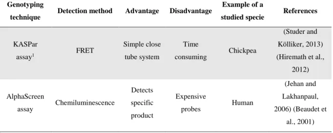
Table 1: Features of SNP-genotyping methods based in the specific primer extension approach.

Genotyping

technique Detection method Advantage Disadvantage

Example of a

studied specie References

KASPar assay1 FRET Simple close tube system Time consuming Chickpea (Studer and Kölliker, 2013) (Hiremath et al., 2012) AlphaScreen assay Chemiluminescence Detects specific product Expensive probes Human (Jehan and Lakhanpaul, 2006) (Beaudet et al., 2001) 1_{K-Biosciences}

In common primer extension reaction (Figure 7), a primer is designed to anneal with its 3’ end positioned on the base just preceding the SNP to be tested and is extended with ddNTPs by DNA polymerase. The identity of the extended base is determined either by fluorescence or mass to reveal SNP genotype (Kim and Misra, 2007). It is possible to detect up to four allelic variants for a variable site, discriminate heterozygous from homozygous genotypes and detect multiple SNPs simultaneously (Chagné et al., 2007). This approach serves as base to most sequencing technologies and some other genotyping techniques (Table 2).

13

Table 2: Features of SNP-genotyping methods based in the common primer extension approach.

Genotyping technique

Detection

method Advantage Disadvantage

Example of a

studied specie References

SNuPE1 _and SNaPshot2 systems Capillary electrophoresis DNA quantity and quality requirements are low Expensive equipment Japanese black pine and Arabidopsis (Chagné et al., 2007) (Suharyanto and Shiraishi, 2011) (Torjek et al., 2003) iPlex Gold MassARRAY3 MALDI-TOF MS

Low cost per data point and

medium to high throughput Expensive equipment Maize (Studer and Kölliker, 2013) (Ragoussis, 2009) (Jones et al., 2007)

GOOD assay MALDI mass

spectrometry No labelling method Multi-step procedure Bovine and Human

(Kim and Misra, 2007) (Sauer et al., 2000) (Sauer et al.,

2002)

1_{GE Healthcare;} 2_{Applied Biosystems;} 3_Sequenom

Figure 7: Primer extension approaches for SNP genotyping, common primer extension reaction. (a) Extension products are detected by mass spectrometry and the difference between mass of extension product and primer identifies incorporated nucleotide(s) and hence the SNP genotype. (b) This technique uses ddNTPs that are labelled with different fluorescent tags. Products are detected by fluorescence after capillary electrophoresis and the colour of the dye indicates incorporated base(s) and hence the SNP genotype (adapted from Kim and Misra, 2007).

14 1.3.2.1.1. Sequencing

Sequencing genomes can be used to potentially identify millions of genome-wide SNPs, allowing the characterization of genes and genomes, and providing a more comprehensive view of diversity and gene function (Deschamps et al., 2012). Direct sequencing of PCR products is now widely used for SNP genotyping candidate genes. Also, sequencing data is often used as a benchmark standard in studies for the evaluation of novel SNP genotyping methods (Chagné et al., 2007). This is possible due to the increased ability to sequence in a cost-effective manner large numbers of individuals within the same species. In the past thirty years, DNA sequencing technologies and applications have undergone tremendous development and act as the engine of the genome era (Liu et al., 2012). Here, the main sequencing technologies will be briefly presented, starting by the classic Sanger sequencing method and ending in the most modern technologies currently available.

In 1977, Frederick Sanger and colleagues developed a enzymatic dideoxy DNA sequencing technology (Sanger et al., 1977). This sequencing method takes advantage of the ability of DNA polymerase to incorporate 2′,3′-dideoxynucleotides (ddNTPs), nucleotide base analogues that lack the 3′-hydroxyl group essential in phosphodiester bond formation, which leads to chain termination (Applied Biosystems, 2009). Due to its high efficiency this method was adopted as the primary technology in the “first-generation” sequencing methods (Liu et al., 2012). Since its development, Sanger sequencing has gone through several improvements, including automated sequencers, and it’s still the gold standard for generating high quality sequencing information (Deschamps et al., 2012).

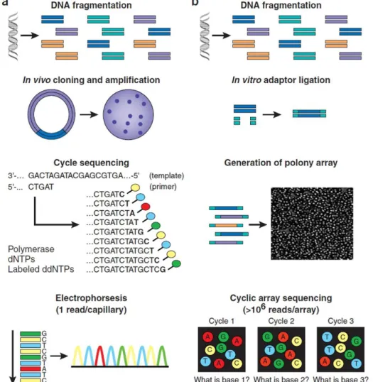
In the current Sanger sequencing method (Figure 8a) the DNA that is going to be sequenced is first amplified. For high-throughput shotgun de novo sequencing the genomic DNA is fragmented, cloned into a plasmid vector, then Escherichia coli is used for transformation and for each sequencing reaction a single bacterial colony is picked. For a specific DNA fragment resequencing, PCR amplification is carried out with primers that flank the target DNA. The sequencing biochemistry takes place in a “cycle sequencing” reaction, in which successive rounds of template denaturation, primer annealing and primer extension are performed (Shendure and Ji, 2008). Each round of primer extension is terminated by the incorporation of a fluorescently labelled ddNTPs. In the end of the “cycle sequencing” reaction, there will be a mixture of different size extension products labelled in their 3’ end. These fragments are then separated by size via capillary electrophoresis. During the separation process the fluorescently labelled DNA fragments pass through a laser beam that makes the dyes on the

15 fragments fluoresce (each dye emits light at a different wavelength when excited, therefore all four bases can be detected). An optical detection device detects the fluorescence signal and a data collection software translates the fluorescence signal to digital DNA sequences (Applied Biosystems, 2009). The subsequent approach for data analysis, such as genome assembly or variant identification, depends on what is being sequenced and why (Shendure and Ji, 2008).

Figure 8: Workflow of (a) conventional versus (b) “second-generation” sequencing methods (Shendure and Ji, 2008).

The Sanger sequencing can achieve read-lengths of up to ≈1,000 bp, per-base “raw” accuracies as high as 99.999% and a time run up to 3 hours (Shendure and Ji, 2008). These are some of the reasons that justify the use of this technique in the first human genome sequencing program (Lander et al., 2001). Sanger sequencing was also used in several plant species whole genome sequencing projects, such as Arabidopsis thaliana L. (The Arabidopsis Genome Initiative, 2000), rice (Oryza sativa L.) (Goff et al., 2002), sorghum (Sorghum bicolor L.) (Paterson et al., 2009) and soybean (Glycine max L.) (Schmutz et al., 2010).

16 In 2007, V. vinifera was sequenced by two different groups: Jaillon and colleagues in September and Velasco and colleagues in October. The group of Jaillon and colleagues (2007) sequenced a grapevine line, originally derived from Pinot Noir that was bred close to full homozygosity (PN40024). They discovered that the grapevine genome has 41.4% repetitive/transposable elements and 30,434 protein-coding genes. The group of Velasco and colleagues (2007) sequenced the Pinot Noir clone ENTAV 115, a variety grown in a range of soils for the red and sparkling wine production. This group estimated that the genome size of

V. vinifera to be 504.6 Mb, with 29,585 genes. They were also able to map 1,751,176 SNPs.

Having a sequenced reference genome, in the grapevine case the Pinot Noir variety, allows high throughput resequencing of varieties or wild species to extend the current knowledge of the molecular basis of polymorphism (Adam-Blondon et al., 2011).

However, the Sanger sequencing is associated with high costs and labour which limits its reach and use in large and complex genomes. This limitations contributed to the emergence of “next-generation” sequencing technologies, the second- and third-generation (Deschamps et al., 2012). Currently, there are three top companies that commercialise sequencing platforms of “second-generation” technology: Roche, Illuminaand Life Technologies (see Table 3) (Pareek et al., 2011). Although these platforms are quite diverse in sequencing biochemistry as well as in how the array is generated, their workflows are conceptually similar (Figure 8b). Library preparation consists in the random fragmentation of DNA, followed by in vitro ligation of universal adaptor sequences. Then the PCR amplicons derived from any given single library molecule end up forming PCR colonies spatially clustered and immobilized, either to a single location on a planar substrate (Illumina platforms), or to the surface of micron-scale beads, which can be recovered and arrayed (Roche and Life Technologies platforms). Each PCR colony consists of many copies of a single shotgun library fragment. The sequencing process itself consists on sequencing by synthesis, which is the serial extension of primed templates where the enzyme driving the synthesis can be either a polymerase (Roche and Illumina platforms) or a ligase (Life Technologies platform) (Shendure and Ji, 2008). The incorporation of one or more labelled nucleotides is followed by the emission of a signal that is detected by the sequencer (Deschamps et al., 2012). In these platforms a single microliter-scale reagent volume can be applied to manipulate all the arrays features in parallel. Also, data is acquired by imaging the full array at each cycle (Shendure and Ji, 2008).

17

Table 3: Comparison of different “second-generation” sequencing platforms. Features of different massively parallel sequencing technologies have been compiled from the websites of the respective companies (adapted from Thudi et al., 2012).

Company Sequencer Throughput Read length Accuracy Run time

Roche/454 sequencing GS-FLX 454 Junior System ≈35 Mb ≈400 bp 99 10 h GS FLX Titanium XLþ 700 Mb Up to 1,000 bp 99.997 23 h GS FLX Titanium XLR70 450 Mb Up to 600 bp 99.995 10 h Illumina/ SOLEXA HiSeq 2000 Up to 600 Gb 2x100 bp >85 (2x50 bp); >80 (2x100 bp) 1.5 - 11 days HiSeq 1000 Up to 300 Gb 2x100 bp >85 (2x50 bp); >80 (2x100 bp) 1.5 - 8.5 days Genome Analyzer IIx 95 Gb 2x150 bp >85 (2x50 bp); >80 (2x100 bp) 2 - 14 days MiSeq >1 Gb 2x150 bp >85 (2x50 bp); >80 (2x100 bp) 8 h Life

Technologies 5500 System 7-9 Gb/day

Mate-paired: 2x60 bp; Paired-end: 75 bp x 35 bp; Fragment: 75 bp Up to 99.99 2 - 8 days SOLiD™ 4 System Up to 100 Gb Mate-paired: 2x35 bp; 2x50 bp; Paired-end: 50 bp x 25 bp; Fragment: 50 bp 99.94 3.5 – 16 days

These “second-generation” platforms present some advantages when compared to the Sanger sequencing method: they allow a much higher degree of parallel analysis, high throughput, have a considerable reduced cost, fewer infrastructure requirements and allow real time sequencing (Shendure and Ji, 2008; Liu et al., 2012). They also have theirs disadvantages:

18 a higher error rate than traditional Sanger sequencing, shorter reads, which difficult the data management, and data generation is more time consuming (Deschamps et al., 2012; Thudi et al., 2012). Although these limitations create important challenges for the immediate future, these technologies will continue to be improved, like conventional sequencing was until it reached its current level of technical performance (Shendure and Ji, 2008).

In the recent years a “third-generation” of sequencing platforms have been emerging. These new platforms do not require PCR amplification prior to sequencing, as opposed to second-generation ones (Liu et al., 2012). Theoretically, the third-generation sequencing platforms are able to sequence from single molecules of DNA and are capable of direct RNA sequencing. Although the PCR amplification has revolutionized DNA analysis, in some instances, it may introduce base sequence errors or favour certain sequences over others, thus changing the relative frequency and abundance of the various DNA fragments that existed before amplification. When compared to “second-generation” sequencing these new platforms present some advantages: higher throughput, faster turnaround time, longer read lengths, higher accuracy, smaller amounts of starting material and lower cost (Pareek et al., 2011). As it can be seen in Table 4, there are already several “third-generation” sequencing platforms.

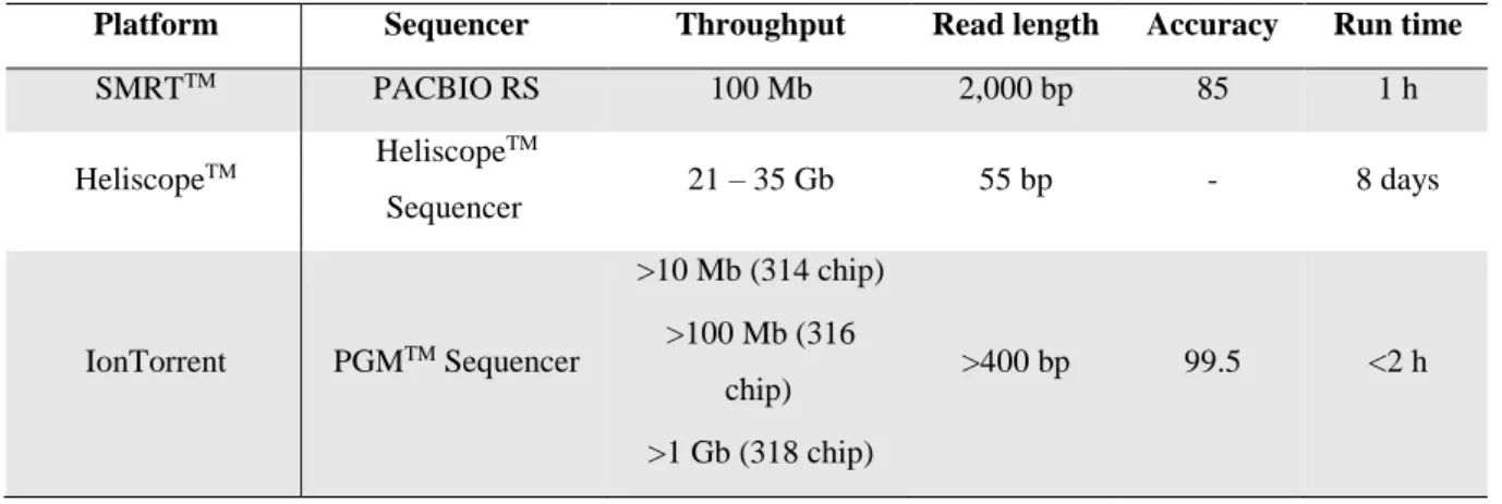
Table 4: Comparison of different “third-generation” sequencing platforms. Features of different sequencing platforms have been compiled from the websites of the respective companies (adapted from Thudi et al., 2012).

Platform Sequencer Throughput Read length Accuracy Run time

SMRTTM _{PACBIO RS 100 Mb 2,000 bp 85 1 h} HeliscopeTM Heliscope TM Sequencer 21 – 35 Gb 55 bp - 8 days IonTorrent PGMTM _Sequencer >10 Mb (314 chip) >100 Mb (316 chip) >1 Gb (318 chip) >400 bp 99.5 <2 h

In the past several years “next-generation” sequencing have been applied for a variety of important applications, including: full-genome resequencing, targeted discovery of mutations and polymorphisms, mapping structural rearrangements, RNA sequencing, detection of methylated regions in genome and genome-wide mapping of DNA-protein interactions. Over the next few years, the list of applications will undoubtedly grow, as will the sophistication with which existing applications are carried out (Pareek et al., 2011; Thudi et al., 2012).

19

1.3.2.2. Hybridization

Hybridization approaches use differences in thermal stability of double-stranded DNA to distinguish between perfectly matched and mismatched target-probe pairs for achieving allelic discrimination. Under optimized assay conditions, a one base mismatch is sufficient to destabilize the hybridization between an allelic specific probe and its target sequence (Kwok, 2001; Kim and Misra, 2007). However, it is difficult to predict the ideal reaction conditions or the sequence of the probe that will allow the optimal distinction between two alleles that differ at a single nucleotide position. These parameters must be established empirically and individually for each SNP. Considering the thermal stability of the hybrid target-probe, it is determined by several parameters, such as: the stringency of the reaction conditions, the nucleotide sequence that flanks the SNP, the secondary structure of the target sequence, the SNP position in the probe (usually located in a central position) and the probe length (Chagné et al., 2007; Kim and Misra, 2007). In hybridization assays the allele specific probes can be immobilized on a solid support or they can be used in a homogeneous reaction (Kwok and Chen, 2003). Some of the genotyping techniques that are based on hybridization are summarized in the Table 5.

20

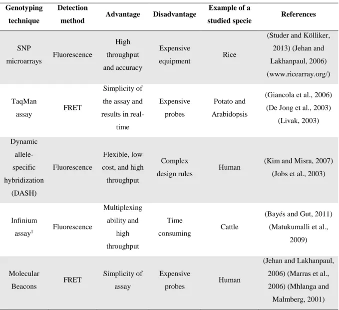
Table 5: Features of SNP-genotyping methods based in hybridization.

Genotyping technique

Detection

method Advantage Disadvantage

Example of a

studied specie References

SNP microarrays Fluorescence High throughput and accuracy Expensive equipment Rice

(Studer and Kölliker, 2013) (Jehan and Lakhanpaul, 2006) (www.ricearray.org/) TaqMan assay FRET Simplicity of the assay and results in real-time Expensive probes Potato and Arabidopsis (Giancola et al., 2006) (De Jong et al., 2003)

(Livak, 2003) Dynamic allele-specific hybridization (DASH) Fluorescence Flexible, low cost, and high throughput

Complex

design rules Human

(Kim and Misra, 2007) (Jobs et al., 2003) Infinium assay1 Fluorescence Multiplexing ability and high throughput Time consuming Cattle

(Bayés and Gut, 2011) (Matukumalli et al., 2009) Molecular Beacons FRET Simplicity of assay Expensive probes Human

(Jehan and Lakhanpaul, 2006) (Marras et al., 2006) (Mhlanga and Malmberg, 2001)

1_Illumina

1.3.2.3. Ligation

Ligation approaches (Table 6) rely on the specificity of DNA ligases to repair DNA nicks. Generally, three oligonucleotide probes are used: two are allele specific and bind to the template DNA at the SNP site, and the third is a common probe that binds to the template DNA immediately next to the allele-specific probe. When the allele specific and common probes hybridize to single stranded template DNA with perfect complementarity, adjacent to each other, ligase enzymes joins them to form a single oligonucleotide. Usually, the SNP site in the allele-specific probes is located at their 3’ ends because ligases are more sensitive to mismatches in that position. The ligation products are then detected by various ways, like fluorescence or gel electrophoresis, allowing allelic discrimination (Kim and Misra, 2007;

21 Bayés and Gut, 2011). Ligation methods have high specificity, are easy to optimize and can genotype without prior target amplification by PCR. However, compared primer extension methods, it requires more oligonucleotides, which obviously increases the costs of these assays (Kwok, 2001; Syvanen, 2001).

Table 6: Features of SNP-genotyping methods based in ligation.

Genotyping technique

Detection

method Advantage Disadvantage

Example of a

studied specie References

Molecular inversion probes (MIP) assay1 Fluorescence Multiplexing ability and high throughput Expensive hardware Human (Ragoussis, 2009) (Syvanen, 2005) (Hardenbol et al., 2005) GoldenGate assay2 Fluorescence Multiplexing ability and high throughput Expensive hardware Apple, maize, soybean and wheat (Khan et al., 2011) (Yan et al., 2010) (Akhunov et al., 2009) (Hyten et al., 2008) SNPlex system3 Capillary electrophoresis and fluorescence Multiplexing ability and low DNA consumption Time consuming (2 days to complete) Grapevine (Pindo et al., 2008) (Vezzulli et al., 2008)

(De la Vega et al., 2005) (Tobler et al., 2005) Padlock probes Fluorescence Localized detection Probes difficult to produce Wheat (Edwards et al., 2009) (Jehan and Lakhanpaul, 2006)

1_Affymetrix; 2_Illumina; 3_{Applied Biosystems}

1.3.2.3. Enzymatic cleavage

Enzymatic cleavage is based on the ability of endonucleases enzymes to cleave DNA by recognition of specific sequences and/or structures. Allelic discrimination can be achieved when a SNP is located in the enzyme recognition sequence (Kim and Misra, 2007). In Table 7 are summarized some of the genotyping techniques based in this approach.

22

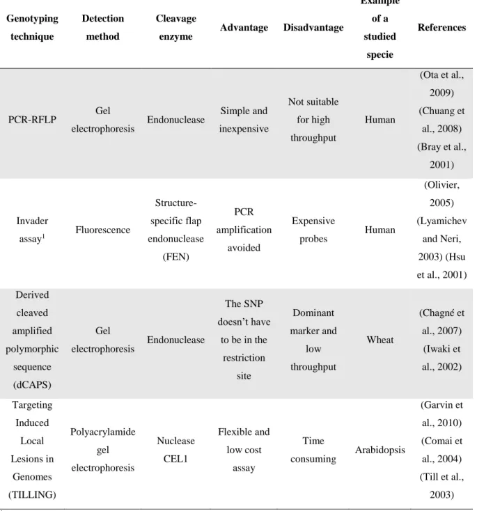
Table 7: Features of SNP-genotyping methods based in enzymatic cleavage.

Genotyping technique

Detection method

Cleavage

enzyme Advantage Disadvantage

Example of a studied specie References PCR-RFLP Gel electrophoresis Endonuclease Simple and inexpensive Not suitable for high throughput Human (Ota et al., 2009) (Chuang et al., 2008) (Bray et al., 2001) Invader assay1 Fluorescence Structure-specific flap endonuclease (FEN) PCR amplification avoided Expensive probes Human (Olivier, 2005) (Lyamichev and Neri, 2003) (Hsu et al., 2001) Derived cleaved amplified polymorphic sequence (dCAPS) Gel electrophoresis Endonuclease The SNP doesn’t have to be in the restriction site Dominant marker and low throughput Wheat (Chagné et al., 2007) (Iwaki et al., 2002) Targeting Induced Local Lesions in Genomes (TILLING) Polyacrylamide gel electrophoresis Nuclease CEL1 Flexible and low cost assay Time consuming Arabidopsis (Garvin et al., 2010) (Comai et al., 2004) (Till et al., 2003)

1_{Third wave technologies}

1.3.2.4. Physical properties of the DNA

The physical characteristics of DNA, i.e. the melting temperature and single strand conformation when placed in non-denaturing conditions, can be used for allele discrimination (Studer and Kölliker, 2013). High resolution melting (HRM) and some other genotyping techniques (Table 8) fit this category.

23

Table 8: Features of SNP-genotyping methods based in the physical properties of the DNA.

Genotyping technique

Detection

method Advantage Disadvantage

Example of a

studied specie References

Strand conformation polymorphism (SSCP) Capillary electrophoresis Simplicity of the assay Not suitable for high throughput Grapevine (Konstantinos et al., 2008) (Dong and Zhu, 2005) (Salmaso et al., 2004) Temperature Gradient Gel Electrophoresis (TGGE) Capillary electrophoresis No prior knowledge of the DNA sequence needed Time

consuming Maize (Hsia et al., 2005)

Denaturing High Pressure Liquid Chromatography (dHPLC) Chromatography No prior knowledge of the DNA sequence needed Time consuming and only detects the presence/ absence of the SNP Barley (Jehan and Lakhanpaul, 2006) (Kota et al., 2001)

1.3.2.4.1. High resolution melting curve analysis

High resolution melting (HRM) is a simple, PCR-based method, for detecting DNA sequence variation by measuring changes in the melting of a DNA duplex (Taylor, 2009). The melting temperature (Tm) of a DNA duplex is the temperature at which 50% of the DNA duplexes have dissociated and its characteristic of its GC content, length and sequence (Reed et al., 2007). For HRM analysis, duplexes may be formed from the two strands of a PCR amplicon or from an oligonucleotide probe and an amplicon strand (Taylor, 2009).

For HRM analysis, a PCR is carried in the presence of dyes that fluoresce when intercalated in double-stranded DNA. The PCR product is then heated through a range of temperatures while the level of fluorescence is measured (Reed et al., 2007; Taylor, 2009). Any double-stranded DNA will fluoresce strongly at low temperatures. As the temperature rises the fluorescence will decrease, at first slowly, and then, at the Tm, the fluorescence rapidly drops, reflecting the melting of DNA into single strands (as shown in Figure 9) (Reed et al., 2007). The fluorescence data generated during DNA melting can be analysed based on the Tm or on the shape of the melting curve. Accurate calculation of Tm first requires the mathematical

24 removal of background and normalization of the melting curve, which can be performed by commercial HRM software (Reed et al., 2007; Erali et al., 2008).

Figure 9: Normalized data showing the rapid fluorescence decrease around the Tm, when the DNA goes from

double-stranded to single stranded (adapted from Reed et al., 2007).

The sensitivity and specificity of HRM depends greatly on the dye, instrument, software used and purity of the PCR product (Erali and Wittwer, 2010). To obtain better results novel saturation dyes and high-resolution instruments were specifically developed for HRM. These new DNA binding dyes have improved saturation properties, which results in the PCR product being labelled along its entire length, so that all domains are detected. They also exhibit minimal redistribution during melting and do not inhibit PCR over a wide range of concentrations (Reed et al., 2007; Erali et al., 2008). In addition to saturation dyes, new instrumentations that allow high controlled temperature transitions and data acquisition were developed specifically for HRM analysis. Furthermore, some real-time thermal cyclers were modified to incorporate HRM even though they do not perform as well as instruments dedicated only to HRM. However, there is convenience in having both amplification and melting analysis combined in one instrument (Reed et al., 2007).

While genotyping PCR products by HRM, smaller amplicons allow a better discrimination of small sequence variations than bigger amplicons (Erali et al., 2008). When the amplicon is short melting occurs in one transition, without intermediate states. In contrast, longer amplicons melt in multiple stages or domains, with AT-rich regions melting at lower

25 temperatures than GC-rich regions. This results in bigger Tm differences among the genotypes in the shorter amplicons (Erali and Wittwer, 2010).

In SNP genotyping, heterozygotes are easy to identify because of the change in the melting curve shape. A heterozygous sample contains four duplex species (two heteroduplexes and two homoduplexes) and its observed melting curve is a sum of the four individual melting curves. Due to the contribution of the unstable heteroduplexes, the shape of the heterozygous melting curve changes, in comparison to the shape of the homozygous melting curve (Figure 10) (Taylor, 2009).

Figure 10: Single base genotyping by small amplicon melting. In this example an AC variation is showed, with the possible genotypes A/A, A/C and C/C represented. The A/A and C/C curves are similar in curve with the Tm

of the C/C homozygote approximately 1°C higher than the A/A homozygote. The A/C heterozygote melting curve differs in shape from that of the homozygotes, with a more gradual transition over a larger temperature range (adapted from Reed et al., 2007).

A homozygous sequence variant usually changes the Tm of the duplex, however not all homozygotes can be distinguished by Tm. When there is an exchange between G:C and T:A base pairs, the change in Tm is relatively large in small amplicons (approximately 0.8– 1.4 °C), as shown in Figure 10. If, however, the bases swap strands but the base-pair does not change, the change in Tm is smaller, becoming undetectable if there is also nearest-neighbour symmetry. In this case, a known homozygote is mixed into each unknown homozygote and the mixture is melted again (Reed et al., 2007; Vossen et al., 2009).

In addition, known sequence variants may be genotyped by HRM analysis using unlabelled oligonucleotide probes (Figure 11). These probes are included in the PCR master

26 mix which also contains asymmetric ratios of primers to generate one strand of DNA in excess (asymmetric PCR). Some of the excess strands hybridize to the complementary unlabelled probe. Both probe and amplicon duplexes will be saturated with dye (Reed et al., 2007; Erali et al., 2008). Because probe-amplicon duplexes melt at lower temperatures than amplicon duplexes, both products can be analysed from one melting curve.

Figure 11: Asymmetric PCR in the presence of an unlabelled probe. Excess primer (red) is complementary to strand A and produces excess copies of strand B. The limiting primer (blue) is complementary to strand B and produces limited copies of strand A. Excess copies of strand B increases visibility of the probe-amplicon duplex. HRM analysis shows both PCR product and unlabelled probe melting (adapted from Zhou et al., 2005; Montgomery et al., 2007).