Energy and Temperature Aware Real-Time Systems

(1)

F

ACULDADE DE

E

NGENHARIA DA

U

NIVERSIDADE DO

P

ORTO

Energy and Temperature Aware

Real-Time Systems

Muhammad Ali Awan

D

ISSERTATION

Doctoral Program in Electrical and Computer Engineering Supervisor: Stefan Markus Ernst Petters

(2)

(3)

Energy and Temperature Aware Real-Time Systems

Muhammad Ali Awan

Doctoral Program in Electrical and Computer Engineering

Approved by:

President: Dr. Jose Alfredo Ribeiro da Silva Matos External Referee: Dr. Gerhard Fohler

External Referee: Dr. Marko Bertogna

FEUP Referee: Dr. Luis Miguel Pinho Almeida FEUP Referee: Dr. Mario Jorge Rodrigues de Sousa Supervisor: Dr. Stefan Markus Ernst Petters

(4)

(5)

Abstract

Modern embedded systems have increasingly penetrated our daily life, and have facilitated and accelerated our regular activities. Some of these systems are constrained with strict timing re-quirements, and have limited and/or intermittent power supply. One of the major challenges in the design process of such systems is to minimise their energy consumption and thus to increase the battery life and enhance their mobility. In order to address this objective, it is important to understand the current trends in the embedded systems industry. With progressing CMOS tech-nology miniaturisation, the leakage power dissipation — once neglected — has become a major contributor to the overall power dissipation of modern embedded systems and as a matter of fact it has started to dominate its counterpart, the dynamic power dissipation. To cope with current trend of increasing leakage current, hardware vendors have equipped modern embedded processors with several sleep states and reduced the overhead (energy/time) of a sleep transition. Secondly, there is a trend towards an increased number of devices, as an ever increasing need for extra functionality in a single embedded system demands for extra Input/Output (I/O) devices, which are expensive in terms of energy consumption. Similar to processors, these devices are also equipped with low power sleep states to reduce their energy consumption. Thirdly, modern embedded processors have started to suffer from thermal issues due to increase in power density. It is essential to keep the temperature within recommended limits for the safe operation of the system and to increase the durability/reliability of hardware platforms. Finally, the CMOS industry experienced a paradigm shift in the last decade from single processor design to multicore hardware platforms as the clock frequency cannot be further increased efficiently to enhance the performance of the system. This is driven by the increase in performance per watt ratio that demands special packaging techniques to dissipate the generated heat at high frequencies.

This dissertation attempts to provide energy efficient solutions and techniques to cope with the aforementioned arising trends, while closing the gap between theoretical research and practice. In particular, it focuses at the operating-system-level power management and exploits the available sleep states to improve on energy efficiency while mainly concentrating on the leakage power dissipation. Uniprocessor power management has been widely explored in the last two decades. Several procrastination approaches has been proposed in the literature to deal with the leakage current. However, these solutions approximate the procrastination interval to ease the analysis and sub-optimally utilise the available resources to minimise energy consumption. Such approx-imation is eliminated in this dissertation with the optimal algorithm to maximise energy savings. A practical limitation of the procrastination scheduling algorithm is relaxed by eliminating the need for an external hardware to implement the power saving algorithm. These newly developed algorithms with low complexity save energy comparable to procrastination scheduling. Further-more, this dissertation demonstrates that idealised dynamic voltage and frequency scaling, and the thermally constrained dynamic power management are equivalent in nature. Hence, existing solu-tions proposed for dynamic voltage and frequency scaling can be easily ported to increase energy efficiency in thermally constrained systems.

(6)

Intra-task I/O device scheduling was vastly ignored in the past due to an increased overhead of sleep transitions. A decrease in sleep transition overheads allows to explore this new paradigm of device scheduling. This solution not only minimises the pessimism involved in traditional device scheduling algorithms but also reduces the online overhead of scheduling algorithms and has the flexibility to scale easily with an increase in I/O devices. Finally, this dissertation addresses the power management in the context of multicore hardware platforms. Global scheduling algorithms have become an attractive choice to schedule applications on a homogeneous multicore platform. The proposed energy saving algorithm exploits the spare capacity in the schedule and exploits the sleep states available in homogeneous multicore platform to save energy consumption. Heteroge-neous multicore platforms are famous in modern computing to perform specific tasks efficiently. Energy efficient mapping on heterogeneous multicore platforms addressed in the literature consid-ers only dynamic power dissipation while assuming leakage power dissipation a constant factor. Opposed to the state-of-the-art, the proposed allocation heuristics in the thesis are divided into two phases to tackle both dynamic and leakage power dissipation. All the algorithms proposed in this dissertation are evaluated with extensive set of simulations for a variety of hardware platforms and workloads.

(7)

Resumo

É um facto constatado que os sistemas embebidos têm tomado um lugar relevante na nossa vida quotidiana, tendo facilitado e até acelerado as nossas actividades diárias. Alguns destes sistemas caracterizam-se por requisitos temporais bastante rigorosos e são alimentados por fontes de en-ergia limitadas e/ou intermitentes. Um dos maiores desafios no projecto deste tipo de sistemas consiste em minimizar o seu consumo de energia e, consequentemente, aumentar a sua autono-mia e mobilidade. De forma a atingir este objectivo, é fundamental compreender as tendências actuais na indústria dos sistemas embebidos. Com a progressiva miniaturização da tecnologia CMOS, a potência devida à corrente de fuga – anteriormente desprezável – tornou-se numa das principais contribuições para o total da potência dissipada. Na realidade, a potência da corrente de fuga consegue já ultrapassar em certos casos aquela que era a principal fonte de dissipação de potência nos circuitos CMOS: a potência dinâmica, associada à transição entre estados. Para lidar com esta crescente potência da corrente de fuga, os fabricantes de circuitos equiparam os actu-ais processadores embebidos com vários estados de latência (sleep modes) e reduziram os custos energéticos e temporais associados a uma transição por um estado latente. Adicionalmente, há a tendência de se aumentar o número de dispositivos incluídos num único sistema embebido, dev-ido à crescente complexidade da funcionalidade exigida às aplicações embebidas, requerendo um maior número de dispositivos de entrada-saída (I/O), traduzindo-se na prática por um aumento do consumo energético. Tal como no caso dos processadores, estes dispositivos também estão equipa-dos com estaequipa-dos de latência, de forma a reduzir o consumo de energia. Um outro ponto a ter em conta relaciona-se com os problemas térmicos, devidos ao aumento da densidade de potência, presentes nos actuais processadores embebidos. É fundamental manter a temperatura dentro dos limites especificados para a operação segura do sistema e aumentar da durabilidade/fiabilidade da plataforma computacional. Por último, o paradigma de fabrico CMOS evoluiu na última década, do projecto de sistemas com um único processador para plataformas com múltiplos núcleos de ex-ecução (multi-core), pois tornou-se impossível continuar a obter ganhos de desempenho através do aumento da frequência de relógio. Esta mudança é motivada pelo aumento da relação de desem-penho por watt, através de técnicas especiais de desenho dos circuitos integrados que permitem dissipar o calor gerado a altas-frequências.

Esta dissertação apresenta um conjunto de novas soluções eficientes do ponto de vista en-ergético para lidar com as tendências previamente referidas, estabelecendo simultaneamente a ponte entre a investigação teórica e a prática. Este trabalho centra-se em particular na gestão de energia ao nível do sistema operativo, e explora os estados de latência disponíveis para melhorar a eficiência energética, concentrando-se na dissipação de potência devida às correntes de fuga. A gestão de energia em sistemas uniprocessador foi largamente explorada nas últimas duas décadas. Neste período, publicaram-se várias abordagens baseadas na procrastinação de tarefas para lidar com o problema da corrente de fuga. No entanto, estas soluções estimam um valor aproximado do intervalo de procrastinação para facilitar a análise e utilizar de forma sub-óptima os recursos disponíveis para minimizar o consumo de energia. Este trabalho conseguiu eliminar a referida

(8)

aproximação com um algoritmo óptimo para maximização da poupança de energia. A limitação prática do algoritmo de escalonamento com procrastinação de tarefas é relaxado através da elim-inação da utilização de hardware externo para implementar o algoritmo de poupança de energia. Estes novos algoritmos de baixa complexidade, desenvolvidos neste trabalho, atingem poupanças de energia comparáveis ao escalonamento com procrastinação de tarefas. Além disso, esta disser-tação demonstra como a variação dinâmica ideal de tensão e frequência, e a gestão dinâmica de consumo de potência baseada em factores térmicos são, por natureza, equivalentes. Desta forma, as actuais soluções propostas para variação dinâmica de tensão e frequência podem ser facilmente convertidas para aumentar a eficiência energética em sistemas com restrições térmicas.

O escalonamento de dispositivos de entrada-saída ao nível da tarefa tem sido negligenciado devido aos custos elevados de transições por estados de latência. A diminuição desses custos permite explorar este novo paradigma de escalonamento de dispositivos. Esta solução não só minimiza o pessimismo relacionado com os algoritmos tradicionais de escalonamento de dispos-itivos como também reduz os custos de execução dos algoritmos de escalonamento, possuindo a flexibilidade necessária para facilmente acompanhar um número crescente de dispositivos de entrada-saída. Por fim, esta dissertação aborda a gestão de potência no contexto das plataformas baseadas em arquitecturas de processadores com múltiplos núcleos de execução (multi-core). Os algoritmos de escalonamento globais tornaram-se uma opção interessante para ordenar a execução de tarefas em plataformas cujos múltiplos são homogéneos. O algoritmo para poupança de ener-gia proposto, explora a capacidade excedente do sistema decorrente do escalonamento, bem como os estados de latência disponíveis nestas plataformas de núcleos homogéneos, afim de reduzir o consumo de energia. As plataformas de núcleos heterogéneos são reconhecidas pela capacidade de realizar eficientemente tarefas específicas. Os processos de afectação de tarefas por núcleos de execução baseada em critérios de eficiência energética publicados até hoje, consideram apenas a dissipação dinâmica de potência assumindo um factor constante para a potência devida à cor-rente de fuga. Em oposição ao estado-da-arte actual, as heurísticas de afectação proposta nesta dissertação dividem-se em duas fases para abordar tanto a dissipação de potência dinâmica como a dissipação de potência de fuga. Todos os algoritmos propostos nesta dissertação são avaliados através de um extenso conjunto de simulações para uma variedade de plataformas computacionais submetidas a diversas cargas.

(9)

Acknowledgements

A PhD milestone demands dedication, hard work, patience, concentration, motivation and support from people around you. Many individuals made this challenging milestone easier for me and paved the way to my success. First of all, I would like to express my very great appreciation and gratitude to my supervisor Stefan M. Petters for his valuable ideas, constructive discussions, useful feedback and excellent guidance. He never let me down at any stage and kept my motivation alive throughout my PhD process. I am very grateful to him for providing me such an exciting opportu-nity to work on this interesting topic, sharing his vast experience in this domain and encouraging me to work on different problems of my choice within this topic. I have learned a lot during his extraordinary supervision. I would also like to thank Eduardo Tavor for providing us an ideal re-search environment in CISTER. He was always accessible to solve our issues. I am also thankful to Stefan and Eduardo for arranging funds to attend conferences and summer schools. Also, I am grateful to Ines Almeida, Sanda Almeida and Cristiana Barros for taking care of administrative stuff in CISTER and Portugal. Especially, I really appreciate the effort of Ines for solving our visa-related issues and helping us with the local authorities here in Portugal. My special thanks to the technical stuff for providing us an excellent working environment in CISTER and allowing us to use lab resources for our experiments.

I would like to express my gratitude to my colleague and a good friend Patrick Meumeu Yomsi for improving my theorem proving skills and sharing interesting research ideas in the last two years of my PhD that resulted in reputed conference publications. I am extremely thankful to Geoffrey Nelissen, whose ideas on global power management and partitioned allocation problem will hopefully result in potential good quality publications. I really enjoyed working with Patrick and Goeffrey because of their clear thoughts and pragmatic approach to solve problems. My lab mate and a very good friend, Borislav Nikolic, helped me to develop the SPARTS simulator used in this thesis to evaluate the performance of different algorithms. I enjoyed his company as a friend and as a colleague. I wish to acknowledge the help of Gurulingesh Raravi and Vikram Gupta in the initial phases of my study of partitioned multicore power management problem. The discussions we had really helped me to understand the nature of the problem. I am particularly grateful to Dakai Zhu and Jian-Jia Chen for providing useful comments in the initial phases of my thesis research plan. I would also like to thank Antonio Barros, Paulo Baltarejo Sousa and Joao Loureiro for translating the abstract of my thesis to Portuguese language. I feel myself very lucky to share the workspace with Dakshina Dasari, Hazim Ali, Borislav, Artem Burmyakov and Kostiantyn Berezovskyi. You people are a great company. With such people around you never feel bored at work. Thanks to Farhan, Mushtaq, Guru, Dakshina, Anuj, Kritika, Ganga, Sujit, Shashank, Vikram, Vincent, Geoffrey, Patrick, Arif, Saqlain, Bilal, Arsalan, Ajmal and Asif for great parties, gaming nights and delicious food. These people made my PhD journey memorable. I would not be here without a support from my family. I would like to express my deepest gratitude to my parents Altaf Hussain Awan and Shamim Akhtar for their assistance and support throughout my life. They always encouraged me to follow my dreams and avail the opportunities

(10)

in my best interest. I know it was always hard for you to stay away from me but you allowed me to leave the country for my better future. Without your support this dream of getting PhD was almost impossible. I would like to thank my sisters Tahira Naz and Farhat Yasmeen for their support, encouragement, motivation and well wishes. My special thanks to my cousin and best friend Zahid Imran for taking care of my parents in my absence. Finally, I would like to thank my dear wife Kiran Ali, who supported and motivated me throughout my PhD process. She bare with me in-spite of long working hours and mood swings. I would like to avail this opportunity to thank her for the delicious food and a great company.

This work was supported by FCT (Portuguese Foundation for Science and Technology) and by ESF (European Social Fund) through POPH (Portuguese Human Potential Operational Program), under PhD grant SFRH/BD/70701/2010..

(11)

“Education is not the learning of facts, but the training of the mind to think.”

Albert Einstein

(12)

(13)

List of Figures

1.1 Different components of a RT system . . . 5

1.2 Block diagram of MPC8544E PowerQUICC III processor (source [Fre14]) . . . 12

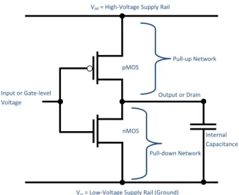
1.3 CMOS NOT logic gate (input-inverter) . . . 15

1.4 Highlighting the focus of this dissertation . . . 24

3.1 Task specifications . . . 41

3.2 Sporadic slack example . . . 45

4.1 Schedule with τ1=h5,10,10i, τ2=h5,16,16i and trn= 1 . . . 52

4.2 “Accumulated delays under EDF scheduling [LRK03]” . . . 53

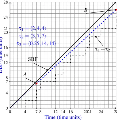
4.3 Schedule with τ1=h2,4,4i,τ2=h3,7,7i and τ3 = h0.25,14,14i . . . 55

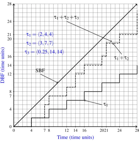
4.4 Demand bound function with tasks τ1=h2,4,4i, τ2=h3,7,7i and τ3=h0.25,14,14i 56 4.5 Procrastination interval for τ2 . . . 59

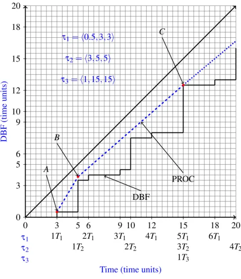
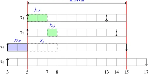
4.6 Static sleep interval with tasks τ1=h0.5,3,3i, τ2=h3,5,5i and τ3=h1,15,15i . 61 4.7 DBF vs SRA . . . 63

4.8 Example to illustrate that ϕ _{≥ χ}min with a task-set composed of τ1=h2,8,8i, τ2=h1,9,9i, τ3=h5,12,12i, τ4=h3,14,14i and χmin= 1 . . . 71

4.9 Variation in Tmax(sleep interval) . . . 82

4.10 Variation in Cb(sleep interval) . . . 82

4.11 Variation in|τ| (sleep interval) . . . 82

4.12 Normalised total energy consumption (ξ1and|τ| = 200) . . . 84

4.13 Gain of ERTH and SRA over LC-EDF for different task-set sizes . . . 84

4.14 Overall-gain of IRTH and LWRTH over ERTH (ξ1) . . . 85

4.15 Sleep threshold effect on total energy of ERTH (|τ| = 50 and ξ1) . . . 85

4.16 Normalised total energy consumption with|τ| = 200 and ξ1 . . . 86

4.17 Overall-gain of IRTH and LWRTH over ERTH (ξ1and Γ0.1) . . . 86

4.18 Variation in Cbfor_{|τ| = 10 (Γ}0.2, ξ1) . . . 88

4.19 Variation in Cbfor|τ| = 50 (Γ0.2, ξ1) . . . 88

4.20 Variation in Γ for|τ| = 50 (ξ1) . . . 89

4.21 Variation in Cb_{in scenario 2 for}_{|τ| = 50 (Γ} 0.2, ξ1) . . . 89

4.22 Temperature profile . . . 95

4.23 Uavailvs ta . . . 95

4.24 Energy vs operating temperature range . . . 96

4.25 Uavailvs operating temperature range . . . 96

4.26 Service curve . . . 98

4.27 Temperature decreases or increase in transition phase . . . 103

4.28 Variation in system utilisation . . . 105

4.29 Variation in execution slack . . . 105 xiii

(18)

4.30 Variation in number of tasks . . . 106

4.31 Variation in sporadic slack . . . 106

4.32 Variation in ˆα . . . 107

4.33 Variation in Pdyn . . . 107

4.34 Number of sleep transitions . . . 108

5.1 Example with two tasks (τ1=h2,10,10,λ1i, τ2=h9,15,15,λ2i) . . . 112

5.2 Low priority workload overlap . . . 120

5.3 Variation in Ω . . . 133 5.4 Variation in|τ| against U . . . 133 5.5 Variation in Γ . . . 134 5.6 Variation in Cb(|τ| = 10) . . . 134 5.7 Variation in Cb(|τ| = 50) . . . 135 5.8 Variation in ξ . . . 135

5.9 Simulation time comparison . . . 136

5.10 Sleep decisions comparison . . . 136

5.11 Efficiency of λEDn i . . . 137 5.12 Variation in τ (|τ| = 5) . . . 137 5.13 Variation in τ (_{|τ| = 50) . . . 138} 5.14 Variation in Γ (|τ| = 50) . . . 138 5.15 Variation in Γ (_{|τ| = 5) . . . 139} 5.16 Variation in Cb(|τ| = 50) . . . 139 5.17 Variation in ξ (|τ| = 50) . . . 139

6.1 Initial schedule when all tasks execute for their WCET . . . 146

6.2 Task τ1generates a slack at time instant 2 . . . 146

6.3 Task τ3starts its execution earlier at time instant 2 . . . 146

6.4 Task τ3generates a slack at time instant 5 . . . 146

6.5 Schedule if τ2executes for its WCET . . . 147

6.6 Schedule when τ2completes early at time t2 . . . 147

6.7 Schedule after a slack donation from πmto πs . . . 147

6.8 Variation in_{|τ| . . . 153}

6.9 Variation in number of cores . . . 153

6.10 Variation in Γ . . . 154

6.11 Variation in Cb(GPM) . . . 154

6.12 Variation in Cb(OverOptimal) . . . 155

7.1 First phase mapping of least loss energy density algorithm . . . 163

7.2 Demand bound function to demonstrate the computation of static sleep interval set in the second phase of optimisation with tasks τ1=h1,4,4i,τ2=h0.75,3,3i and τ3=h0.5,2,2i . . . 166

7.3 (SBET) 4 core types . . . 178

7.4 (SBET) Variation in β . . . 178

7.5 (SBET) Variation in|τ| . . . 179

7.6 (SBET) Asimilar platform . . . 179

7.7 (SBET) 4 core types (WFD) . . . 179

7.8 (SBET) Variation in β (WFD) . . . 179

7.9 (SBET) Variation in|τ| (WFD) . . . 180

(19)

LIST OF FIGURES xv

7.11 (LBET) 4 core types . . . 181

7.12 (LBET) Variation in β . . . 181

7.14 (LBET) Variation in|τ| . . . 181

7.15 (LBET) Variation in_{|τ| . . . 182}

7.16 (LBET) Asimilar platform . . . 182

7.17 (LBET) Decisions . . . 182

7.18 (LBET) Time calculation . . . 182

7.19 (LBET) 4 core types (WFD) . . . 183

7.20 (LBET) Variation in β (WFD) . . . 183

7.21 (LBET) Variation in|τ| (WFD) . . . 183

7.22 (LBET) Asimilar platform (WFD) . . . 183

7.23 Latency hiding instruction scaling . . . 185

7.24 (SBET) 4 core types . . . 186

7.25 (SBET) Variation in β . . . 186

7.26 (SBET) Variation in_{|τ| . . . 187}

7.27 (SBET) Asimilar platform . . . 187

7.28 (LBET) 4 core types . . . 188

7.30 (LBET) Variation in|τ| . . . 189

7.31 (LBET) Asimilar platform . . . 189

A.1 Variation in Tmax(sleep interval) . . . 201

A.2 Variation in Cb(sleep interval) . . . 201

A.3 Variation in_{|τ| (sleep interval) . . . 202}

A.4 Variation in Tmax(REC) . . . 202

A.5 Variation in Cb(REC) . . . 202

A.6 Variation in_{|τ| (REC) . . . 202}

A.7 Normalised total energy consumption (ξ1and|τ| = 200) . . . 204

A.8 Gain of ERTH and SRA over LC-EDF for different task-set sizes . . . 204

A.9 Gain of ERTH and SRA over LC-EDF in idle interval (ξ1) . . . 206

A.10 Gain of ERTH and SRA over LC-EDF in idle interval (ξ2) . . . 206

A.11 Normalised sleep energy consumption (ξ1and|τ| = 200) . . . 207

A.12 Overall-gain of IRTH and LWRTH over ERTH (ξ1) . . . 207

A.13 Normalised average sleep interval (|τ| = 10 and ξ1) . . . 208

A.15 Normalised average sleep interval (_{|τ| = 10 and ξ}2) . . . 209

A.17 Effect of sleep threshold change on total energy consumption of ERTH (_{|τ| = 50} and ξ1) . . . 210

A.18 Effect of sleep threshold change on total energy consumption of LC-EDF (|τ| = 50 and ξ1) . . . 210

A.19 Energy drop on same threshold of the LC-EDF algorithm . . . 210

A.20 Effect of sleep threshold change on total energy consumption of SRA (|τ| = 50 and ξ1) . . . 210

A.21 Effect of sleep threshold Ψ10on ERTH (ξ1) . . . 211

A.22 Effect of sleep threshold Ψ10on LC-EDF (ξ1) . . . 211

A.23 Total energy consumption of ERTH, IRTH and LWRTH at Ψ10with|τ| = 10 and ξ1 . . . 212

(20)

A.24 Effect of two different distributions (ξ1, ξ2) on high sleep threshold (Ψ20) with the

SRA algorithm . . . 212

A.25 Normalised total energy consumption with|τ| = 200 and ξ1 . . . 213

A.26 Overall-gain of ERTH and SRA over LC-EDF (ξ2and Γ0.1) . . . 213

A.27 Overall-gain of ERTH and SRA over LC-EDF (ξ2and Γ0.2) . . . 214

A.28 Overall-gain of IRTH and LWRTH over ERTH (ξ1and Γ0.1) . . . 214

A.29 Variation in Cbfor|τ| = 10 (Γ0.2, ξ1) . . . 216

A.30 Variation in Cbfor_{|τ| = 50 (Γ}0.2, ξ1) . . . 216

A.31 Variation in Γ for_{|τ| = 10 (ξ}1) . . . 218

A.32 Variation in Γ for|τ| = 50 (ξ1) . . . 218

A.33 Variation in ξ for_{|τ| = 10 (Γ}0.2,Cb= 0.5) . . . 219

A.34 Variation in ξ for_{|τ| = 50 (Γ}0.2,Cb= 0.5) . . . 219

A.35 Variation in Cbfor|τ| = 10 (Γ0.2, ξ1) . . . 220

(21)

List of Tables

4.1 Overview of simulator parameters used to evaluate demand bound function based

procrastination . . . 80

4.2 Different sleep states parameters . . . 81

4.3 Overview of simulator parameters used to evaluate alternative race-to-halt algorithms 83 4.4 Overview of simulator parameters used to evaluate thermal-aware energy manage-ment algorithms . . . 104

5.1 Simulator parameters used to evaluate device power management algorithms . . . 132

5.2 Parameters of different devices . . . 133

6.1 Overview of simulator parameters used to evaluate global power management al-gorithm . . . 152

7.1 Tasks allocation through the MM algorithm . . . 164

7.2 Overview of simulator parameters used to evalute non-DVFS heuristics . . . 176

7.3 Heterogeneous multicore platform and its parameters . . . 176

7.4 Overview of simulator parameters used to evaluate the allocation heuristics pro-posed for heterogeneous platform with DVFS capabilities . . . 184

7.5 Frequency specification of the heterogeneous multicore platform . . . 185

A.1 Overview of simulator parameters used to evaluate demand bound function based procrastination . . . 200

A.2 Different sleep states parameters . . . 200 A.3 Overview of simulator parameters used to evaluate alternative race-to-halt algorithms203

(22)

(23)

List of Algorithms

1 Slack Management . . . 46

2 Enhanced Race-To-Halt Algorithm (ERTH) . . . 68

3 Common Routines for ERTH, IRTH and LWRTH . . . 69

4 Improved Race-To-Halt Algorithm (IRTH) . . . 74

5 Light-Weight Race-To-Halt Algorithm (LWRTH) . . . 76

6 Static Slack Container Algorithm (SSC) . . . 114 7 Device Budget Reclamation Algorithm . . . 122 8 Offline Algorithm for Multiple Sleep State Devices (SSCo) . . . 127 9 Static Slack Container Algorithm for Multiple Sleep State Devices (SSCm) . . . . 129 10 Aggressive Static Slack Container Algorithm for Multiple Sleep State Devices

(SSCa) . . . 130

11 Global Power Management Algorithm (GPM) . . . 149

12 First Phase: Least Loss Energy Density (LLED) . . . 162

13 Alternative First Phase: Maximum Minimum (MM) . . . 163

14 Second Phase of Task Mapping (SP) . . . 165 15 First Phase of Allocation . . . 170 16 Second Phase of Optimisation (SP) . . . 173

(24)

(25)

List of Acronyms

ABS Anti-lock breaking system

ACU Air-bag control unit

API Application programming interface

ASIC Application specific integrated circuit

BCET Best-case execution time

BE Best effort

BET Break-even-time

ccEDF Cycle-conservative earliest deadline first

CMOS Complementary metal-oxide-semiconductor

COLORS Composite low-power scheduling framework

Cons Consumption

CPU Central processing unit

DBF Demand bound function

DBFP Demand bound function based procrastination

DD Density difference

DFA Dynamic frequency allocation

DFA-LP Dynamic frequency allocation with reduced pessimism

DFR-RMS Device forbidden regions algorithm for rate monotonic schedulers

DIBL Drain-induced barrier lowering

DJP Dynamic job priority

DM Deadline monotonic

DM-PM Deadline monotonic with priority migration

Don Donation

DPM Dynamic power management

DTM Dynamic thermal management

DVFS Dynamic voltage and frequency scaling

DVS Dynamic voltage scaling

ED Energy density

EDF Earliest deadline first

EDS Energy-optimal device scheduler

EEC Expected energy consumption

EEDS Energy efficient device scheduling

ERTH Enhanced race-to-halt

ESSR Execution slack service register

FF First-fit

FIFO First-in-first-out

FJP Fixed job priority

FPGA Field programmable gate array

(26)

FRT Firm real time

FTP Fixed task priority

GEDF Global earliest deadline first

GIDL Gate-induced drain leakage

Global-EDF Global earliest deadline first

GPM Global power management

GPS Global positioning system

HDMI High-definition multimedia interface

HPW High priority workload

HRT Hard real-time

HyWGA Hybrid worst-fit genetic algorithm

I/O Input/Output

IC Integrated circuit

ILP Integer linear programming

IPW Intermediate priority workload

IRTH Improved race-to-halt

ISR Interrupt service routine

ITRS International technology roadmap for semiconductors

LBET Low break-even-time

LC-DP Leakage control dynamic priority

LC-EDF Leakage control earliest deadline first

LCM Least common multiple

LEDES Low energy device scheduler

LLED Least Lost energy density

LLED-SP Least lost energy density and second phase

LLF Least laxity first

LLREF Largest local remaining execution first

LP Linear programming

LPW Low priority workload

LQS Low-power quasi-dynamic scheduling

LRE-TL Local remaining execution TL-Plane

LWRTH Light-weight race-to-halt

MDO Maximum device overlap

MM Maximum minimum

MM-SP Maximum minimum with second phase

MOSFET Metal-oxide-semiconductor field-effect transistors

MT Matrix

MUSCLES Multi-state constrained low-energy scheduler

nMOS n-type metal-oxide-semiconductor field-effect transistors

NS Without sleep states

PARTPN Power-aware real-time petri-nets

PDMS_HPTS Partitioned deadline monotonic scheduling with highest priority task split

PF Proportionate progress

PLL Phase lock loop

pMOS p-type metal-oxide-semiconductor field-effect transistors

PROC Procrastination algorithm based on Jejurikar et al. [JPG04] method

PUB Period upper bound

(27)

List of Acronyms xxiii

RBED Rate-based earliest deadline first

REC Reducible energy consumption

RM Rate monotonic

ROM Read only memory

RT Real-time

RTH Race-to-halt

RTOS Real-time operating system

SBET Small break-even-time

SBF Supply bound function

SFA Static frequency allocation

SMP Symmetric multicore platform

SMS Short message service

SP Second phase

SPARTS Simulator for power aware and real-time systems

SRA Slack reclamation algorithm

SRT Soft real-time

SSC Static slack container

SSSR Static slack service register

staticEDF Static earliest deadline first

TCDPM Thermally constrained dynamic power management

TE Total energy

TTL Transistor-transistor logic

USB Universal serial bus

WCET Worst-case execution time

(28)

(29)

List of Symbols

Hardware Platform Symbols

Hardware Platform π

No of processor types M

Processor index m

Processor type m πm

Task-set allocated to a processor type m τm

Active power of a processor P_Am

Idle power of a processor P_Im

Vector of sleep states §~m

Sleep index n

Number of sleep states N

Sleep state of a processor §mn

Power of a sleep state P_nm

Transition delay of going into a sleep state tsm_n

Transition delay of going out of a sleep state twm_n

Complete transition delay tswm_n

Transition delay trm_n

Power dissipated in transition phase Ptrm_n

Energy overhead of a sleep state Esm_n

Break-even-time of a sleep state bet_nm

Average sleep energy E¯§mn

Sleep threshold Ψ

Vector of frequencies ~fm

Frequency index v

Number of frequencies Vm

Frequency of a processor f_vm

Power dissipation at a frequency Pm_fm

v

Critical speed f_critm

Dynamic power dissipation Pdyn

Leakage power dissipation Plkg

Short circuit power dissipation Pshort

Total power dissipation Ptotal

Energy E

Expected energy consumption EEC_vm

Frequency Combination Λi

Set of frequency combinations Λ

Energy consumption per unit time in the idle mode S fe

Total Energy TE

(30)

Speed up factor κm

Helper variable ζ

Average capacity of the heterogeneous platform Uavg

Effective utilisation of the hardware platform Ue f f

System Model Symbols

Time t Task-set τ Task-set size ` Total utilisation U Task index i Task τi

Worst-case execution time Ci

Average-case execution time C¯i

Relative deadline Di

Minimum inter-arrival time Ti

Average minimum inter-arrival time T¯i

Actual allocated budget Ai

Individual Task utilisation Ui

Job index k

Job ji,k

Absolute deadline di,k

Release time r_i,k

Current budget ai,k

Actual execution time ci,k

Hyper-period H

Task-set distribution ξ

Sporadic delay limit Γ

Best-case execution time limit Cb

Sporadic delay limit of a task Γi

Best-case execution time limit of a task C_ib

Vector of execution profiles of τion different core types

⇒

Ci

Vector of WCET of a task on a specific core type at different frequencies C→_im

WCET at specific frequency C_i,vm

WCET at maximum frequency C_im

Average execution time at maximum frequency C¯_im

Vector of average energy consumption profiles of τion different core types

⇒

¯ Ei

Vector of average energy consumption of a task on a specific core type at dif-ferent frequencies

¯ E_im

Average energy consumption at specific frequency E¯_i,vm

Average energy consumption at maximum frequency E¯_im

Utilisation of a core type m Um

Utilisation of a core type m at frequency v Um,v

Minimum idle interval or Static sleep interval χminm

Set of static sleep interval χm

Shortest gap in the schedule ρ

(31)

List of Symbols xxvii

Minimum procrastination interval computed through PROC Zmin

Timer ϖ

Individual utilisation of task on a core type m at frequency v U_i,vm

Characteristics factor to model task’s behaviour β

Density difference DDm_i

Energy density EDm_i

Group of tasks to enable specific sleep state Gm_n

Local cost of migration of a task LC_τm

i

Device Model Symbols

Number of devices W

Set of Devices λ

Device λi

Active power dissipation of a device Pλi

A

Vector of device sleep states §~λi

Sleep state of a device §λi

n

Power dissipation of a device in a sleep state Pλi

n

Transition overhead of going into a device’s sleep state tsλi

n

Wake-up transition overhead of a device’s sleep state twλi

n

Complete transition overhead of a device’s sleep state tswλi

n

Transition overhead of a device’s sleep state trλi

n

Power dissipated in the transition phase of a device’s sleep state Ptrλi

n

Energy consumption in the transition phase of a device’s sleep state Esλi

n

Break-even-time of a device’s sleep state betλi

n

Static slack container SSC

Offline algorithm for multiple sleep states devices SSCo

Static slack container algorithm with multiples sleep states per devices SSCm Aggressive static slack container algorithm with multiples sleep states per

de-vices

SSCa

Set of all sleep states of devices in the system φ

Intra-task device compatible Φ

Device budget Db

Pending high priority workload Ξt_i

Device transition start time λ_istart

Device ready time λ_iready

Device in transition phase λt

Energy density function of a device λ_iEDn

Device percentage usage time Ω

Next utilisation time of a device λiNU T

Slack Sources Symbols

Execution slack Se

Size of execution slack Ssz_e

Deadline of execution slack Sdl

e

Usable execution slack Su_e

Not usable execution slack Snu_e

Usable idle slack Su_i

(32)

Set of next earliest release time γ

Earliest release time of a task γi

ithelement of sorted γ γ(i)

Thermal Aware Design Symbols

Temperature T m

Available utilisation Uavail

Requested utilisation Ureq

Time of cooling phase tc

Time of active phase ta

Start time of active phase ˆt

Temperature at time instant ˆt+ t Tact(ˆt,t)

Start time of cooling phase ˇt

Temperature at the end of the interval(ˇt, ˇt+ t] Tdor(ˇt,t)

Current I

Average current I¯

Voltage V

(33)

Chapter 1

Introduction

1.1 Embedded Systems

The technology evolution has made embedded systems an integral part of our life. These systems perform a set of dedicated functions and interact with their environment. In fact most of the embed-ded systems are hidden from our eyes and thus make us forget their existence. These sophisticated systems are rapidly replacing complex jobs previously preformed by human evolving our society to the era of automation. These systems not only reduce the risk of failure as humans are prone to errors but also provide increased precision and high efficiency previously not possible with human interaction. Up to some extent, the credit goes to these systems that have raised our quality of life in this modern era of computing. Nowadays, embedded systems are deployed in various aspect of our life. Typical domains in which such systems are deployed includes consumer electronics, medical equipment, avionics, automotive industry, banking, and defence industry [Noe05, Nel11]. The list is not limited to the aforementioned domains. Despite their existence in a variety of dif-ferent domains, the basic principles of their design tend to resemble. Before going into the details of embedded system design, trends, challenges and constraints, lets visit a definition of this term. The term “embedded system” is not rigorously defined in the literature. Experts in the field have come up with different meaning of this term corresponding to different properties, features and constraints of embedded systems. Some of the definitions from various experts in the domain are summarised by Raj Kamal [Kam03]. In the context of this thesis, an embedded system is defined as follows.

Definition 1. An embedded system is a microprocessor-based system composed of hardware, soft-ware and/or mechanical components to perform a dedicated function or a range of functions.

These dedicated functions vary from a simple task of toasting a slice of bread to an air traffic control system that involves numerous workstations, networks and radar sites. Nevertheless, an embedded system is still considered different from general purpose computer system designed to satisfy a variety of end-user requirements. A general purpose computer system provides a flexibility to craft the system according to the needs of a user and designed to run a variety of applications. The desired functionality of an embedded system is usually known at design time.

(34)

The information on dedicated function or a range of functions that an embedded system is desired to perform allows to design these systems with optimised software and hardware capabilities.

In general, an embedded system is designed to provide extra reliability over its counterpart general purpose computing system such as a personal computer. Some embedded systems are mission critical such as aircraft flight control and satellites, and any malfunction in such systems can risk human life, equipment damage, property loss and mission failure. Embedded systems deployed in avionics, automotive industry, industrial controllers and military equipments have to deal with vibration, shock, extreme heat, cold and radiations. Contrary to personal computers, the luxury of a software update is also sometimes trickier as these systems are embedded inside a big system and/or deployed in remote areas such as undersea applications or space voyagers. These system must have a mechanism to solve its issues remotely. On top of this, any faults that leads to a failure of the system can also destroy the reputation of a manufacturer. Therefore, such systems are exhaustively tested in their design phase to ensure their functional correctness. Such reliability in personal computers is hard to maintain due to the dynamic nature of applications designed by various third party companies with different tools and made compatible for a variety of hardware platforms available in the market.

Another strict requirement over the dimensions (weight and size) of an embedded system is usually dictated by aesthetics or a limitation to fit in interstices among mechanical parts. Users demand to increase the endurance also prompts a system designer to optimise the dimensions of embedded systems. The extra fuel cost in transportation system and space ventures is another factor that imposes size and weight constraint on embedded systems. Similar to other technology markets, embedded systems in the consumer electronics domain are sold in a very competitive market. The cost sensitivity is usually attached with the performance, precision and the quantity of items produced. For example, a management is less sensitive to a cost issue of a high end embedded system produced in a small quantity when compared to a system produced in an order of millions. Time-to-market is another important constraint that system designers has to cope with. The designers need to deliver systems on time to gain a maximum advantage out of their product and have to adopt very quickly according to new technology trends. One of the recent example is Nokia in the market of mobile systems. Nokia [Cor] has a dominating market share in the mobile phone industry in the last decade. Samsung [Gro] brought its smart-phones very quickly in the market and acquired a large share in the mobile industry.

The primary requirement of an embedded system is to correctly perform a desired functional-ity. There is a class of embedded systems that has an additional constraint of temporal requirement to be met on top of the functional correctness for the overall system to be considered correct. This class of embedded systems is named as real-time (RT) systems in the literature. Consider an ex-ample of an anti-lock breaking system (ABS) in cars. The RT or temporal constraint in this system requires to release breaks for a very short period of time before reaching the skidding point that may cause the car to get out of a driver’s control. The timing is an important property of the sys-tem as a minor delay can cause a syssys-tem failure. Stephan J. Young [You82] formally defined a RT system as follows.

(35)

1.1 Embedded Systems 3

Definition 2. “Any information processing activity or system which has to respond to externally generated input stimuli within a finite and specified period.” — Stephan J. Young[You82]

Similarly, Oxford dictionary of computing [Wri] gives the following comprehensive definition of a RT system.

Definition 3. “Any system in which the time at which output is produced is significant. This is usually because the input corresponds to some movement in the physical world, and the output has to relate to that some movement. The lag from input time to output time must be sufficiently small for acceptable timeliness.” — Oxford Dictionary of Computing [Wri]

These definitions cover a wide range of RT systems but fortunately, all these different RT systems can be classified into two main categories depending on the nature of timing require-ment [BW09]. These two different categories of RT systems are given as follows.

• Hard Real-Time Systems: Hard real-time systems (HRT) are the class of embedded sys-tems in which a desired operation violating the temporal constraint, i.e., completing after the predefined time interval, may cause catastrophic or irreversible consequences. In other words, it is imperative to meet the timing requirements regardless of a system’s state. The constraint on the timing is commonly known as a deadline. These catastrophic or irre-versible consequences may lead to a damage to the physical surrounding or threaten human life. The results obtained after a given time interval (or deadline) are considered useless in HRT systems. A simple example is an operation of an air-bag in our modern cars. The air-bag control unit (ACU) must inflate the fabric bag within 60-80 milliseconds after the first moment of a car’s contact with the opposing object in case of an accident. ACU failing to meet this specification may even increase the risk of injury to the persons inside the car. Another example of a HRT system is an automatically controlled train. The train cannot stop immediately. In order to stop the train at some desired point say x, it must activate the break command a certain distance away from x. The controller of the train considers the safe deceleration rate and the speed of the train to compute the distance before x to apply breaks. Any delay in computation and/or activating the break command my cause disastrous consequences. Similarly, other examples of HRT systems are artificial heart pacemaker that regulate the beating of a heart patient, industrial process controllers, ABS, engine control system etc.

This thesis focuses on HRT systems.

• Soft Real-Time Systems: Opposed to HRT systems, soft real-time systems (SRT) can tol-erate occasional temporal violations, but the significance of the results degrades with the passage of time after their deadline. In literature, the usefulness of the results is sometimes referred to as tardiness. A desired function completing before or at its deadline has tardi-ness equal to zero. An operation failing to meet its deadline has a tarditardi-ness equal to the

(36)

difference between the completion time of an operation and its deadline. It is desirable to meet all deadlines and minimise tardiness if not all deadlines can be met. However, it does not cause dire consequences due to any misbehaviour in the timing constraint. For exam-ple, a degradation in the quality of electronics games is annoying but not life threatening. Similarly, a delay in the online transaction system will not cause the whole system to crash but can be extremely expensive. The degradation in the usefulness of the results can be demonstrated with the stock price quotation system [Liu00]. It is desirable to update the price of each stock as soon as its price changes. The delay in the price change reduces the usefulness of the results with time. Additionally, SRT systems in which the results are no more valuable after the deadline miss but such a situation does not have any catastrophic consequences (as in HRT systems deadline miss) are said to have firm deadlines. A delay in the video conferencing application causes a drop of frames after their deadline miss and people experience some glitches. Similarly, the quality of the voice in phone calls is another example. The validation of a SRT system is not as rigorous as it is performed in a HRT system and it allows system designers to focus on other performance metrics as well.

Many embedded devices are nomadic and have limited energy supply. Such energy constraints are induced by e.g., battery powered mobile devices or those with limited or intermittent power supply such as solar cells. Apart from limited power supply, some embedded systems also have thermal issues. Satellites are the prominent example of such systems. Reasons to reduce the energy consumption of an embedded system include the following.

1. The high requirement of the energy can lead to an increase in the size of an embedded system which is not desirable in many cases such as consumer electronics, avionics, automotive industry and military equipments.

2. A longer lasting battery is a market differentiator. Consumer always opts for a system that offers extra battery life with same functionality to avoid the hassle of recharging and increase its mobility. A system optimised for energy consumption is especially useful in scenarios where frequent battery replacements are very costly such as sensor networks deployed in remote areas.

3. High energy requirement causes thermal issues which in turn increase the packaging cost of an embedded system and/or demands efficient cooling systems. Thermal issues also affect the speed, power and reliability of the semiconductor chips [WA11].

4. Energy savings have positive impact on the environment. Batteries used in embedded sys-tems are usually made from harmful chemical such as cadmium, lead and mercury [BET04]. These chemical can effect the living beings as batteries are usually dumped in fields. The lack of recycling and disposal sites is currently a major issue.

(37)

1.2 Basic Components of Real-Time Systems 5

1.2 Basic Components of Real-Time Systems

A RT system may be viewed as three main components called applications, real-time operating system (RTOS) and hardware platform. The interaction between these components is demon-strated in Figure 1.1. Applications correspond to the dedicated functionality that a RT system is desired to perform on a given hardware platform. A real-time operating system sits in between a hardware platform and a given applications to provide hardware abstraction, perform scheduling and facilitate communication. It provides application programming interfaces (API) to allow the interaction of the application with the given hardware platform and the given application can ac-cess the different components of the hardware platform through available API’s. Please note that a small scale RT system may not have an RTOS. The source code of the application is compiled and stored in a read only memory (ROM) to access the hardware platform. For example, a simple RT system that monitors the temperature of a room does not require a complex RTOS. Nevertheless, an RTOS is assumed to be a part of a RT system in the context of this dissertation. The hardware platform provides the physical layer that executes the given application. These basic components involved in the design of RT systems are discussed here providing us a base to explore the main topic of this dissertation, i.e., energy and thermal management.

Hardware Platform Real-Time Operating System

Applications

Figure 1.1: Different components of a RT system

1.2.1 Applications

Real-Time applications are usually represented by an abstract workload model that specifies the relevant characteristics of the workload generated by such applications when analysing a system. The functionality of a RT application can be modelled as a finite collections of simple, highly repetitive or abstract entities called real-time tasks [BG03]. These tasks are recurrent in nature. Each instance of a task is a basic unit of work that executes on the physical hardware platform and is called a RT job or in short a job [Liu00]. All jobs related to a particular task are semantically related. From now onwards, the functionality of a RT application is represented as a set of tasks called task-set. A frequency with which a task releases its jobs can be categorised into three types [IF00].

(38)

• Periodic Tasks: A task that releases its jobs periodically after a fixed time interval is defined as a periodic task. The fixed duration between the two consecutive jobs releases is called a period of a task.

• Sporadic Tasks: A task that releases its jobs at some arbitrary time instant but the two consecutive jobs of a task are always separated by at least a predefined time interval called minimum inter-arrival time.

• Aperiodic Tasks: Jobs of an aperiodic task is not constrained by a minimum inter-arrival time or a period, it can release jobs at any instant.

Within this work the focus is on sporadic tasks.

RT tasks are always constrained with a timing requirement. A task should complete its ex-ecution within a predefined time interval called the relative deadline of a task. A task failing to generate desired results within its relative deadline can jeopardise the whole system, environment or user’s safety. A relative deadline of a task depends on the nature of an application. For exam-ple, the air-bag application installed in a car has a relative deadline of 60-80 milliseconds, while a room temperature monitoring application can have a relative deadline of a few seconds. A relative deadline of a periodic or a sporadic task can be categorised into three main classes.

• Implicit Deadline Task: An implicit deadline task has a relative deadline equal to its period or minimum inter-arrival time.

• Constrained Deadline Task: A constrained deadline task may have a relative deadline less than or equal to its period or minimum inter-arrival time.

• Arbitrary Deadline Task: As the name implies, an arbitrary deadline task has no relation with the period or minimum inter-arrival time of a task. It means that multiple jobs of the same task may be released with a difference of minimum inter-arrival time and coexist in the ready queue.

This work focuses on constrained deadline tasks.

The execution time of a task is another parameter that must be specified to characterise its temporal behaviour. Different jobs of a task exhibit variation in their execution time depending on the hardware characteristics, structure of the software, input data and different behaviour of the environment with which such job is interacting. In order to guarantee the temporal correctness, the upper bound on the execution time of a task is specified called worst-case execution time (WCET). The WCET of a task is the safe upper bound beyond or equal to the longest execution of any job released by such task. However, there is an assumption that execution times of the jobs are measured without any interruption. Any miscalculation in this parameter may cause a system failure. The term WCET is introduced formally in Definition 4. There are numerous methods and

(39)

techniques to compute the WCET of a task and the interested reader is directed to the following surveys of such techniques for further reference [PB00, WEE+08]. RT system designers consider the WCET of tasks while designing a system to guarantee the timing properties, however, different jobs of a task may execute for less than their WCET leaving behind unused computing resource. This bound must be pessimistic to be safe.

Definition 4 (WCET). Assume processor is in any legal state at the beginning of an execution of a task then the worst-case execution time of a task on a given hardware platform is the maximum length of its execution time, under worst-case input conditions without considering interference from other tasks.

The nature of the application sometimes demands precedence constraints and data dependen-cies among tasks. For example, the inflate task in the air-bag system is dependent on the data from the sensor that provides information about the intensity of an impact in case of an accident. Simi-larly, the authentication task is performed before the access tasks in most of the banking systems. The type of tasks that needs to perform their execution in some order are said to have a precedence constraint. The tasks that can perform their execution without any order are called independent tasks. Such a task does not depended on the outcome of any other task or tasks to initiate their execution. For example, toast a slice of bread with the given temperature. Similarly, displaying the sensor reading of different parameters in the system on the monitor. The collection and display of data from a specific sensor can be performed independent of each other. Please note that the term task and job are used interchangeably in this dissertation. An execution of a task implicitly corresponds to the execution of its job.

This work focuses on independent tasks.

1.2.2 Real-Time Operating System

A real-time operating system is tailored for RT applications and designed to provide predictability and reliability in the system. The term predictability means the ability of the system to guar-antee the timing properties at design time. The term reliability means “the ability of a system or component to perform its required functions under stated conditions for a specified period of time”[Dec98]. One of the main objectives of an RTOS is to provide an interface between RT tasks and resources available on the hardware platform. Furthermore, it provides an abstraction of the underlying hardware platform, and facilitates scheduling and communication. As the resources are usually limited in such platforms, therefore, it also coordinates and arbitrates their allocation among different tasks. Examples of an RTOS include VxWorks, RTEMS and PikeOS. The Mars reconnaissance orbiter and curiosity rover sent to the Mars used VxWorks as the operating system. RTEMS is commonly used in space applications, while PikeOS targets safety and security critical embedded systems. Similar to any other general purpose operating system, API’s of an RTOS relieves the programmer of a RT application to worry about the hardware details. These API’s

(40)

are optimised for different types of hardware platforms. Typically an RTOS performs many activ-ities such as task management (scheduling), interrupt handling, memory management, inter-task communication and resource sharing. Nevertheless, the discussion in this section is limited to task management or scheduling.

A scheduler is a mechanism by which the RTOS allocates resources (such as processor) to tasks to perform their execution. It decides the time instant and the duration of execution for each task. Scheduling in RT systems has been widely studied in the literature. There exist nu-merous scheduling techniques for a vast variety of systems and task-models. Initially, scheduling techniques for a single processor were studied and later extended to the multiple processors case. Scheduling algorithms can be classified based on many factors. For example, scheduling algo-rithms can be divided into online and offline algoalgo-rithms. In an online algorithm, the scheduling decisions are made based on the current state of a system, while in an offline scheduling algorithm, a precomputed schedule is determined offline. However, this section adopts the classification pro-posed by Jane Liu [Liu00]. She divides scheduling algorithms into following three main classes. 1) Clock Driven Scheduling: Clock driven scheduling approaches are also commonly known

as time driven scheduling algorithms. In this category of algorithms, the scheduling decisions — which job executes at what time instant — are made at predefined time instances. Such decisions are made offline and stored in a memory to access online. The task parameters are usually fixed in this type of scheduling algorithms and a designer has complete knowledge available a-priori to derive a static schedule. Usually, the complete static schedule is divided into frames. The scheduling decisions are made at the boundaries of each frame. The size of a frame is selected consciously such that it minimises the scheduling overhead. The static schedule is repeated in a cyclic manner. A clock driven scheduling is a very simple approach. Its online complexity is very low as the schedule is precomputed. In this approach, scheduling tables can be easily replaced in different operating modes. The context switching overhead can be reduced by optimising the frame size. Many traditional RT systems are scheduled through this technique such as a traditional flight control systems or health care systems. These schedules are easy to validate, test and certify. The disadvantage of such a system includes its fixed nature. Any alteration in the task-set needs a redesign of a static schedule. Hence, it is suited for a fixed small embedded controller that rarely requires any changes.

2) Round Robin Scheduling: Round robin scheduling algorithms are suitable for time shared applications. Jobs in this strategy are placed in a first-in-first-out (FIFO) queue. Each job on the head of FIFO queue gets a same share of time. A job not completing in this share is pre-empted and added at the end of the FIFO queue. The time sharing slowly progresses the execution of all jobs. This algorithm is sometimes called a processor-sharing algorithm. One of the variation of such algorithm is a weighted round robin scheduling algorithm. Each job is allocated a specific share in FIFO order. The complete round of such algorithm is a summation of such weights allocated to different jobs in the FIFO queue. Weighed round robin is commonly used for RT traffic in high-speed switched networks [Liu00].

(41)

3) Priority Driven Scheduling: In a priority driven scheduling algorithm, tasks or jobs are allo-cated a priority and scheduled accordingly. The priorities can be alloallo-cated based on different criterion such as earliest deadline first, least laxity first, arrival rate of a task, shortest execution time first, shortest deadline first etc. The priorities of jobs or tasks can be allocated statically at design time or dynamically at run time. Most of the research effort is dedicated in this category of scheduling algorithm in a RT context. The pioneer work of Liu and Layland [LL73] on dy-namic priority scheduling algorithm called earliest deadline first (EDF) scheduling algorithm and fixed priority scheduling algorithm, and the work of Mok [Mok83a] on least laxity first (LLF) are some examples of this class of scheduling algorithm. The priority driven scheduling approach can be further divided into three main categories.

(a) Fixed Task Priority (FTP): In a fixed task priority scheduling algorithm, priorities are assigned to tasks. All the instances of a task (i.e., all its jobs) inherit the same priority. The priority of a job remains static through out the execution time. There are various prior-ity assignment algorithms such as rate-monotonic (RM) [LL73] and deadline-monotonic (DM) [LW82]. Usually, the priority is assigned based on certain property of a task. In case of the DM priority assignment algorithm, a task with the shortest deadline is as-signed the highest priority. Similarly, in the RM priority assignment algorithm, a task with smallest period is assigned the highest priority.

(b) Fixed Job Priority (FJP): In this category of priority scheduling algorithm, priorities are assigned to jobs rather than their tasks. It means that different jobs of the same task may execute on a processor with different priorities. The priority of the certain job remains the same between its release time and deadline. There are many scheduling algorithms that falls in this category such as optimal EDF algorithm [LL73], earliest deadline Deferrable Portion (EDDP) [KY08] and EDF with C= D [BDWZ12]. The priority of a job in this class of algorithms is usually assigned based on the fixed property of a job. For example, in case of EDF, the absolute deadline of a job is the fixed property that does not change throughout its active time.

(c) Dynamic Job Priority (DJP): This is the most general form of a priority driven schedul-ing scheme. The priority of a job may change at any instant durschedul-ing its execution. One of the examples in this category is the LLF scheduling algorithm [Mok83a]. The priority of a job in LLF depends on the job’s laxity (its deadline minus its remaining execution time). A job with the minimum laxity is allocated the highest priority and vice versa. The priority of a job varies with its execution on a processor. Such systems are difficult to design and may suffer from high number of pre-emptions. Other examples of such al-gorithms include proportionate progress (PF) [BCPV93], local remaining execution TL-Plane (LRE-TL) [Fun10] and largest local remaining execution first (LLREF) [CRJ06].

This work focuses on a rate-based scheduling approach with EDF and in particular considers fixed job priority schedulers at its core.