Mortality and Longevity Projections for the Oldest-Old in Portugal

(1)

M

ORTALITY AND

L

ONGEVITY

P

ROJECTIONS FOR THE

O

LDEST

-O

LD IN

P

ORTUGAL

Edviges Coelho

Statistics Portugal – Department of Demographic and Social Statistics (edviges.coelho@ine.pt)

Maria Graça Magalhães

Statistics Portugal – Department of Demographic and Social Statistics (mgraca.magalhaes@ine.pt)

Jorge Miguel Bravo

University of Évora - Department of Economics and CEFAGE-UE / CIEF (jbravo@uevora.pt)

* The analyses, opinions and findings contained in this paper represent the views of the authors and are not necessarily those of Statistics Portugal.

ABSTRACT

The mortality decline observed in developed countries over the last decades significantly increased the number of those surviving up to older ages. Mortality improvements are naturally viewed as a positive change for individuals and as a substantial social achievement for societies, but create new challenges in a number of different areas, ranging from the planning of all components of social security systems to labour markets. Understanding mortality and survival patterns at older ages is crucial. In this paper, we compare the results provided by a number of different methods designed to project mortality for the oldest-old in the Portuguese population. We identify the merits and limitations of each method and the consequences of their use in constructing complete life tables.

Keywords: mortality, life tables, projection models, life expectancy

1. Introduction

Life expectancy at birth more than doubled in Portugal during the XX century. Based on all available demographic databases, historical trends show that both average and the maximum lifetime have increased gradually during the 20th century, with human life span showing no signs of approaching a fixed limit imposed by biology.

As in other developed countries, the mortality decline has been dominated by two major trends: a huge reduction in mortality due to infectious diseases affecting mainly young ages, more evident during the first half of the century, and a decrease in mortality at older ages, more pronounced during the second half. As a consequence, the number of those surviving up to older ages (e.g., 80 years and above) has increased significantly representing, in 2006, 4.9% (2.9%) of the Portuguese female (male) population.1 Additionally, the number of deaths of the oldest-old accounts for an increasing proportion of all deaths, with reductions of mortality beyond these ages having a growing contribution to future gains in life expectancy.

1_{According to the United Nations (2001), it is estimated that in 2001 the population of the oldest-old (i.e., those 80 years}

and older) represents 1.2% of the 6.1 billion inhabitants of the world, being the fastest growing segment of the population.

(2)

Mortality improvements are naturally viewed as a positive change for individuals and as a substantial social achievement for developed countries. Nonetheless, this change poses a serious challenge in a number of different areas, ranging from the planning of all components of social security systems (e.g., public and private retirement systems, health care systems) to labour markets and economic models. In the insurance market, mortality improvements have an obvious impact on the pricing and reserving for any kind of long-term living benefits, particularly on annuities.

In view of these trends, it is important not only to have a clear understanding of mortality and survival patterns at older ages, namely about their age structure, but also about the population dynamics to which they are subject. In Portugal, as in most countries, population estimates and projections produced by the Statistics Portugal (INE – Instituto Nacional de Estatística) do not provide an age breakdown for the group aged 85 years and older. Although rough data on population estimates at these ages is available, except for censuses years they are considered unreliable, being biased by poor age reporting regarding both those alive and who die. Because of this, crude estimates of mortality rates by single year for people aged 85 and over may lack the required quality demanded for the construction of complete life span lifetables. To solve this problem we have to resort to projection models that describe appropriately the main mortality trends observed at these ages.

In recent years, the improvement of statistical data shed light on an apparently unexpected behaviour of mortality at advanced ages. Effectively, empirical evidence (e.g., Horiuchi and Wilmoth, 1998; Olshansky and Carnes, 1997; Wilmoth, 1995; Bongaarts, 2004; Gallop and Macdonald, 2005) shows that the rate of mortality increase at very old ages is neither increasing nor constant, but rather tends to decelerate from a certain age. In particular, the curve of mortality rates, in logarithmic scale, presents a concave shape for high ages, leading to a sort of "plateau". This mortality pattern diverges from that stipulated, e.g., by the classical Gompertz law, for which mortality increases exponentially with age. The simple Gompertz law has proven to be a remarkably good model in different populations and in different epochs, and many subsequent mortality laws are indeed modifications of it, made to account for known deviations, for example, at very old ages. However, these latest developments reveal that the model can no longer provide a good description of data.

Various methodologies have been proposed for estimating mortality rates at oldest ages. Some generate population numbers from death registrations, which for the purpose of estimating the number of very old people are considered to be more reliable than population estimates derived from censuses. The most popular methods included in this category are the method of extinct generations and the survivor ratio method.

Other methodologies include fitting mortality curves over a certain age range, for which crude mortality rates may be calculated directly from data, followed by extrapolation. The incapacity of classic mortality laws to represent the modern behaviour of mortality at advanced ages, with a clear departure from trajectories generated by the classical Gompertz model has, in recent

(3)

years, attracted the attention of researchers in both the demographic and actuarial area towards the development of alternative formulations that better capture this phenomenon. The number of alternative models proposed in the literature is vast and growing (see, e.g., Boleslawski and Tabeau (2001), Buettner (2002) and Pitacco (2004)). Among these, we investigate in this paper two versions of the logistic model, namely those suggested by Perks (1932) and Kannistö (1992), the method of Coale and Kisker (1990) and the recently proposed method of Denuit and Goderniaux (2005).2

The objective of this study is two-fold: (i) to compare the merits and disadvantages of different methods used to extrapolate mortality rates at older ages (ii) to measure the impact of these models in terms life expectancy calculations, briefly discussing the consequences of their use in mortality and longevity projections. The database used in this study was provided by the NSI and comprises the observed number of deaths given by age and year of birth, and the observed population size at December 31 of each year.

The paper is organized as follows. Section 2 presents a brief characterization of the evolution of mortality patterns in Portugal. Section 3 gives an overview of the available population and death data and discusses some of the problems encountered in estimating mortality rates at old ages. Section 4 describes a number of approaches in estimating mortality rates at advanced ages. Section 5 presents the results and discusses the ability of each model in describing the mortality at these ages. Finally, Section 6 provides a short conclusion.

2. Mortality trends in Portugal

The XX century saw dramatic reductions in mortality rates at all ages in Portugal. Two major trends dominated the mortality decline during the last century: a huge decrease in infant mortality, more evident during the first half of the century, and a decrease in mortality at older ages, more pronounced during the second half. This clear change in mortality patterns led to an increase in the number of those surviving up to ages 80-85 years, with reductions of mortality beyond these ages having a growing contribution to future gains in life expectancy.

In 1950, around half of all deaths occurred under age 50. In the same year, infant mortality accounted for 19% of all deaths, whereas deaths at age 80 and over comprised only 13.8%. In 2006, there were 101 948 deaths of resident individuals in Portugal, the majority of which (81%) occurred at age 65 and over, whereas 47% of all deaths were registered at ages 80 and above. Deaths at ages under one year (infant mortality) represented only 0.3%.

In Figure 1 we represent the distribution of the number of deaths at different ages (i.e., of the graph of the function

x

a

d

_x

/

l

₀_{) for a number of selected moments from 1950 to 2006. In both}

sexes, we can observe an increasing concentration of deaths around the mode (age of

2_{Other formulations such as the Heligman-Pollard (1980) model, the logit model (Brass, 1971) and the Lindbergson}

(4)

maximum mortality) of the distribution, as well as a shift in the mode towards older ages. As a result, Figure 2 shows a progressive rectangularization and expansion of the survival curve, most noticeably for the female population.

Figure 1 – Curves of deaths (

x

a

d

_x

/

l

₀_{), Portugal}

M ale 0,00 0,01 0,02 0,03 0,04 0,05 0,06 dx/l0 M 1950 dx/l0 M 1980 dx/l0 M 1990 dx/l0 M 2000 dx/l0 M 2006 Female 0,00 0,01 0,02 0,03 0,04 0,05 0,06 dx/l0 F 1950 dx/l0 F 1980 dx/l0 F 1990 dx/l0 F 2000 dx/l0 F 2006

Source: Author’s calculation based on data from Statistics Portugal, 1950-2006

The general downward trend in mortality rates at almost all ages means that an increasing proportion of the members of a given generation lives up to very old ages (around 70-75 years), shifting the survival function upwards and to the right to a more rectangular shape. At the same time, we can observe that the age of maximum mortality gradually shifted towards older ages (around 83 years for men and 88 years for women), in what is sometimes called the expansion phenomenon of the survival curve.

Figure 2 – Survival function (

x

a

l

x

/

l

₀), Portugal

M ale 0,00 0,10 0,20 0,30 0,40 0,50 0,60 0,70 0,80 0,90 1,00 lx/l0 M 1950 lx/l0 M 1980 lx/l0 M 1990 lx/l0 M 2000 lx/l0 M 2006 Female 0,00 0,10 0,20 0,30 0,40 0,50 0,60 0,70 0,80 0,90 1,00 lx/l0 F 1950 lx/l0 F 1980 lx/l0 F 1990 lx/l0 F 2000 lx/l0 F 2006

To measure the importance of the rectangularization and expansion phenomena in the Portuguese population, we have calculated a number of indicators, namely the variance of residual lifetime,

V [ ]

ar T

, the corresponding coefficient of variation,

V [ ] / [ ]

ar T

E T

, the

(5)

«entropy» of the survival curve (as defined by Keifitz (1985)), the median future lifetime and the inter-quartile range. Our results show, for both genders, a significant decrease in both the variance and the coefficient of variation of future lifetime

T

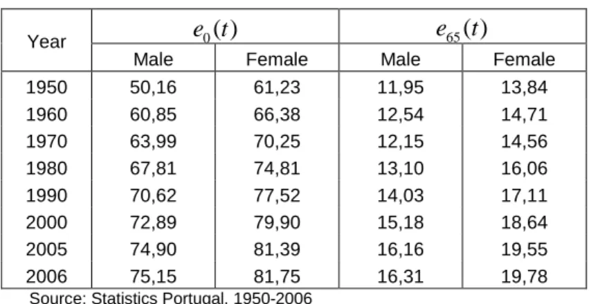
, a major decline in the entropy of the survival curve, a huge increase in the median future lifetime and a significant tightening of the inter-quartile range. All of this confirms the importance of the rectangularization and expansion phenomena in the Portuguese population.3

Table shows the evolution of life expectancy at birth,

e t

₀

( )

, and at age 65,

e

₆₅

( )

t

, over the period 1950-2006. The huge gains in life expectancy are evident for both men and women. Life expectancy at birth increased from 56.2 years for men and 61.2 years for women to 75.2 and 81.8 years, respectively. Men can now expect to live a further 19.0 years and women a further 20.5 years if mortality rates remained as estimated by 2006 life tables. It should be noticed, however, that gains in life expectancy were not uniform over this period, with the most expressive improvements being registered in the first 30 years of this sample. The rate of increase in life expectancy tends to slow down, mainly because future progresses will be achieved primarily by declines in mortality among older segments of the population.

Table 1 – Life expectancy at birth and at 65 years old, Portugal 0

( )

e t

e

65

( )

t

Year

Male Female Male Female

1950 50,16 61,23 11,95 13,84 1960 60,85 66,38 12,54 14,71 1970 63,99 70,25 12,15 14,56 1980 67,81 74,81 13,10 16,06 1990 70,62 77,52 14,03 17,11 2000 72,89 79,90 15,18 18,64 2005 74,90 81,39 16,16 19,55 2006 75,15 81,75 16,31 19,78

Source: Statistics Portugal, 1950-2006

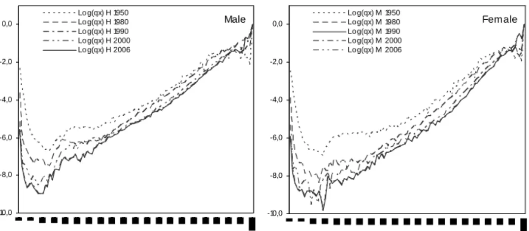
In Figure 3 we represent the mortality rates for a number of selected periods. The mortality hump at young ages, which represents the mortality due to accidents and violent causes of death, tends to spread over and to lose some importance both for men and women. It is represented by probabilities

q

_x particularly significant at ages between 15 and 30 years old, in consequence of the increased risk of violent deaths, most noticeably among the male population. Note also that by age 25-30, mortality follows its inevitable increasing trajectory with age at a more regular rhythm.

Finally, we note that the aged population differs significantly from the general population, others things being equal because of the proportion of women that comprises it. Effectively, even when there is a balanced distribution among male and female new births, gender differences in

3_{The complete set of results is not reported here due to space constraints but can be obtained from the authors upon}

(6)

mortality translate into a preponderance of women at older ages. This proportion increases with age. In Portugal, as in most developed countries, the average gap in life expectancy between the sexes is roughly 6.6 years at birth and 3.5 years at age 65.

Figure 3 – Mortality rates (

x

a

ln(

q

_x

)

_{), Portugal}

Male -10,0 -8,0 -6,0 -4,0 -2,0 0,0 Lo g(qx) H 1950 Lo g(qx) H 1980 Lo g(qx) H 1990 Lo g(qx) H 2000 Lo g(qx) H 2006 Female -10,0 -8,0 -6,0 -4,0 -2,0 0,0 Lo g(qx) M 1950 Lo g(qx) M 1980 Lo g(qx) M 1990 Lo g(qx) M 2000 Lo g(qx) M 2006

3. Data sources

The database used in this study comprises two elements: the observed number of death

d

_{x t}_,

given by age

x

, year of death

t

and, from 1980 onwards, also by year of birth, and population estimates

P

_{x t}_, at December 31 of each year. The data, discriminated by age (

x

∈

[0, 99]

) and sex, refers to the entire Portuguese population and has been supplied by Statistics Portugal. Deaths statistics are based on information collected at death registration by Civil Registration Offices. The declaration of death is a legal requirement, compulsory in Portugal since 1911 and based on official documents. The registry is exhaustive and the data are thought to be reliable, even for old people. However, for the very old some inconsistencies may persist in reporting age due to birth register problems.

The decennial population censuses provide the base figures from which official national resident population estimates for Portugal are derived. The latest census was carried out in 2001. Annual population estimates at 31st December, by age and sex, are obtained by rolling forward the estimates produced after a census using data on subsequent births, deaths and net migration. These rolled-forward estimates are generally subject to increasing error as they move further away from the last census. Population estimates are produced by sex and single year of age up to 99. However, they are officially disclosed only up to age 84, together with total figures for the group aged 85 years and older. This is justified by the fact that these figures may be heavily contaminated by random fluctuations, due to the small number of those surviving up to very old ages as well as to the probable misreporting of ages occurred at the censuses.

(7)

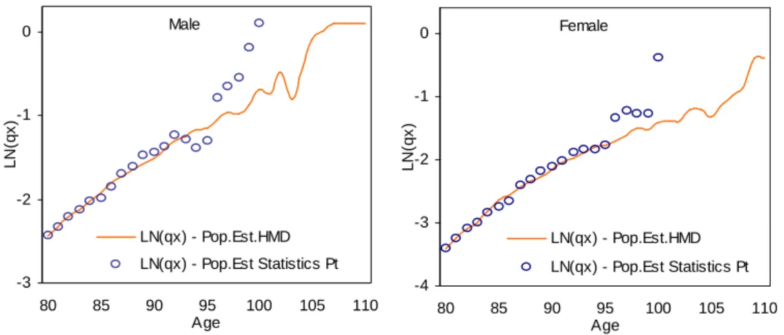
In Portugal, the calculation of crude age specific mortality rates at advanced ages suffers from several problems. The main issue concerns the quality and the availability of data on population estimates for ages 85 and above. Effectively, although data on deaths are in general of good quality, mortality rates may suffer from some inconsistencies at these ages, given that coherence between deaths and the number of those exposed at risk may not exist. Another concern refers to the degree of volatility observed in age-specific mortality rates at very old ages, a feature which affects the statistical significance of the results. To illustrate these problems, Figure 4 represents the mortality rates at age 80 and over for the period 2004-2006 based on official estimates and based on population estimates provided by the Human Mortality Database (HMD). Recall that the later are computed using the methods of extinct generations and almost extinct generations.4

Figure 4 – Mortality rates for the oldest-old

Male -3 -2 -1 0 80 85 90 95 100 105 110 Age L N (q x ) LN(qx) - Pop.Est.HMD LN(qx) - Pop.Est Statistics Pt Female -4 -3 -2 -1 0 80 85 90 95 100 105 110 Age L N (q x ) LN(qx) - Pop.Est.HMD LN(qx) - Pop.Est Statistics Pt

Source: Author’s calculation based on data from Statistics Portugal and Human Mortality Database (www.mortality.org)

Age specific probabilities of death

q

_x are calculated using three-year periods, by pooling deaths and exposures first and then dividing the former by the latter. Consider a two-year birth cohort in the age interval from

x

to

x

+

1

. Let

P

&

denote the sum of the January 1st population estimates for the two individual birth cohorts when they are aged

x

. Likewise, let

D

&

_L and

D

&

_U

denote the sums of lower and upper triangle deaths within the same age interval for the same group of cohorts. Therefore, the probability of death for this two-year cohort is:

4

Recall that the method of extinct generations uses the available information on the number of deaths, by age and year of birth, from the death registrations, to reconstruct the surviving population, without using the census population at all. It is based on the assumption that when all the members of a given generation (people born in a given calendar year) have died, it is possible to reconstruct the numbers who were alive earlier, if the dates of death of everyone in that generation are known. This assumes that international migration can be ignored, which is the case if we confine to ages high enough so the migration flows are negligible. In practice, it is not necessary to wait until all the members of the generations concerned have died. By the time that the members of a generation have reached a given age (e.g. 100 years), only a small proportion of its original members will still be surviving and this proportion, that is, the ratio of the number of survivors who are still living to the members in the generation who died during the last years, can be estimated from the experience of previous generations. Multiplying this "survivor ratio" by the number of deaths that have occurred in a given generation during the last years, it is possible to obtain an estimate of the corresponding number of those who are still alive (survivors). Then, it is possible to reconstruct the past population by adding the estimated number of survivors to the number of registered deaths, generation by generation. This iterative procedure of reconstruction should be calibrated so that the population estimates obtained applying this method coincides with the values of the official organisms for the established maximum age (e.g., 85 years in Portugal).

(8)

L U x L

D

q

P

D

+

=

+

&

(1)

The death rates

m

_x are calculated by first computing the corresponding exposure-to-risk under the assumption that deaths are distributed uniformly within Lexis triangles.5

As we can observe, Figure 4 exhibits visible random fluctuations in mortality rates above age 92 for males and above 95 for females. Moreover, mortality rates based on population estimates calculated according to the method of extinct generations tend to diverge significantly at advanced ages, signalling data problems on official population estimates at these ages. In order to construct complete life tables, it was decided to remove fluctuations by smoothing crude estimates via a projection method.

4. Approaches in estimating mortality rates at advanced ages

4.1. The Coale-Kisker Method

The Coale-Kisker method, named after Coale and Guo (1989) and Coale and Kisker (1990), assumes that the exponential rate of mortality increase at very old ages is not constant, as stipulated by the classical Gompertz model, but declines linearly, a pattern empirically confirmed by the authors of this paper in Portugal and by a number of studies (e.g., Horiuchi and Wilmoth, 1998).6 The Coale-Kisker method establishes that:

max 79 80

exp

x x i i

m

k

=





=







∑



,

80 ≤ ≤

x

max (2)

where

k

_i denotes the rate of mortality increase (defined by

k

_x

=

ln(

m m

_x _x₋₁

)

) at age

x

and max

x

is the highest attainable age considered (110 years in their case). Coale and Kisker (1990) assume that

k

_x is linear above a certain age, 80 years in this case, that is:

(

)

80

x

k

=

k

+ −

x

⋅

s

,

x

≥

80

(3)

In order to determine the slope coefficient

s

, the authors set an arbitrary value for

m

₁₁₀, namely 110

1.0 m

=

for males and

m

₁₁₀

=

0.8

for females. The mortality differential by sex at age 110 was intentionally chosen to avoid a crossover between male and female mortality at advanced ages.

By inserting (3) into (2) and solving for

s

, we obtain

79 110 80

ln(

) 31

465 m

m

k

s

= −

+

(4)

Mortality rates at age 80 and above are finally estimated by:

5

For more details see Wilmoth et al. (2005).

6

Coale and Guo (1989) used this approach to close the extended version of the Coale-Demeny abridged (five-year age groups) model life tables. More specifically, the authors replace observed age specific death rates at old ages (85 years and over) by a sequence of death rates extrapolated for the age groups 85-89, 90–94, ..., 105-109, by assuming that the

(9)

(

)

(

)

79 80 80

exp

80

x x i

m

k

i

s

=





=

_

+ −

⋅

_



∑



,

x

∈

{80,81,...,109}

(5) or simply by:

(

)

1

exp

80

x x

m

=

m

₋

_



k

+ −

x

⋅

s



_

,

x

∈

{80,81,...,109}

(6) The method assumes that the observed death rates around

x

=

80

are reliable and that

k

₈₀

can be calculated from empirical data. In practise, we may need to smooth

k

_x around age 80 to eliminate irregularities. To perceive the influence of the boundary constraint set for the mortality rate at the highest attainable age, we have investigated whether changing the value of

max x

m

modifies our results. Specifically, a number of different versions of the model has been tested

considering

[

]

max

0.8; 0.9; 1.0; 1.1; 1.2; 2.0

x

m

∈

with limit age

x

_max

∈

(110,120)

.

4.2. The method of Denuit and Goderniaux

Denuit and Goderniaux (2005) recently developed a new method based on mortality rates

q

_x

that imposes a closure constraint on life tables. Specifically, the method involves fitting the following log-quadratic regression model:

2

ˆ

ln

q

_x

= + +

a bx cx

+

ε

_x with

ε

_x

~

Nor

(

0,

σ

2

)

(7) to data observed at advanced ages (

x

≥

75

in our case), with the following two constraints:

max

1

x

q

=

(8) max '

0

x

q

=

(9) where max ' x

q

denotes the first derivative of

q

_x with respect to age

x

,

a

,

b

and

c

are parameters to be estimated by OLS and

x

_max is a predefined highest attainable age.

By inserting (8) and (9) into (7), it can be shown that the model can be written as a function of a single parameter, i.e.,

(

2 2

)

max max

ˆ

ln

q

x

=

x

−

2 (

x x

)

+

x

c

+

ε

x with

(

)

2

~

0,

x

Nor

ε

σ

(10)

Constraints (8) and (9) impose a concave shape to mortality rates at advanced ages and the existence of a horizontal tangent at

x

=

x

_max. Constraint (9) aims to prevent an eventual decrease of the mortality rates at very old ages.

To understand the influence of the limit age on the performance of the model, we tested three different versions of (7) considering

x

_max

∈

{110,115,120}

. The final value for

x

_max is chosen to be the one that better describes the data.

(10)

To determine the age above which the original estimates

qˆ

_x should be replaced by the fitted values generated by regression (7), we used an iterative procedure that runs model (7)-(8)-(9) over the age interval

x

∈

[ , 95]

x

₀ , considering different values for

x

₀ (ranging from 70 to 90 years). To determine the “cutting-age

x

₀*”, we used the maximization of the determination coefficient

R

2 as an optimum criterion. The tests carried out allowed us to identify ages 85 and 89 as generating similar values for

R

2, so both have been considered as candidates in the choice process. To prevent the existence of discontinuities in the pattern of mortality rates in the neighbourhood of

x

₀*, and to ensure a smooth transition between the original estimates and the adjusted values, some graduation is normally needed. In our case, we simply replaced initial estimates

qˆ

_x within the age-interval

x

= −

x

*₀

5,...,

x

₀*

+

5

by their five-year geometric average.

4.3. The Logistic Model

The logistic function exhibits an "S" shape, that is, it grows quickly at first and then decelerates its progression, presenting a convenient asymptotic behaviour when it comes to model mortality rates at advanced ages. Formally, the logistic model for the force of mortality can be defined in general terms as (e.g., Thatcher et al., 1998):

(

)

3 3 2 1 2 2 3

1

x x x

e

θ θ

θ

µ θ

_θ

σ

θ

= +

+

−

(11)

where

θ

=

( ,

θ θ θ σ

₁ ₂

,

₂

,

2

)

are parameters to be estimated.

The logistic model has been presented under a number of different versions of (11). In this paper, we adopt first the specification proposed by Perks (1932), defined as:

0 1 2 1 [ ( 80)] 3 [ ( 80)]

1

x x x

e

θ θ θ θ

θ

µ

=

+

₊+ ₋−

+

,

x

≥

80

(12) where

θ

_i

≥

0 (

i

=

0,..., 3)

.

Note that the effect of the denominator in (12) is to flatten out the exponential increase of the Gompertz term in the numerator, noticeable at ages above about 80, which is now a well-established feature of mortality. Assuming that the number of observed deaths follows a Poisson distribution with parameter

µ

_x

E

_x, i.e.,

d

_x

~

Poisson

(

µ

_x

E

_x

)

, where

E

_x denotes the population exposed at risk, it can be shown that parameters

θ

=

( , ,

θ θ θ θ

₀ ₁ ₂

,

₃

)

are estimated by maximizing the following log-likelihood function:

(

)

( )

100 80

ln ( )

x x x

ln

x x

ln

x

!

x

L

θ

E

µ

d

E

µ

d

=

∑



_

−

+

−



_

,

x

≥

80

(13)

(11)

4.4. The Kannistö Model

The model suggested by Kannistö (1992) is another special case of the logistic function, for which the logit transformation of the mortality rate can be express as a linear function of age. In this paper, we test a two-parameter version of the model defined by:

0 1 0 1 [ ( 80)] [ ( 80)]

1

x x x

e

θ θ θ θ

µ

=

+₊ −₋

+

,

x

≥

80

(14)

where

θ

i

≥

0 (

i

=

0,1)

. Note that the model has an asymptote equal to one.

Assuming that the number of observed deaths follows a Poisson distribution with parameter

x

E

x

µ

, i.e.,

d

_x

~

Poisson

(

µ

_x

E

_x

)

, where

E

_x denotes the population (centrally) exposed at risk, parameters

θ

=

( , )

θ θ

₀ ₁ are estimated by maximizing log-likelihood function (13).

5. Results

In this section we describe the results from implementing the approaches in estimating mortality rates at advanced ages described in Section 4. All methods were applied to crude death rates and probabilities

q

_x calculated according to definition (1), for two different periods (2003-05 and 2004-06) and for the three populations under study (men, women, both sexes).7 The results obtained by the different approaches are presented in terms of projected value for

q

_x and in terms of computed estimates for the life expectancy at ages 0, 65, 80, 90 and 100. Finally, the projected values for

q

_x at ages 100, 115 and 120 years old produced by the different methods are reported, in order to perceive the ability of each model to suggest a highest attainable age to be considered when closing the life table. Because of space constraints, we report the results only for the complete population (both sexes).

In Figures 5, 6, 7 and 8 we compare crude estimates of

q

_x with those generated by the different approaches. We can observe that crude estimates of

q

_x at advanced ages (above age 92 for males and above 95 for females) present a rather irregular behaviour, assuming, in some cases, a decreasing trend with age, a profile inconsistent with the expected trajectory for the evolution of the human mortality. In general terms, we note that mortality roughly increases with age, but the rate of mortality increase tends to decelerate from a certain age (85 to 90 years). This pattern translates into a graphical configuration characterized by a clear concave shape for the function

x

a

ln(

q

_x

)

_{, a result that is consistent with the findings of prior empirical studies} on the behaviour of mortality at advanced ages.

The analysis of Figures 5, 6, 7 and 8 highlights that the goodness-of-fit of the alternative methods tested varies significantly. The method proposed by Denuit-Goderniaux (DG) seems to

7

(12)

naturally extend the mortality rates observed at old ages. However, it is clear that the performance of the model is sensitive to both changes in the value of the limit age and of the age above which the original estimates are replaced by fitted values. For this particular population, the closest fit is attained by assuming that

x

_max

=

115

and that crude estimates are replaced by fitted values above age 85. The maximum attainable age considered should not ignore the maximum age for which deaths are registered at that moment in time.

Figure 5: Crude

q

_x and quotients extrapolated by Denuit-Goderniaux method

Age lo g (q x ) 70 80 90 100 110 120 -4 -3 -2 -1 0 crude qx (xmax;xs)=(110-85) (xmax;xs)=(110-89) (xmax;xs)=(115-85) (xmax;xs)=(115-89) (xmax;xs)=(120-85) (xmax;xs)=(120-89)

Notes: xmax = highest attainable age; xs = age above which the original estimates are replaced by the fitted values.

Figure 6: Comparison between crude

q

_x and quotients extrapolated by Coale-Kisker method

Age lo g (q x ) 80 90 100 110 120 -4 -3 -2 -1 0 crude qx m110=0.8 m110=0.9 m110=1.0 m110=1.1 m110=1.2 m120=1.0

(13)

q

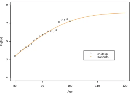
_x and quotients extrapolated by Kannistö model Age lo g (q x ) 80 90 100 110 120 -4 -3 -2 -1 0 crude qx Kannisto

q

_x and quotients extrapolated by Perks model

Age lo g (q x ) 80 90 100 110 120 -4 -3 -2 -1 0 crude qx Perks

The performance of Coale-Kisker (CK) method is quite reasonable but strongly depends on the pre-defined values for the mortality rate corresponding to the limit age

max x

m

and on the limit age itself. Effectively, we note that the arbitrary values for

m

₁₁₀ originally set by CK are not adequate to describe the mortality pattern observed in the Portuguese population. However, it should be stressed that the model is flexible enough to accommodate different mortality

(14)

behaviours, and that by appropriately setting

max x

m

we can replicate the empirical evolution of mortality across age.

The good performance of both DG and CK methods cannot be distanced from the fact that both methods impose constraints to the extrapolation process, which allow us to calibrate the models to the conditions observed at each moment in time, taking into consideration the maximum age for which deaths are registered in the population. The method suggested by Denuit-Goderniaux presents, however, an advantage over Coale-Kisker, since it allows us to set the limit age in advance, that is, gives us the chance to establish beforehand the age at which life tables should be closed. This means that we no longer need to close life tables by setting a probability of death for an open interval at and above

x

_max.

To understand if the closing constraint

max

1

x

q

=

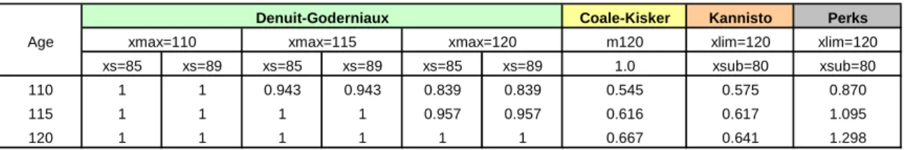
imposed by Denuit and Goderniaux (2005) is reasonable from the point of view of the other models analysed, Table 2 reports the projected values for

q

_x at advanced ages generated by all models. As mentioned before, this is an important issue when it comes to produce complete life tables, and can be seen as an attempt to ascertain the differences between models that impose a closing constraint and models that merely extrapolate mortality rates observed in a given age interval. We note that models which are based on a simple extrapolation procedure convey values for

q

_x that resemble the behaviour of crude estimates up to a certain age, but in contrast produce unreasonable estimates at extreme ages. For example, we observe that the Coale-Kisker and the Kannistö models admit, with a quite high probability, that some members of the population will live beyond age 120.

Table 2: Projected values for

q

_x at advanced ages

HM

Coale-Kisker Kannisto Perks

Age m120 xlim=120 xlim=120

xs=85 xs=89 xs=85 xs=89 xs=85 xs=89 1.0 xsub=80 xsub=80 110 1 1 0.943 0.943 0.839 0.839 0.545 0.575 0.870 115 1 1 1 1 0.957 0.957 0.616 0.617 1.095 120 1 1 1 1 1 1 0.667 0.641 1.298 METHOD Denuit-Goderniaux

xmax=110 xmax=115 xmax=120

On the contrary, in Figures 7 and 8 we observe that the logistic models of Kannistö and Perks basically extrapolate the mortality patterns conveyed by crude estimates, without any control over “natural” and observed mortality trends at old ages. Consequently, models tend to generate unexpected patterns at very old ages, either producing almost constant mortality rates (as it seems to be the case for the Kannistö model), either generating explosive trajectories (as it is the case for the Perks model) that are not confirmed by empirical studies, which show a deceleration in the rate of mortality increase at old ages. The instability of projected values means that the use of logistic models to extrapolate mortality patterns at old ages should be made with caution.

(15)

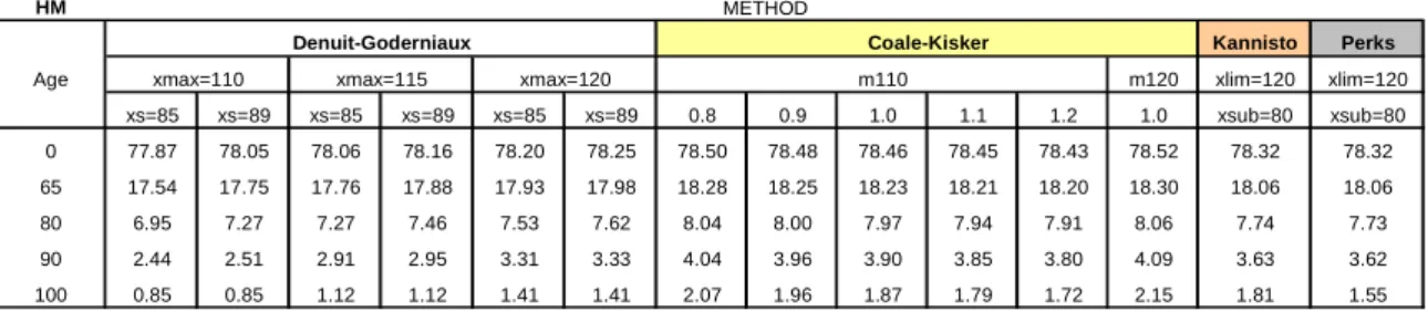
In Table 3 we can analyze the influence of the choice of the method of estimating mortality rates at advanced ages on the values of the complete life expectancy for a selected set of ages, namely

x

∈

{0, 65,80, 90,100}

. The methods proposed by Coale-Kisker, Kannistö and Perks tend to generate higher estimates for the life expectancy at all ages, since they seem to underestimate the evolution of mortality at older ages. The method of Denuit-Goderniaux produces more reliable estimates, and presents a more suitable trajectory for mortality, particularly in the case where the original estimates are substituted by the values adjusted from the 85 years of age. We note also, without surprise, that for the Denuit-Goderniaux method an increase in the highest attainable age translates into higher estimated values for

e

_x at all ages.

Table 3: Estimated life expectancy

e

_x for selected ages (in years) HM

Kannisto Perks

Age m120 xlim=120 xlim=120 xs=85 xs=89 xs=85 xs=89 xs=85 xs=89 0.8 0.9 1.0 1.1 1.2 1.0 xsub=80 xsub=80 0 77.87 78.05 78.06 78.16 78.20 78.25 78.50 78.48 78.46 78.45 78.43 78.52 78.32 78.32 65 17.54 17.75 17.76 17.88 17.93 17.98 18.28 18.25 18.23 18.21 18.20 18.30 18.06 18.06 80 6.95 7.27 7.27 7.46 7.53 7.62 8.04 8.00 7.97 7.94 7.91 8.06 7.74 7.73 90 2.44 2.51 2.91 2.95 3.31 3.33 4.04 3.96 3.90 3.85 3.80 4.09 3.63 3.62 100 0.85 0.85 1.12 1.12 1.41 1.41 2.07 1.96 1.87 1.79 1.72 2.15 1.81 1.55 m110 Coale-Kisker

xmax=110 xmax=115 xmax=120

Denuit-Goderniaux

METHOD

For the Coale-Kisker method, we can observe an inverse relation between

max x

m

and the estimated values for

e

_x. Increasing the age for which

max x

m

is set obviously increases the computed life expectancy.

6. Conclusions

In this paper, we compared the ability of a number of different methods to project mortality for the oldest-old in the Portuguese population in order to establish a sound methodology for the construction of complete life tables. Our results show that models which include a closing constraint seem to be perform better than models that merely extrapolate the mortality patterns observed in a given age interval. The significance of this is that by including closing constraints we no longer need to close life tables by setting a probability of death for an open age interval.

The method suggested by Denuit and Goderniaux presents the best results overall. The method is compatible with recent empirical studies showing that the rate of mortality increase tends to decelerate from a certain age, presenting a concave shape in the (

x

, ln(

q

_x

)

) space, eliminates the possibility of decreasing mortality rates at advanced ages and is flexible enough to accommodate to mortality conditions observed at each moment in time. Future investigations should be able to confirm these conclusions on a broader basis, namely in other countries and for different moments in time.

(16)

References

Boleslawski, L. and Tabeau, E. (2001). Comparing theoretical age patterns of mortality beyond the age of 80. In E. Tabeau et al. (Eds). Forecasting Mortality in Developed Countries: insights from a statistical, demographical and epidemiological perspective. Kluwer Academic Publishers, pp. 127-155.

Bongaarts, J. (2004). Long-Range Trends in Adult Mortality: Models and Projection Methods. Policy Research Division Population Council, Working Paper 192.

Brass, W. (1971). On the scale of mortality. In: Biological Aspects of Demography, London Taylor and Francis.

Buettner, T. (2002). Approaches and experiences in projecting mortality patterns for the oldest-old. North American Actuarial Journal, 6(3), 14-25.

Coale, A. and Guo, G. (1989). Revised regional model life tables at very low levels of mortality. Population Index, 55, 613-643.

Coale, A. and Kisker, E. (1990). Defects in data on old age mortality in the United States: new procedures for calculating approximately accurate mortality schedules and life tables at the highest ages. Asian and Pacific Population Forum, 4, 1-31.

Denuit, M. and Goderniaux, A. (2005). Closing and projecting life tables using log-linear models. Bulletin de l’Association Suisse des Actuaries, 1, 29-49.

Gallop, A. and Macdonald, A. (2005). Mortality at advanced ages in the United Kingdom, Society of Actuaries.

Heligman, L. and Pollard, J. (1980). The age pattern of mortality. Journal of the Institute of Actuaries, 107, 49-80.

Horiuchi, S. and Wilmoth, J. (1998). Deceleration in the age pattern of mortality at older ages. Demography, 35 (4), 391-412.

Kannistö, V. (1992). Development of oldest-old mortality, 1950-1990: Evidence from 28 developed countries. Odense University Press.

Keyfitz, N. (1985). Applied Mathematical Demography. Springer-Verlag, New York.

Lindbergson, M. (2001). Mortality Among the Elderly in Sweden 1988-1997. Scandinavian Actuarial Journal, 1, 79-94.

Olshansky, S. and Carnes, B. (1997). Ever since Gompertz. Demography, 34(1), 1-15.

Perks W. (1932). On some experiments in the graduation of mortality statistics. Journal of the Institute of Actuaries, 63, 12-57.

Pitacco, E. (2004). Survival models in a dynamic context: a survey. Insurance: Mathematics and Economics, 35, 279-298.

Thatcher, A., Kannisto, V. and Vaupel, J. (1998). The force of mortality at ages 80 to 120. Odense Monographs on Population Aging, Odense University Press, Odense.

United Nations (2001). World Population Prospects: The 2000 Revision, Volume I: Comprehensive Tables. New York: United Nations.

Wilmoth, J. (1995). Are mortality rates falling at extremely high ages? An investigation based on a model proposed by Coale and Kisker. Population Studies, 49(2), 281-295.

Wilmoth, J., Andreev, K., Jdanov, D. and Glei, D. (2005). Methods protocol for the Human Mortality Database. Human Mortality Database.