Adjustment of state space models in view of area rainfall estimation

For Peer Review

Adjustment of state space models in view of area rainfall estimation

Journal: Environmetrics Manuscript ID: env-09-0008.R1 Wiley - Manuscript type: Research Article

Date Submitted by the

Author: 24-Feb-2010

Complete List of Authors: Costa, Marco; Universidade de Aveiro, Escola Superior de Tecnologia e Gestão de Águeda

Alpuim, Teresa; Universidade de Lisboa, Departamento de Estatística e Investigação Operacional da Faculdade de Ciências

Keywords: Kalman filter, state space model, parameters estimation, area rainfall estimates

For Peer Review

Adjustment of state space models in view of area rainfall estimation

1 _{Escola Superior de Tecnologia e Gestão de Águeda, Universidade de Aveiro, Apartado 473, 3750-127 Águeda, Portugal}

2 _{Departamento de Estatística e Investigação Operacional, Faculdade de Ciências, Universidade de Lisboa, Edifício C6,}

Campo Grande 1749-016 Lisboa, Portugal

SUMMARY

This paper uses state space models and the Kalman filter to merge weather radar and rain gauge measurements in order to improve area rainfall estimates. Particular attention is given to the estimation of state space model parameters because precipitation data clearly deviates from the normal distribution, and the commonly used maximum likelihood method is difficult to apply and does not perform well. This work is based on 17 storms occurring between September 1998 and November 2000 in an area including part of the Alenquer river hydrographical basin. Based on these data, the work aims to investigate the importance of the parameters estimation method to the accuracy of mean area precipitation estimates. It was possible to conclude that the distribution-free estimation methods produce, in general, better mean area rainfall estimates than the maximum likelihood.

KEY WORDS: Kalman filter; state space model; parameters estimation; area rainfall estimates.

1. INTRODUCTION

Many problems in meteorology and hydrology need an accurate measurement of the total rainfall amount in a certain area. For this purpose, the best results are achieved using both rain gauges and weather radar measurements. However, although rain gauges may provide good point rainfall estimates, they fail to depict the rainfall spatial distribution. Alternatively, weather radar may outline accurate rainfall isopleths (Figure 1), but their point estimates are not so good due to errors of either a meteorological or instrumental nature. This problem can be reduced to some extent if the radar is carefully calibrated. There are several ways to combine the rain gauges and radar estimates taking into consideration the different but complementary nature of the two sensors. Krajewski (1987) and Severino and Alpuim (2005) apply an optimal interpolation method based on Kriging and CoKriging. Calheiros and Zawadzki (1987) and Rosenfeld et al. (1993) use a probability matching method. However, the more commonly used method to merge the radar and rain gauge fields is to relate the two types of measurements through a state space model and consequent application of the Kalman filter.

There are several ways of designing the state space model that relates the gauges observations, the radar observations and their bias. A pioneering work by Ahnert et al. (1986) suggests the relationship

*_{Correspondence to: Marco Costa, Escola Superior de Tecnologia e Gestão de Águeda, Universidade de Aveiro, Apartado 473, 3750-127}

3 4 5 6 7 8 9 10 11 12 13 14 15 16 17 18 19 20 21 22 23 24 25 26 27 28 29 30 31 32 33 34 35 36 37 38 39 40 41 42 43 44 45 46 47 48 49 50 51 52 53 54 55 56 57 58 59 60

For Peer Review

G_t = b_tR_t + e_t, (1)

where Gt and Rt represent the gauges and radar measurements respectively, and bt stands for

the bias or dynamic calibration factor. The measurement error series et is a white noise

sequence with variance σe

2_{. This is called the measurement equation whereas the equation}

governing the time variation of the calibration factor is called the transition equation. Ahnert

et al. (1986) propose that the bias should follow a random walk as it is equally likely to increase or decrease. Alpuim and Barbosa (1999), however, achieve better results in the calibration process using a more general first-order autoregressive, AR(1), process for the transition equation.

FIGURE 1

---Figure 1: Image of the radar surface rainfall intensity field.

Equation (1) describes the relationship between a rain gauge and a radar cell in the same site, but it can be used to produce a mean-field bias, replacing Gt and Rt by the vectors comprising

all the gauges in a certain area and the corresponding radar cells. In this approach Lin and Krajewski (1991) consider a different type of state space model defining the measurement equation as

zt = bt+ et

where zt represents the observed mean bias, that is, the ratio of the sum of all rain gauge data available at time t, over the sum of the corresponding radar data. The study of this model was continued in other works with minor variations in the way the mean-field bias is defined, as may be seen in Anagnostou et al. (1998), Anagnostou and Krajewski (1999) or Chumchean et

al. (2004).

Brown et al. (2001) propose another type of state space model for the combination of the two types of data. These authors make the fundamental assumption that the relationship between gauge and radar reflectance measurements can be described by a power law. Thus, they conclude that there is a linear relationship between Yt = logGtand ut = log Rt that adjusts well to the data if the intercept varies in time as an AR(1) process, that is,

Yt = at + bu + Zt,

where b is constant and Ztis a gaussian white noise process with null mean and variance σZ

2 _.

Without being exhaustive, the models described in the previous paragraphs show that state space models have been extensively used in radar precipitation measurement. The Kalman filter iterative algorithm applies to these models to estimate the bias as its orthogonal projection on the gauge measurements up to time t. This estimator is the minimum mean square error linear predictor which, under the assumption of normality, corresponds to the minimum variance estimator.

In this work we assume that relationship (1) is true and that the calibration factor bt follows an

AR(1) stationary process. Among other possible state space models, we consider this one because it is simple to deal with and reflects the known type of dynamics relating gauge and radar measurements. We focus on the statistical adjustment of models, giving particular attention to the parameter estimation process. The values for the noise variances used in the Kalman filter have a strong influence on the quality of the bias and area rainfall estimates.

4 5 6 7 8 9 10 11 12 13 14 15 16 17 18 19 20 21 22 23 24 25 26 27 28 29 30 31 32 33 34 35 36 37 38 39 40 41 42 43 44 45 46 47 48 49 50 51 52 53 54 55 56 57 58 59 60

For Peer Review

The estimation problem has been addressed since the first works on radar calibration appeared. Ahnert et al. (1986) propose intuitively based estimation methods, but nothing is proved about their statistical properties. Lin and Krajewski (1991) consider an adaptive error estimation parameter algorithm applied to their alternative state space formulation, which Anagnostou et al. (1998) compare with the maximum likelihood applied to the same equations. In many applications, the state space models’ parameters are estimated by maximum gaussian likelihood via the Newton-Raphson method (Harvey, 1996) or, more often, the EM algorithm (Shumway and Stoffer, 1982). However, precipitation data may deviate considerably from the normal distribution and these methods may lead to poor estimates, fact which is also recognized by Anagnostou and Krajewski (1999). Furthermore, the loglikelihood function of state space models with time varying coefficients - as is the case - may have a complex shape which makes it very difficult, or even impossible, to reach the global maximum.

Hence, there is a serious need to find estimation methods with good statistical properties, easy to apply so that they are suitable for real time radar estimation rainfall and flexible enough to adjust to the specific characteristics of rainfall measurements. The main objective of this paper is to use parameter estimators based on the generalized method of moments (GMM) in the radar calibration process. We consider two different estimators of this type, as proposed by Costa and Alpuim (2010) and by Alpuim (1999) and compare them with the maximum likelihood method. The GMM estimators have good statistical properties, and we generalize this method to the case of a multivariate state space model that produces a mean field bias based on several rain gauges in a certain area.

The data available for this study correspond to 17 storms which occurred between September of 1998 and November of 2000 in an area of high hydrometeorological interest located around 40 km north of Lisbon. We use this data to investigate the impact of parameters estimation methods on the accuracy of area precipitation estimates. The authors conclude that GMM estimators have a better performance in mean area rainfall estimation. It is interesting to compare this conclusion with the results in Anagnostou et al. (1998), where adaptive recursive methods involving error correlations compare favorably with maximum likelihood, although applied to different measurement and transition equations. Besides the good results in practice, the proposed GMM estimators are a good alternative to maximum likelihood because they have an analytical expression and are much easier to calculate.

2. DESCRIPTION OF THE DATA

Table 1 describes the data available for this study. They consist of 17 storms between September of 1998 and November of 2000 in a 10x10 km2 area, including the Alenquer River basin, located around 40 km north of Lisbon and between 31 to 44 km distance from the weather radar in Cruz do Leão.

--- TABLE 1 --- --- FIGURE 2 ---

Figure 2: Location of the five rain gauges in the portuguese system of coordinates and in the grid of 25 radar cells used in this work. P – Penedos de Alenquer, A – Abrigada, Mr – Merceana, O – Olhalvo and M – Meca.

3 4 5 6 7 8 9 10 11 12 13 14 15 16 17 18 19 20 21 22 23 24 25 26 27 28 29 30 31 32 33 34 35 36 37 38 39 40 41 42 43 44 45 46 47 48 49 50 51 52 53 54 55 56 57 58 59 60

For Peer Review

There are five rain gauges located in the area being studied, namely, Abrigada (A), Olhalvo (O), Penedos (P), Meca (M) and Merceana (Mr), which correspond to a reasonably high density of gauge/20km2 (see Figure 2). The study area was chosen as the smallest squared grid of radar cells including the five rain gauges available. This choice maximizes the rain gauges density and decreases the errors associated with the interpolation methods. Compared to other works, this area may be considered to have a high density of gauges. For example, Lebel (1999) refers to the network used in the experimental pioneering work by Huff (1970) of 49 gauges spread over a 1000 km2 area, as a dense network. Brown et al. (2001) consider a circular region with an approximate density of one gauge per 500 km2. The area being studied has the highest gauge density under the radar umbrella. This fact, associated with a very low concentration time (about 3h), which makes the region particularly subjected to flash floods, indicates that it is very suitable to conduct radar calibration studies.

The nominal resolution of the radar in Cruz do Leão is 1kmx1km. Nevertheless, as the resolution commonly used in these type of studies is 2kmx2km, we computed the averages of each group of four neighbouring cells. Furthermore, because the original radar data corresponded to 10-minute periods, we used the average of the six available measurements in each hour as the hourly data in each cell of 2kmx2km.

For each cell of 2km×_{2km we have radar rainfall measurements produced by the recently}

installed weather radar in Cruz do Leão, except the storms marked with * in Table 1, where radar measurements are available only in the five cells with rain gauges. The rain gauges in Abrigada and Olhalvo are used to calibrate the radar whereas the remaining three gauges are used to compute the mean area precipitation, usually known as the “ground truth”, in order to assess the quality of the adjusted models. The gauges used for calibration are not used for assessment, since the two processes should be independent. The selection of the two locations for calibration took into consideration the spatial dispersion of the remaining gauges, so that the latter could represent the whole area and the corresponding “ground-truth”.

3. THE KALMAN FILTER ALGORITHM

The Kalman filter technique, Kalman (1960), has been used in many different scientific areas to describe the evolution of dynamic systems. The main goal of the algorithm is to find estimates of unobservable variables based on related observable variables through a set of equations called a state space model. We now describe the two different formulations that will be used to calibrate the radar, in section 6.

The first one considers that in each site where a rain gauge is available the relationship between the gauge, the corresponding radar cell measurement and the bias is described by the set of two equations

Gt = btRt + et (2)

b_t =µ+φ

(

)

|φ| < 1. Also, G_t represents the rain gauge measurement, R_t the radar measurement and e_t

and εt are uncorrelated white noise sequences with variances

2

e

σ and 2

ε

σ , respectively. We will refer to equations (2)-(3) as the multi-factor model because it produces one calibration

4 5 6 7 8 9 10 11 12 13 14 15 16 17 18 19 20 21 22 23 24 25 26 27 28 29 30 31 32 33 34 35 36 37 38 39 40 41 42 43 44 45 46 47 48 49 50 51 52 53 54 55 56 57 58 59 60

For Peer Review

factor at each site where a rain gauge is available. Later, a field of calibration factors is calculated for each radar cell, with the help of interpolation methods.

The second method considers the same radar bias for all the radar cells and will be called the single factor model. This approach uses a multivariate state space model including all radar and gauge measurements simultaneously. Thus, the measurement equation is given by

G_t = b_tR_t + e_t, (4)

where now Gt =[G_1,tG_2,t...Gm_,t]' represents the vector of rain gauges measurements in the m locations at time t, and R_t =[R_1,tR_2,t...R_m,t]' are the correspondent radar observations. In this formulation, the vector of errors et =[e_1,te_2,t...em_,t]' is a multivariate white noise sequence with covariance matrix ΣΣΣΣ_e, which we assume to be diagonal, ΣΣΣΣ_e = diag(σe,1

2 _,...,σ

e,m

2 _{). Hence,}

we suppose that the errors associated with the different gauges are uncorrelated. The state equation is the same as in the multi-factor model, and the white noise sequence of errors εt is uncorrelated with all the components of the measurement error et, that is, E(εtei_,s)=0 for all time instants t and s and for all locations i = 1,…, m.

The multi-factor model is more flexible and, in general, produces more accurate estimates. Seo et al. (1999) call attention to the fact that a single mean field bias cannot generally represent a large area or the entire radar umbrella. However, because of operational constraints and the fact that there are very often large areas with a low density of rain gauges, the single factor approach may be very useful. It has fewer parameters to estimate and may also produce good results when applied to small areas or to storms where the precipitation pattern is spatially homogeneous.

After estimation of the parameters, the Kalman filter may be applied to produce an estimator of the state variable bt, at each time t. This is a recursive algorithm in two steps: the first one

produces a forecast for the next instant calibration factor based on the gauge observations up to time t; the second one updates the forecast taking into account the new gauge observation and the error produced by the calibrated radar. In both steps the bias mean square error is also calculated. This estimator corresponds to the orthogonal projection of the state variable onto the observed variables up to that time. Appendix A summarizes the Kalman filter algorithm. For a more detailed description see Hamilton (1994) or Harvey (1996).

4. ESTIMATION OF THE PARAMETERS

There are several methods that may be used to estimate the state space models parameters. Although the maximum likelihood (ML) method is frequently used, meteorological and hydrological data are, generally, not normally distributed. This will be the case of our data, as may be seen in section 6. This fact, together with the complexity of the ML method for the models in use, shows the need to look for alternative estimation procedures. We present two different distribution-free methods which are based on the generalized method of moments.

4.1 Maximum likelihood estimation of the parameters

Let us consider the case of a single factor state space model, once the likelihood for the multi-factor model is exactly the same with the radar and gauge vectors replaced by the scalar

3 4 5 6 7 8 9 10 11 12 13 14 15 16 17 18 19 20 21 22 23 24 25 26 27 28 29 30 31 32 33 34 35 36 37 38 39 40 41 42 43 44 45 46 47 48 49 50 51 52 53 54 55 56 57 58 59 60

For Peer Review

observations. If the errors are normally distributed, the log-likelihood of the random sample (G₁,G₂,…,G_n) can be written as logL(Θ;G₁,G₂,...,G_n) = −n 2log 2

( )

( )

∑

∑

where Ωt = Rtpt|t −1R ′ t + Σe. Thus, it is possible to obtain the maximum likelihood estimates maximizing the log-likelihood in order to the unknown parameters ΘΘΘΘ = {µ,φ,σ_ε2_,Σ

e} using numerical algorithms, namely, the EM or the Newton-Raphson algorithm.

In our case, the data consist of 17 storms in a total of 178 hours, disconnected in time and therefore can be considered independent. Thus, the log-likelihood is given by the sum of the loglikelihoods for each storm. The use of numerical methods to maximize this likelihood function may be a difficult and complex task, very often without satisfactory results. This problem may occur either because the numerical iterative techniques do not converge or because of the existence of multiple critical points.

4.2 Distribution-free estimation for the parameters – method M1

Costa and Alpuim (2010) propose consistent distribution-free estimators for the parameters of the univariate model (2)-(3) based on the generalized method of moments. These estimators have an explicit analytical expression and do not assume any specific distribution for the errors. They will be designated as M1 estimators.

Considering the multi-factor model as described in equations (2)-(3), the method estimates first the mean of the calibration factor, µ =E[b_t], and then the autoregressive coefficient φ. The estimator for the mean is simply the average of the ratios between the gauges and the radar, that is, ₌ −

∑

t Gt Rt

n 1 ₁

ˆ

µ . The estimator for the autoregressive coefficient is based on

the fact that the autocovariance function for the bias is the same as for the ratios between gauge and radar, that is,

γG/ R(k) = cov Gt +k Rt +k ,Gt Rt     _  = cov bt +k+ et +k Rt +k ,bt + et Rt     _  =γb(k).

Designating by γ(k) this common autocovariance function, as the bias follows an AR(1) process, it verifies the recursive equation

γ

( )

(

)

for any k ≥ 2. Replacing in these equations the autocovariance function by its empirical counterpart,

∑

and considering the first, say, L time lags we can estimate the autoregressive coefficient using the least squares method, i.e., through the minimization of

SQ

( )

(

_{( )}

(

)

)

L

∑

4 5 6 7 8 9 10 11 12 13 14 15 16 17 18 19 20 21 22 23 24 25 26 27 28 29 30 31 32 33 34 35 36 37 38 39 40 41 42 43 44 45 46 47 48 49 50 51 52 53 54 55 56 57 58 59 60

For Peer Review

( )

(

)

∑

(

)

∑

A similar procedure leads to an estimator for the noise variance in the state equation, σ_ε2_,

except that in this case we use the explicit formula for the autocovariance of the b’s process or, equivalently, of the G/R’s process,

γ

( )

for k ≥ 2. Again, replacing γ(k) by the empirical autocovariance and the autoregressive coefficient by ˆ φ as defined by formula (5), we can use the least squares method which leads to the estimator

( )

∑

Finally, note that the estimators for the bias mean and autocovariance are averages calculated over all pairs of observations for which the radar is not null. For the single factor model, the estimation method is the same except that the ratios in all locations have to be considered. Thus, for the estimation of the mean µ, we have =

( ) ∑ ∑

t i t R G nm 1 _{1 1} ˆ µ . The coefficient φ

and the noise variance σ_ε2 _{estimators are given by the same expressions where the empirical}

autocovariance is now the average of the autocovariances over all locations, ˆ γ (k) = 1 nm Gt +k i Rt +k i − ˆ µ     _  Gt i Rt i − ˆ µ     _  i=1 m

∑

∑

After estimating the noise variance for the transition equation we proceed to estimate the variances of the measurement errors, σe,i

2 _{, i = 1,…,m. This is done using the relationship}

Var Gt i Rt i

(

)

( )

which holds in all sites where a rain gauge is available. Hence, equating the average of the square distances of the ratios to µ with its mean value and solving in order to σe,i 2 _{, we get} ˆ σ e2,i= Gt i _R t i_{− ˆ µ}

(

)

∑

( )

∑

These estimators are consistent and compare well with the maximum likelihood, even when the errors distribution is normal (see Costa and Alpuim, 2010). The maximum likelihood method may not converge at all and produces estimates falling outside the parameters space more frequently than this method, especially for small values of the autoregressive coefficient.

4.3 Distribution-free estimation of the parameters – method M2

3 4 5 6 7 8 9 10 11 12 13 14 15 16 17 18 19 20 21 22 23 24 25 26 27 28 29 30 31 32 33 34 35 36 37 38 39 40 41 42 43 44 45 46 47 48 49 50 51 52 53 54 55 56 57 58 59 60

For Peer Review

Alpuim (1999) suggested noise variance estimators for univariate and multivariate state space models, designated in the text by D(k). We need, however, to estimate the autoregressive parameter of the state equation. Thus, in order to apply this method, we combine the D(k) estimators of noise variances with the mean and autoregressive parameters estimators as in method M1. We define the estimation method M2 as the set of noise variance estimators D(k) with mean and autoregressive estimators as in method M1.

To explain this method, let us consider first the univariate model as defined by equations (2)-(3). The D(k) estimators are based on the variables defined by

D k

( )

∑

E D k

[

( )

]

(

)

∑

(

)

∑

Applying the method of moments to these variables, that is, equating the variables D (.) with their mean values for two different indices, say k and l, and solving the resulting system leads to the estimators

) ( ) ( ) ( ) ( ) ( ) ( ) ( ) ( ˆ2 k k k D k D R R R R l l l l Ψ − Ψ − = ε σ and ) ( ) ( ) ( ) ( ) ( ) ( ) ( ) ( ˆ2 k k k D k D Ψ − Ψ Ψ − Ψ = l l l l R R ε σ where _Ψ

( )

k . Usually the indices are taken as k =1 and l=2, but if these

values produce estimates outside the parameters space, other values should be used. This method produces consistent estimators for the noise variances and can be used also in the multivariate state space model. In the case of the single factor model, as defined in equations (3) and (4), each site where a rain gauge is located produces an equation involving σ_ε2 _and

σe,i 2 _{, for i =1,…,m, namely,} D i k

( )

Choosing another index l, any location j and adding the corresponding equation, we have a system of m+1 equations to m+1 unknowns from which the noise variances can be estimated. Costa and Alpuim (2010) show that, in certain conditions, this method leads to estimators with smaller MSE than method M1. They tend, however, to produce estimates outside the parameters space more often than method M1.

5. ASSESSMENT OF THE RADAR-RAIN GAUGE ADJUSTMENT

This section describes how to assess the several models’ performance according to two criteria: point and mean area precipitation. In both cases some of the gauges are used for the estimation and calibration process, whereas the remaining gauges are used to assess the fit of the models. The point precipitation criterion is based on the comparisons of the measurements

4 5 6 7 8 9 10 11 12 13 14 15 16 17 18 19 20 21 22 23 24 25 26 27 28 29 30 31 32 33 34 35 36 37 38 39 40 41 42 43 44 45 46 47 48 49 50 51 52 53 54 55 56 57 58 59 60

For Peer Review

given by each assessment rain gauge with those given by the calibrated radar cell in the same location. Thus, the Error Variance at Gauges (EVG) is given by

EVG =1 n 1 k Gt i_{− ˆ} R t i

(

)

∑

∑

where k is the number of rain gauges, Gt

i _{represents the validation rain gauge at time t and} location i and ˆ R t

i _{= R} t i

bt|t

i _{is the calibrated radar cell measurement correspondent to the same} location.

This criterion has some disadvantages. First, radar and gauge measurements have different natures: while radar represents an area mean value (radar cell), gauges measure precipitation in a point (gauge location). Second, gauges are also subject to errors, although to a smaller extent than radar estimates. However, the EVG can provide some control through the comparison of its value with the estimated variances for the measurement equation.

From the hydrometeorological point of view, mean area estimates are more important than point estimates. While weather radar produces mean area precipitation estimates through an estimated surface of rainfall intensities, gauge provide very poor information on the spatial distribution of precipitation. In this way, a more reliable criterion to assess the models’ performance is based on an estimate of mean area precipitation, known as the “ground-truth”. This is considered to give the best quality pattern because, due to its nature, the true value of mean area precipitation cannot be directly measured. The “ground-truth” is evaluated using interpolation methods in a reasonable thin grid of rain gauges. In general, stochastic interpolation methods, like kriging, are preferable because they provide an estimate for the error. Nevertheless, in our case there are only three validation gauges which are insufficient to estimate a spatial continuity measure, as is needed in the kriging technique. We, therefore, used deterministic methods, namely, Thiessen polygons and the inverse square distance method (ISD), which are commonly used in this type of study (Haberlandt, 2006; Babak and Deutsch, 2008).

The Thiessen polygons method is a simple geometrical process which defines for each gauge an influence area where the precipitation is considered constant and equal to the rain gauge value. In other words, the estimate for each point is its nearest available value in the sense of the euclidian distance.

Alternatively, the inverse square distance interpolation method takes into consideration all available rain gauges to estimate the precipitation in each cell of the grid. In this method, the estimate of the surface function f(⋅) in a point s₀ is the weighted average

ˆ f

( )

( )

∑

∑

where d(s₀,si) is the euclidian distance between the points s0 and si.

After the hourly estimates of the “ground-truth”, GTt, are computed, they are compared with the calibrated radar area rainfall estimates, ARt, through the Root of Mean Square Error (RMSE), that is,

3 4 5 6 7 8 9 10 11 12 13 14 15 16 17 18 19 20 21 22 23 24 25 26 27 28 29 30 31 32 33 34 35 36 37 38 39 40 41 42 43 44 45 46 47 48 49 50 51 52 53 54 55 56 57 58 59 60

For Peer Review

(

)

∑

The calibrated radar area estimate at each time t, ARt, corresponds to the average of the 25 radar cells after calibration, Rˆ =t Rtbt|t. In the multi-factor model, the calibration factors for the grid cells with no rain gauge available are evaluated with the help of an interpolation method. In this work we used also the Thiessen polygons and the inverse square distance methods.

6. RESULTS AND CONCLUSIONS

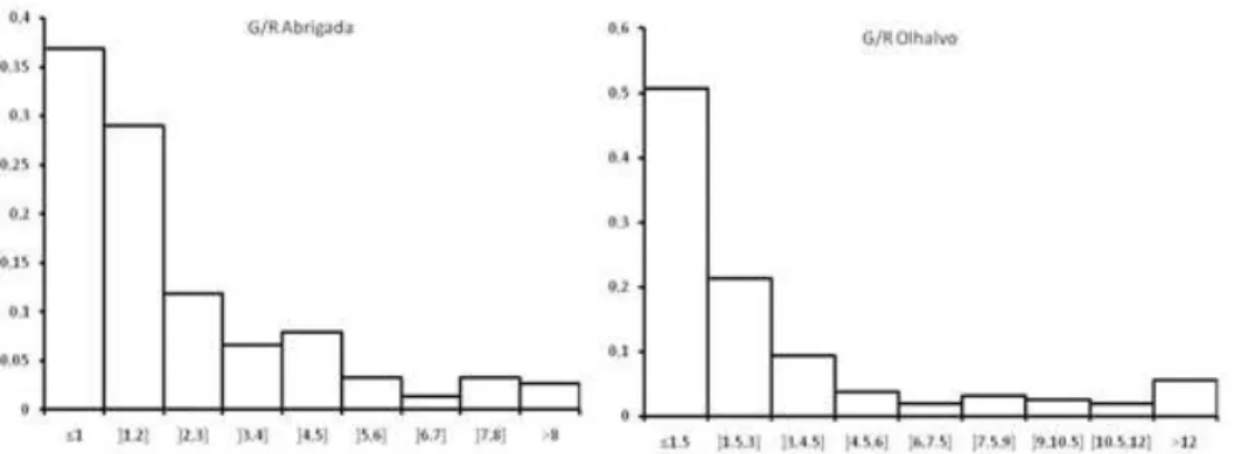
Rain gauges located at Abrigada and Olhalvo were used for the estimation and calibration processes while the remaining gauges were kept for the validation process. Figure 3 plots the ratios gauges/radar at the calibration sites. The analysis of the graphics shows that radar estimates tend to be smaller than the gauges estimates and that these ratios have a great variability. We also observe that the variability of the ratios G/R at Olhalvo is higher than at Abrigada. Figure 4 shows the histogram of G/R data at both locations, reflecting that the bias follows a highly left-skewed probability distribution. The histograms of gauge data are also positively skewed indicating that hour precipitation clearly deviates from the Gaussian distribution. Consequently, we cannot assume that errors in both measurement and transition equations follow a normal distribution. This reinforces the need to look for estimation methods other than the maximum likelihood.

--- FIGURE 3 ---

Figure 3: Plot of ratios of gauges/radar over all storms at Abrigada and Olhalvo.

FIGURE 4

---Figure 4: Histograms of the ratios G/R over all storms at Abrigada and Olhalvo

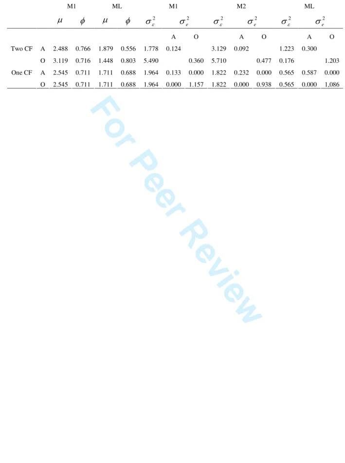
Table 2 presents the results for the model parameters estimation using the three different methods: Gaussian maximum likelihood (ML), the distribution-free methods M1 and M2. These methods were applied both to the single and multi-factor models.

As expected, the estimates for the mean value µ are larger than 1, meaning that the radar underestimates the precipitation when compared to rain gauges. Also, from inspection of figure 3 we may conclude that the ratios G/R at Olhalvo have a large variability, larger than at Abrigada, and this characteristic is reflected in the distribution-free estimates: method M1 produces estimates, both for the mean and the error variance, larger at Olhalvo than at Abrigada. In regard to the means, the maximum likelihood method does not lead to significantly different values at both locations. However, the error variance for the measurement equation at Olhalvo is larger using ML than the distribution-free estimators.

--- TABLE 2 ----

For each combination of model with estimation method, and with the help of the Kalman filter algorithm, we evaluated the bias bt|t, for each hour t at both locations with calibration

gauges. Figure 5 shows the results for the storm of November 2, 2000 where it may be seen

4 5 6 7 8 9 10 11 12 13 14 15 16 17 18 19 20 21 22 23 24 25 26 27 28 29 30 31 32 33 34 35 36 37 38 39 40 41 42 43 44 45 46 47 48 49 50 51 52 53 54 55 56 57 58 59 60

For Peer Review

that all estimation methods improved radar measurements in a similar way. Apparently, there are very small differences between the values produced by methods M1 and M2, but calibrated radar estimates based on ML tend to underestimate rain gauge values in comparison with the other two methods.

--- FIGURE 5 ---

Figure 5: Comparison of rain gauge and radar estimates at Abrigada (top) and Olhalvo (down) with the radar calibrated by the multi-factor model, for the storm of November 2 of 2000.

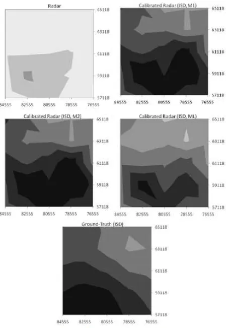
As explained before, after the evaluation of the calibration factors we used Thiessen polygons and the inverse square distance (ISD) interpolation methods to calculate factors for the radar cells where no rain gauge is available. In this way we produce calibration factors for all 25 radar cells. The average of the corrected radar measurements is our mean area precipitation estimate. The analysis of the isopleths of accumulated adjusted radar estimates provides a good appreciation of the final effect of the calibration process. For example, figure 6 compares the accumulated precipitation during the storm of November 2, 2000 using non-calibrated radar estimates, non-calibrated estimates and the “ground-truth”. Analysis of the rainfall maps shows how the calibration process combines radar rainfall spatial distribution with gauge rainfall intensity values. The calibrated radar maintains the rainfall isopleths pattern adjusted to the scale of values given by the rain gauges. Again, maximum likelihood underestimates the accumulated precipitation.

--- FIGURE 6 ---

Figure 6: Accumulated precipitation, in mm, for the storm of November 2 of 2000 for the radar non calibrated estimates and for the calibrated estimates considering the multi-factor model and the three methods of estimation, M1, M2 and ML. Below

we represent the “ground-truth” calculated with the remain locations.

In order to assess the performance of the models, we evaluated the Error Variance at Gauges (point estimation) and the Mean Square Error (mean area estimation) for the calibrated radar series using both one and two factors, with different estimation methods. For the multi-factor model, the two different interpolation methods were compared. Table 3 presents a summary of the final results. It is quite clear that the calibration process leads to a significant error reduction, varying from 19% to 32%, respectively.

--- TABLE 3 ---

The results show that using a calibration factor in each radar cell leads to a higher reduction in the radar bias. Although we are considering a small area within a small distance (approximately 37 km) from the weather radar, it is quite clear that using a different calibration factor for each gauge location improves the final results. However, in each case, we emphasize the importance of balancing the advantages of a more accurate area rainfall estimate with the simplicity and parsimony associated with the single factor model. It is important to note that the reduction in the RMSE achieved with the multi-factor model is not very significant in comparison with the single factor methodology.

In the case of two calibrations factors, the distribution-free estimation methods M1 and M2

3 4 5 6 7 8 9 10 11 12 13 14 15 16 17 18 19 20 21 22 23 24 25 26 27 28 29 30 31 32 33 34 35 36 37 38 39 40 41 42 43 44 45 46 47 48 49 50 51 52 53 54 55 56 57 58 59 60

For Peer Review

When using multiple factors, the maximum likelihood estimation produces the worst results in all cases, although the performance is not very different for the three methods.

When using the same calibration factor for the whole area, the ML method leads to the higher error reduction but shows very similar results to the method M2. Thus, in view of the results achieved in this case study and because of the simplicity of calculation, we much prefer the distribution-free methods. Further, Costa and Alpuim (2010) show, via a simulation study, that the ML method produces more frequently estimates outside the parameters space.

In summary, according to these and previous results, the use of state space models associated with the Kalman filter is an efficient approach to increase the accuracy of weather radar estimation of mean area precipitation. Furthermore, the state space approach allows implementing a real-time process to reduce the radar bias with calibration factors estimated in each time instant. The distribution-free methods are an efficient alternative to the maximum likelihood estimation. In fact, state space models with parameters estimated by these methods can ameliorate substantially the area rainfall estimates. An explanation for this is, probably, that hourly precipitation data deviate considerably from the normal distribution.

Moreover, even in the cases where maximum likelihood shows the best performance, the proposed alternative estimators produce similar results. Thus, it seems clear from these results that the use of distribution-free estimators, easy to apply and with analytical expressions, can achieve similar or better results than the Gaussian maximum likelihood method in the area rainfall estimation problem.

APPENDIX A

The Kalman Filter recursive equations

The Kalman filter is an iterative algorithm that produces an estimator of the state variable bt,

at each time t, which is given by the orthogonal projection of the state variable onto the observed variables up to that time. To simplify ideas let us consider the single-factor model defined by equations (4) and (3). Also, let bt|t-1 represent the estimator of bt based on the

information up to time t−1, that is, based on G1, G2,…, Gt-1, and let pt|t-1 be its mean square error (MSE). As the orthogonal projection is a linear estimator, the predictor for the next variable, Gt, is given by

Gt|t-1= bt|t-1Rt.

When, at time t, Gt is available, the prediction error vector or innovation, ηηηηt = Gt− Gt|t −1, is

used to update the estimate of bt trough the equation

bt|t = bt|t −1+ Ktηηηηt,

where Kt is called the Kalman gain matrix, in this case a 1xm matrix, and is given by K_t = p_{t|t −1}R ′ _t

(

)

Further, the MSE of the updated estimator bt|t verifies the relationship

pt|t = pt|t −1− KtRtpt|t −1.

In its turn, at time t, the forecast for the state vector bt+1 is given by the equation

bt +1|t =µ+φ

(

)

For Peer Review

and it can be easily seen that its MSE is given by p_{t +}1|t =φ 2_p

t|t +σε2.

When using the multi-factor state space model, the same equations apply replacing the radar and gauge vectors of measurements by the scalars Rt and Gt, respectively. This algorithm

produces a real-time correction procedure reducing the radar bias through the combination of the two types of measurements and computes, at each time, the calibration factor bt|t as well as its mean square error pt|t.

References

Ahnert PR, Krajewski WF, Johnson ER. 1986. Kalman filter estimation of radar-rainfall fields bias. In pre-print, 23rd

Conference on Radar Meteorology (3). Boston: AMS, JP33-JP37.

Alpuim T. 1999. Noise variance estimators in state space models based on the method of moments. Annales de l’I.S.U.P.,

XXXXIII (2-3) : 3-23.

Alpuim T, Barbosa S. 1999. The Kalman filter in the estimation of area precipitation. Environmetrics 10: 377-394.

Anagnostou EN, Krajewski W. 1999. Real-Time Radar Rainfall Estimation. Part I: Algorithm Formulation. Journal of

Atmospheric and Ocean Technology 16: 189-197.

Anagnostou EN, Krajewski W, Seo, DJ, Johnson ER. 1998. Mean-field rainfall bias studies for WSR-88D. Journal of

Hydrology Engineering 3(3): 149-159.

Babak O, Deutsch CV. 2008. Statistical approach to inverse distance interpolation. Stochastic Environmental Research and

Risk Assessment 23: 543-553.

Brown P, Diggle P, Lord M, Young P. 2001. Spate-time calibration of radar rainfall data. Applied Statistics 50 (2): 221-241. Calheiros RV. Zawadzki I. 1987. Reflectivity-rain rate relationships for radar hydrology in Brazil. Journal of Climate

Applied Meteorology 26: 118-132.

Chumchean S, Sharma A, Seed A. 2004. Correcting of real-time radar rainfall bias using a Kalman filtering approach. Sixth International Symposium on Hydrological Applications of Weather Radar, Melbourne, Australia.

Costa M, Alpuim T. 2010. Estimation of State Space Model Parameters. To appear in Journal of Statistical Planning and

Inference.

Haberlandt U. 2007. Geostatistical interpolation of hourly precipitation from rain gauges and radar for a large-scale extreme rainfall event. Journal of Hydrology 332: 144-157.

Harvey AC. 1996. Forecasting structural time series models and the Kalman filter. Cambridge University Press: Cambridge. Hamilton JD. 1994. Time Series Analysis. New Jersey: Princeton University Press.

Huff FA. 1970. Sampling errors in measurement of mean precipitation. Journal of Applied Meteorology 9: 35–44.

Kalman RE. 1960. A new approach to linear filtering and prediction problems. Journal of Basic Engineering, Transactions

ASME 82 (series D): 35-45.

Krajewski WF. 1987. Cokriging radar-rainfall and rain gage data. Journal of Geophysical Research 92: 9571-9580.

Lebel T, Amani A. 1999. Rainfall Estimation in the Sahel: What Is the Ground Truth? Journal of Applied Meteorology 38: 555-568.

Lin D S, Krajewski WF. 1991. Recursive methods of estimating radar-rainfall mean bias. Proc., 24rd _{Conference on Radar}

Meteorology, Tallahassee, Florida: AMS, Boston, Mass.

Rosenfeld D, Wolff DB, Atkas 1993. General probability-matched relations between radar reflectivity and rain rate. Journal

of Applied Meteorology 32: 50-72.

Severino JE, Alpuim T. 2005. Spatiotemporal models in the estimation of area precipitation. Environmetrics 16: 773-861. Seo DJ, Breidenbach JP, Johnson ER. 1999. Real-time estimation of mean field bias in radar rainfall data. Journal of

Hydrology 223: 131-147.

Shumway R, Stoffer D. 1982. An approach to time series smoothing and forecasting using the EM algorithm. Journal of

Time Series Analysis 3: 253-264. 3 4 5 6 7 8 9 10 11 12 13 14 15 16 17 18 19 20 21 22 23 24 25 26 27 28 29 30 31 32 33 34 35 36 37 38 39 40 41 42 43 44 45 46 47 48 49 50 51 52 53 54 55 56 57 58 59 60

For Peer Review

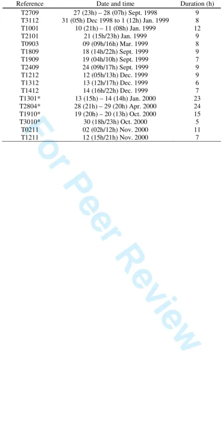
Table 1: Description of the 17 time series used in this application.

Reference Date and time Duration (h)

T2709 27 (23h) – 28 (07h) Sept. 1998 9 T3112 31 (05h) Dec 1998 to 1 (12h) Jan. 1999 8 T1001 10 (21h) – 11 (08h) Jan. 1999 12 T2101 21 (15h/23h) Jan. 1999 9 T0903 09 (09h/16h) Mar. 1999 8 T1809 18 (14h/22h) Sept. 1999 9 T1909 19 (04h/10h) Sept. 1999 7 T2409 24 (09h/17h) Sept. 1999 9 T1212 12 (05h/13h) Dec. 1999 9 T1312 13 (12h/17h) Dec. 1999 6 T1412 14 (16h/22h) Dec. 1999 7 T1301* 13 (15h) – 14 (14h) Jan. 2000 23 T2804* 28 (21h) – 29 (20h) Apr. 2000 24 T1910* 19 (20h) – 20 (13h) Oct. 2000 15 T3010* 30 (18h/23h) Oct. 2000 5 T0211 02 (02h/12h) Nov. 2000 11 T1211 12 (15h/21h) Nov. 2000 7 4 5 6 7 8 9 10 11 12 13 14 15 16 17 18 19 20 21 22 23 24 25 26 27 28 29 30 31 32 33 34 35 36 37 38 39 40 41 42 43 44 45 46 47 48 49 50 51 52 53 54 55 56 57 58 59 60

For Peer Review

Table 2: Estimated values for the parameters for four models at two sites, Abrigada (A) and Olhalvo (O), using the maximum likelihood estimation (ML) and distribution-free estimators (M1 and M2).

M1 ML M1 M2 ML µ φ µ φ 2 ε σ 2 e σ 2 ε σ 2 e σ 2 ε σ 2 e σ A O A O A O A 2.488 0.766 1.879 0.556 1.778 0.124 3.129 0.092 1.223 0.300 Two CF O 3.119 0.716 1.448 0.803 5.490 0.360 5.710 0.477 0.176 1.203 A 2.545 0.711 1.711 0.688 1.964 0.133 0.000 1.822 0.232 0.000 0.565 0.587 0.000 One CF O 2.545 0.711 1.711 0.688 1.964 0.000 1.157 _{1.822 0.000 0.938 0.565 0.000 1,086} 3 4 5 6 7 8 9 10 11 12 13 14 15 16 17 18 19 20 21 22 23 24 25 26 27 28 29 30 31 32 33 34 35 36 37 38 39 40 41 42 43 44 45 46 47 48 49 50 51 52 53 54 55 56 57 58 59 60

For Peer Review

Table 3: Estimates for the RMSE and EVG for the 17 storms. The three estimation methods were combined with the two interpolation algorithms (Thiessen and ISD) both for the evaluation of the calibration factors and the “ground-truth”.

RMSE EVG

Meth. Interp. of the “ground-truth” Thiessen ISD Starting error 1,109 1,120 0,995 Model M. Interp. Meth. Parameter Est.

M1 0.755 0.757 0.807 M2 0.760 0.762 0.804 ISD ML 0.757 0.769 0.843 M1 0.778 0.760 0.817 M2 0.760 0.763 0.816 Two CF Thiessen ML 0.771 0.784 0.853 M1 0,873 0.873 0.826 M2 0.817 0.818 0.806 One CF ML 0.793 0.800 0.817 4 5 6 7 8 9 10 11 12 13 14 15 16 17 18 19 20 21 22 23 24 25 26 27 28 29 30 31 32 33 34 35 36 37 38 39 40 41 42 43 44 45 46 47 48 49 50 51 52 53 54 55 56 57 58 59 60

For Peer Review

Figure 1: Image of the radar surface rainfall intensity field. 158x123mm (96 x 96 DPI) 3 4 5 6 7 8 9 10 11 12 13 14 15 16 17 18 19 20 21 22 23 24 25 26 27 28 29 30 31 32 33 34 35 36 37 38 39 40 41 42 43 44 45 46 47 48 49 50 51 52 53 54 55 56

For Peer Review

Figure 2: Location of the five rain gauges in the portuguese system of coordinates and in the grid of 25 radar cells used in this work. P – Penedos de Alenquer, A – Abrigada, Mr – Merceana, O –

Olhalvo and M – Meca. 96x83mm (96 x 96 DPI) 4 5 6 7 8 9 10 11 12 13 14 15 16 17 18 19 20 21 22 23 24 25 26 27 28 29 30 31 32 33 34 35 36 37 38 39 40 41 42 43 44 45 46 47 48 49 50 51 52 53 54 55 56 57 58

For Peer Review

Figure 3: Plot of ratios of gauges/radar over all storms at Abrigada and Olhalvo. 164x48mm (96 x 96 DPI) 3 4 5 6 7 8 9 10 11 12 13 14 15 16 17 18 19 20 21 22 23 24 25 26 27 28 29 30 31 32 33 34 35 36 37 38 39 40 41 42 43 44 45 46 47 48 49 50 51 52 53 54 55 56

For Peer Review

Figure 4: Histograms of the ratios G/R over all storms at Abrigada and Olhalvo 150x57mm (96 x 96 DPI) 4 5 6 7 8 9 10 11 12 13 14 15 16 17 18 19 20 21 22 23 24 25 26 27 28 29 30 31 32 33 34 35 36 37 38 39 40 41 42 43 44 45 46 47 48 49 50 51 52 53 54 55 56 57 58

For Peer Review

Figure 5: Comparison of rain gauge and radar estimates at Abrigada (top) and Olhalvo (down) with the radar calibrated by the multi-factor model, for the storm of November 2 of 2000.

140x125mm (96 x 96 DPI) 3 4 5 6 7 8 9 10 11 12 13 14 15 16 17 18 19 20 21 22 23 24 25 26 27 28 29 30 31 32 33 34 35 36 37 38 39 40 41 42 43 44 45 46 47 48 49 50 51 52 53 54 55 56

For Peer Review

Figure 6: Accumulated precipitation, in mm, for the storm of November 2 of 2000 for the radar non calibrated estimates and for the calibrated estimates considering the multi-factor model and the three methods of estimation, M1, M2 and ML. Below we represent the “ground-truth” calculated

with the remain locations. 114x163mm (96 x 96 DPI) 4 5 6 7 8 9 10 11 12 13 14 15 16 17 18 19 20 21 22 23 24 25 26 27 28 29 30 31 32 33 34 35 36 37 38 39 40 41 42 43 44 45 46 47 48 49 50 51 52 53 54 55 56 57 58