1 Parte da Tese de Doutorado do primeiro autor, apresentada à USP/ESALQ, com bolsa da Fundect/MS
2 FCA/Universidade Federal da Grande Dourados, C.P. 553, CEP 79804-970, Dourados, MS. Fone: (67) 3410-2415. E-mail: anamarimotomiya@ufgd.edu.br 3 ESALQ/U SP, C.P. 9, CEP 13418-900, Piracicaba, SP. Fone: (19) 3447-8502. E-mail: jpmolin@usp.br
4 D epartamento de Regulamentação, M onsanto do Brasil Ltda, CEP 86600-000, Rolândia, PR. E-Mail: wagner.r.motomiya@monsanto.com 5 Instituto Agronômico, C.P. 28, CEP 13001-970, Campinas SP. Fone (19) 3241-5188, Ramal: 302. E-Mail: sidney@iac.sp.gov.br
Spatial variability of soil properties
and cotton yield in the Brazilian Cerrado
1Anamari V. A. M otomiya2, José P. M olin3, W agner R. M otomiya4 & Sidney R. Vieira5
A BST RA C T
This research aimed at assessing the spatial variability and relationships between factors that affect cotton (Gossypium hirsutum L.) yield. Plant and soil data were collected by a 90 ha area divided in a regular grid of 100 m. In order to detect the variation at small scale, more intense samplings were made with spacing of 33 m, resulting in 5 “ clusters” and totalizing 170 samples. Data were submitted to descriptive statistical analysis, geostatistic and interpolation through ordinary kriging. Variability expressed by the coefficient of variation was from low to moderate for all the variables except for retained bolls and soil P content. Geostatistical analysis indicated that most cotton yield factors presented spatial dependence and this should be considered w hen defining sampling schemes for soil and crop management practices.
Key w ords: geostatistics, nutritional state, spatial dependence
Variabilidade espacial de propriedades do solo
e produtividade do algodoeiro no cerrado brasileiro
RESU M O
O objetivo deste trabalho foi avaliar a magnitude da variabilidade espacial e as relações de causa e efeito entre os fatores de produção da cultura do algodoeiro (Gossypium hirsutum L.). Dados de planta e de solo foram coletados em uma área de 90 ha dividida em malha com espaçamento regular de 100 m entre pontos. Para detectar a variação na pequena escala, amostragens mai s intensas foram fei tas com espaçamento de 33 m, formando 5 “ ilhas” , constituindo o total de 170 amostras. O s dados foram submetidos às análises estatísticas descritivas, geoestatística e interpolação, através de krigagem ordinária. A variabilidade, expressa pelo coeficiente de variação, foi baixa a moderada, para todas as variávei s analisadas, com exceção de maçãs retidas e P no solo. Os resultados da análise geoestatística indicaram que os fatores de produção da cultura do algodoeiro apresentam, em sua maioria, dependência espacial a qual deve ser considerada quando da definição de esquemas de amostragem e práticas de manejo do solo e da cultura.
Palavras-chave: geoestatística, estado nutricional, dependência espacial
Revista Brasileira de
Engenharia Agrícola e Ambiental
v.15, n.10, p.996–1003, 2011
I
NTRODUCTIONThe success of the cotton crop in the cerrado has been driven by favorable weather conditions, topography that allows agricultural mechanization, incentive programs implemented by the government, and especially the intensive use of modern technologies. This latter aspect has meant that the Brazilian cerrado holds the highest yield in cotton crops in Brazil and in the world in non-irrigated areas (EMBRAPA, 2001).
Cotton farms are managed on a very large scale by agricultural enterprises using an intensive production system, totally mechanized to produce high yields. Despite the costs associated with soil fertilization, fertilizers are still applied in a uniform manner over the extremely large fields, without considering soil variability. That also happens in other countries, as observed by Stewart et al. (2005), who verified that USA cotton producers implement extensive management practices on a whole field basis.
The technological evolution in agriculture, however, has demonstrated the importance of measuring spatial and temporal variability of soil properties that affect crop yield (Carvalho et al., 2002; Andrade et al., 2005; Vieira et al., 2007). This information may be used as a basis for implementing application of inputs adjusted site-specifically (Goel et al., 2003, Faria et al., 2009) and some progress also has been done for N variable rate management for cotton (Motomiya et al., 2009). Previous researchers using the theory of regionalized variables have indicated the potential beneût of geostatistics in the agricultural ûelds (Goovaerts, 1999; Viscarra-Rossel et al., 2001).
In this context, the aims of this research were to determine spatial variability and model spatial correlation of the factors that affect cotton yield in a commercial field in the Brazilian Cerrado.
M
ATERIALAND METHODSThe study field is located on a farm called “Planalto”, Chapadão do Céu county, Goiás, Brazil (52o 41’ W; 18o 28’ S).
The field has been managed with annual crops [soy bean
(Glycine max (L.) Merr.), corn (Zea mays L.) and cotton
(Gossypium hirsutum L.)] in rotation. Soil is plowed after cotton
harvest to incorporate cotton stalks in order to control insects. Pearl millet (Pennisetum americanum L.) is used as a crop to produce straw. The soils are classified as the DYSTROPHIC RED OXISSOL, with medium texture with 540, 80 and 380 g dm-3
of clay, sand and silt, respectively on an average altitude of 814 m, predominantly leveled, with slopes varying from 1 to 2%.
Cotton sowing was done in november 25th 2003, using the
DeltaPine Acala 90 cultivar, with 0.90 m row spacings. Soil fertilization was accomplished based on soil analysis, in a uniform manner, for a yield expectation of 4,500 kg ha-1, applying
130 kg N ha-1, 40 kg P ha-1 and 123 kg K ha-1. Insects, diseases
and weeds were controlled based on their occurrence, according to technical recommendations for the region (EMBRAPA, 2001).
Data was collected in a rectangular 90 ha area (1000 x 900 m), divided in a regular grid of 100 m (Figure 1). Two lines of 2.0 m, constituting a sample cell of 3.6 m2, composed each sampling
point. In order to detect variation at smaller scale, some samples were collected at a closer spacings (33 m) in five clusters resulting in a total of 170 samples.
0 100 200 300 400 500 600 700 800 900 1000
X (m) 0
100 200 300 400 500 600 700 800 900
Y
(
m
)
Figure 1. Sampling scheme of the experimental area showing a regular grid and five densely-spaced clusters
Leaf samples were collected at flowering time, between 80 to 90 days after the emergence, composed of 20 upper-most fully expanded leaves, collected on 20 plants by point. Samples were dried and grounded in order to get an analytical determination of nutrient concentrations. Nitrogen was extracted by hot sulfuric digestion and determined by the semi-micro-Kjeldahl method. The nutrients P, K, Ca, Mg, S were extracted by nitric-perchloric hot digestion and determined by colorimetry (P), spectrophotometry flame emission (K), atomic absorption spectrophotometry (Ca, Mg) and barium sulfate turbidimetry (S) (EMBRAPA, 1999).
Cotton yield data was obtained by manually harvesting at each sample point (the area of 3.6 m2). The number of plants,
plant height, open cotton bolls and the number of bolls were also counted during the harvest. Soil sampling occurred immediately after harvesting. Determinations of pH and H + Al, Ca, Mg, K, and Al were determined according to EMBRAPA (1999). After air-drying and sieving (2 mm), the pH was determined in a 0.01 mol CaCl2 L-1 solution. Exchangeable Ca,
Mg, and Al were extracted with a 1 mol KCl L-1 while H + Al with
a 0.5 mol calcium acetate (pH 7.0) L-1. The concentrations of Al
and H + Al were determined by titration using a standard 0.025 mol NaOH L-1 solution. Exchangeable Ca and Mg were
All data was submitted to statistical analysis to determine average, maximum and minimum, skewness and kurtosis coefficients, coefficient of variation (CV) and frequency distribution. The analysis of spatial dependence was conducted by fitting a model to the experimental semivariograms, following the regionalized variables theory, using the software GEOST (Vieira et al., 2002). Vendrusculo et al. (2004) recommended the jack-knifing auto validation procedure to verify the error of estimation in parameters of the models fitted. In this technique, each measured value is interpolated using the kriging method, and the estimated value is successively eliminated during calculation, then an errors study is performed, and it is possible to estimate values with different models fitted to the semivariograms. This technique can be compared to a sen sitivity an alysis of th e fitted par ameter s to th e semivariogram. Once spatial dependence was verified, kriging was performed to estimate values for the non-sampled locations, without bias and with minimum variance. Finally, thematic maps of the spatial distribution of the studied variables were generated.
R
ESULTSANDDISCUTIONTable 1 displays the results of the descriptive statistical analysis of cotton yield and other crop characteristics. Yields varied from 2,843 to 5,704 kg ha-1 and the average yield was
higher than the local average (4,500 kg ha-1). The plant
population averaged 122,600 plants ha-1, varying from 77,800
to 155,600 plants ha-1. Despite this, the CV was low (12.7%).
EMBRAPA (2001) recommend a plant population between 80,000 to 120,000 plants ha-1 for the Cerrado region for currently
used cultivars.
On average, 0.22 healthy bolls were retained and 1.23 rotten bolls were observed per plant, after harvest. According to EMBRAPA (2001), more than 100 species of microorganisms h ave been isolated fr om rotten bolls. Most of th ese microorganisms are secondary pathogens and they act under fruit stress conditions. Some pathogens are primary pathogens and directly infect bolls and cotton squares, causing rotting.
Cotton yield CV was 11.6%, which were similar to the CV values reported by Elms et al. (2001) and Ping et al. (2004) in a cotton ûeld. The retained bolls displayed a quite high CV (97.4%) while other yield component variables showed a CV from low to moderate, according to Wilding & Drees (1983).
Macronutrient concentration in cotton leaves at flowering (Table 1) showed that the average was within sufficiency r an ges. Th e con cen tr ation of N was sligh tly above recommended sufficiency ranges. In spite of the wide range of maximum and minimum values for the different nutrients, all of them displayed a low CV (< 15.0%).
Between the soil properties, K, sum of bases, CEC, base saturation, clay and silt presented a normal distribution, according Kolmogorov-Smirnov test. The others presented large values for the skewness and kurtosis coefficients, which indicate the non-normality of the data. With the exception of H+Al and clay, all variables displayed a positive skewness.
N - observation number; CV - coefficient of variation; CS - coefficient of skew ness; CK - coefficient of kur tosis; d - normal test; ns - non significant by Kolmogorov- Smirnov test
Variable N average Median variance CV(%) minimum maximum CS CK d
Crop characteristics
Height (m) 170 1.2 1.2 0.0082 7.5 0.9 1.5 -0.16 1.11 0.05ns
Stand (pl ha-1
) 170 122663 123611 0.23E+ 09 12.3 77780 155600 -0.36 0.15 0.06ns
Rotten bolls 170 1.2 1.2 0.16 32.9 0.5 2.7 0.87 1.11 0.08ns
Retained bolls 170 0.2 0.2 0.046 97.4 0.0 1.1 1.24 1.47 0.07ns
Open bolls 170 7.2 7.2 1.46 16.8 4.5 12.1 0.84 2.16 0.09ns
Yield (kg ha-1
) 170 4.637 4.654 290.2 11.6 2.843 5.704 -0.64 0.71 0.06ns
Leaf nutrients concentrations
N (g kg-1
) 170 46.9 46.8 12.58 7.6 34.0 61.0 0.91 4.40 0.12
P (g kg-1
) 170 2.7 2.7 0.10 11.7 1.8 3.9 -0.061 0.97 0.11
K (g kg-1) 170 19.3 19.0 4.92 11.5 14.5 28.0 0.65 1.30 0.11
Ca (g kg-1) 170 26.4 26.1 9.60 11.7 19.3 36.8 0.44 0.26 0.08ns
Mg (g kg-1
) 170 3.9 4.0 0.34 14.8 2.5 5.7 -0.073 0.47 0.87ns
S (g kg-1
) 170 6.4 6.3 0.79 13.8 4.6 9.6 1.16 2.21 0.11
Soil properties
pH (H2O) 169 5.6 5.6 0.03 3.1 5.3 7.0 3.53 24.63 0.22
pH (CaCl2) 169 4.9 4.9 0.04 4.2 4.5 6.5 3.05 21.62 0.21
Ca (cmolc dm-3) 169 3.4 3.4 0.29 15.7 2.4 7.5 2.75 19.63 0.12
Mg (cmolc dm
-3
) 169 1.0 1.0 0.05 22.3 0.6 1.8 0.42 0.23 0.14
H_Al (cmolc dm
-3
) 169 6.5 6.5 1.33 17.7 1.8 9.4 -0.29 1.70 0.10
K (cmolc dm-3) 169 0.33 0.32 0.004 20.3 0.19 0.58 0.78 1.15 0.09ns
P (mg dm-3
) 169 21.7 19.6 70.17 38.6 11.3 69.3 2.93 11.57 0.18
Bases(cmolc dm
-3
) 169 4.8 4.7 0.57 15.8 3.2 9.4 1.51 7.86 0.08ns
CEC(cmolc dm-3) 169 11.3 11.2 0.67 7.3 8.2 13.5 0.10 0.69 0.07ns
CECef (cmolc dm-3) 169 4.8 4.7 0.54 15.3 3.3 9.4 1.60 8.38 0.11
Base saturation 169 42.3 42.0 58.09 18.0 27.0 84.0 1.19 4.81 0.10ns
Clay (g kg-1
) 169 540 542 511.0 4.2 446 577 -1.08 2.06 0.10ns
Silt (g kg-1) 169 381 380 511.3 5.9 324 453 0.74 1.30 0.08ns
Sand (g kg-1
) 169 79 78 100.5 12.7 59 130 2.03 7.92 0.14
The lowest values of CV were observed for pH, clay, silt and CEC (CV < 8.0%) and the highest ones for P, Mg, K and base saturation (CV > 18.0%).
Results from the geostatistical analysis are presented in Table 2. Models were fitted to the experimental semivariograms using the best-adjusted model with a smaller root mean square (RMS) and validated by the jack-knifing method (Vendrusculo et al., 2004; Vieira et al., 2010). The number of rotten bolls and open bolls presented a pure nugget effect (absence of spatial dependence in the sampling spacing used). The other crop characteristics were fitted to the spherical model.
The nugget effect (C0) represents non-explained variance, frequently caused by errors in measurement or by variations of properties not detected in the sampling scale (Vendrusculo et al., 2004). Cambardella et al. (1994) proposed that spatial dependence degree (SDD) be verified by the relationship between the nugget effect (C0) and the sill (C0+C) being classified as weak for values greater than 75%; moderate between 25 and 75%; and strong less than 25%. According to this approach, crop variable presented moderate SDD.
The range defines the maximum radius from which neighboring samples are drawn for interpolation by kriging, since samples are spatially related (Vendrusculo et al., 2004). The closerthe samples are, the more important they are in the interpolation and, because of that, the semivariograms must be more accurate, specially at small distances (Vieira et al., 2010). The range is also important for planning and experimental evaluation and can aid in defining the sampling procedure.
Range values of spatial dependence for crop characteristics varied from 174 m for retained bolls to 234 m for cotton yield.
Phosphorus, K and Mg concentrations in leaf tissue presented pure nugget effect, while N was fitted to the Gaussian model and presented weak SDD; Ca and S concentrations in leaf tissue were adjusted to the spherical model with moderate SDD. Oliveira et al. (2009) also fitted the spherical model to N, P, K, Ca and Mg concentrations in citrus leaf tissue. In soil, P, Mg, clay and silt contents did not present spatial dependence. Calcium and sand presented strong SDD, and the other variables presented moderate SDD. Silva & Chaves (2001) observed strong SDD to soil K and P.
According to Cambardella et al. (1994), variables that present strong spatial dependence are more influenced by intrinsic soil properties, such as texture and mineralogy, while those that present weak dependence are influenced by such extrinsic soil properties as fertilizer applications and cultivation, meaning that they are management dependent.
As pointed out by Corá & Beraldo (2006), many precision agriculture consultants in Brazil do not take into consideration spatial dependence of properties to estimate values during the field mapping procedure. They use methods based on linear interpolation or polynomials, which reduce the accuracy of management maps. However, Han et al. (1994) pointed out that the appropriate sample spacing depends on spatial variability and that the sampling scheme can vary between fields. Considering the range of values for soil properties, such as base saturation, it is observed that, for liming site specific
C0 - nugget effect; C
1 - structural variance; r - range; R
2 - coefficient of determination; RMS - root mean square; SDD - spatial dependence degree
Variable Model C0 C1 a R2 RM S GDE
Crop characteristics
Height (m) Spherical 0.005 0.002 200.00 0.64 0.0009 0.68
Stand (pl ha-1
) Pure Nugget Effect
Rotten bolls Pure Nugget Effect
Retained bolls Spherical 0.019 0.025 174.92 0.58 0.010 0.43
Open bolls Pure Nugget Effect
Yield (kg ha-1
) Spherical 182479.89 77843.35 234.65 0.50 49231.90 0.70
Leaf nutrients concentrations
N Gaussian 9.908 2.807 269.45 0.43 3.268 0.78
P Pure Nugget Effect
K Pure Nugget Effect
Ca Spherical 4.576 2.615 194.33 0.45 2.117 0.64
Mg Pure Nugget Effect
S Spherical 0.635 0.233 319.57 0.35 0.231 0.73
Soil properties
pH(H2O) Spherical 0.014 0.012 127.65 0.20 0.004 0.54
pHCaCl2 Spherical 0.015 0.023 127.65 0.33 0.005 0.40
Ca Spherical 0.017 0.243 124.48 0.44 0.038 0.06
Mg Pure Nugget Effect
H+ Al Spherical 0.023 0.031 50.00 0.07 0.004 0.42
K Spherical 0.003 0.001 200.00 0.10 0.001 0.63
P Pure Nugget Effect
SB Spherical 0.191 0.342 118.54 0.48 0.052 0.36
CEC Spherical 0.278 0.440 199.51 0.66 0.083 0.39
CEC ef Spherical 0.198 0.305 119.72 0.44 0.051 0.39
Base saturation Spherical 21.634 33.487 74.32 0.35 4.251 0.39
Clay Pure Nugget Effect
Silt Pure Nugget Effect
Sand Gaussian 0 85.000 136.60 0.47 18.591 0.00
A. B.
0 100 200 300 400 500 600 700 800 900 1000
X (m) 0
100 200 300 400 500 600 700 800 900
Y
(
m
)
4000 4250 4500 4750 5000
0 100 200 300 400 500 600 700 800 900 1000
X (m) 0
100 200 300 400 500 600 700 800 900
Y
(
m
)
0.0 0.2 0.4 0.6
C. D.
0 100 200 300 400 500 600 700 800 900 1000
X (m) 0
100 200 300 400 500 600 700 800 900
Y
(
m
)
1.11 1.16 1.21 1.26 1.31
0 100 200 300 400 500 600 700 800 900 1000
X (m) 0
100 200 300 400 500 600 700 800 900
Y
(
m
)
43.5 45.1 46.7 48.3 49.9
E. F.
0 100 200 300 400 500 600 700 800 900 1000
X (m) 0
100 200 300 400 500 600 700 800 900
Y
(
m
)
21.5 23.5 25.5 27.5 29.5
0 100 200 300 400 500 600 700 800 900 1000
X (m) 0
100 200 300 400 500 600 700 800 900
Y
(
m
)
5.6 6.0 6.4 6.8 7.2
Figure 2. Spati al distribution maps of crop characteristi cs (A) yield; (B) retained boll s; (C) hei ght; and nutritional state: (D) leaf tissue N ; (E) leaf ti ssue Ca; (F) l eaf tissue S
management, samples should be collected with a grid of 74 x 74 m or one sample for each 0.5 ha.
Silva et al. (2007), analyzing the variability of soil properties in a coffee (Coffea arabica L.) field, stated that extrinsic variability related to soil management practices, contributed to range reduction. Therefore, input applications under fixed rates tend to increase variability. Chaves & Farias (2009), evaluating the maps of spatial distribution of copper and manganese prior to application of a sugarcane vinasse and filter cake, concluded
that maps are useful to monitoring the behavior of these elements.
Variable rate applications of inputs like lime and fertilizers decrease variability, resulting in higher range values. In fact, Corá & Beraldo (2006) observed an increase in spatial continuity (wider range) of properties after applying lime and P with variable rates. In two fields, soil P levels presented higher range values after variable application of P, indicating wider spatial continuity of soil P.
Bronson et al. (2003) observed in two irrigated cotton fields that the response to P fertilizer application was not consistent in a study that compared variable rate, fixed rate and lack of P
application. In spite of that, the study revealed that in two of the three experiments, less P fertilizer was required using variable rate application than recommended fixed rate; and landscape position and soil type (calcareous and no-calcareous soil) impacted the response to P fertilizer.
The parameters of the models fitted to the semivariograms were used to spatial distribution maps for the studied variables. Despite the short range between the interpolated values, Figure 2D to 2F show that there are similarities between maps for N, Ca and S in leaf tissue. There is a strip crossing the whole field
A. B.
C. D.
E. F.
0 100 200 300 400 500 600 700 800 900 1000
X (m) 0
100 200 300 400 500 600 700 800 900
Y
(
m
)
4.6 4.8 5.1 5.3 5.6
0 100 200 300 400 500 600 700 800 900 1000
X (m) 0
100 200 300 400 500 600 700 800 900
Y
(
m
)
2.4 3.3 4.2 5.1 6.0
0 100 200 300 400 500 600 700 800 900 1000
X (m) 0
100 200 300 400 500 600 700 800 900
Y
(
m
)
0.26 0.30 0.34 0.38 0.42
0 100 200 300 400 500 600 700 800 900 1000
X (m) 0
100 200 300 400 500 600 700 800 900
Y
(
m
)
3.6 4.5 5.4 6.3 7.2
0 100 200 300 400 500 600 700 800 900 1000
X (m) 0
100 200 300 400 500 600 700 800 900
Y
(
m
)
9.8 10.4 11.0 11.6 12.2
0 100 200 300 400 500 600 700 800 900 1000
X (m) 0
100 200 300 400 500 600 700 800 900
Y
(
m
)
3.8 4.6 5.4 6.2 7.0
A. B.
0 100 200 300 400 500 600 700 800 900 1000
X (m) 0
100 200 300 400 500 600 700 800 900
Y
(
m
)
28 36 44 52 60
0 100 200 300 400 500 600 700 800 900 1000
X (m) 0
100 200 300 400 500 600 700 800 900
Y
(
m
)
55 73 91 109 127
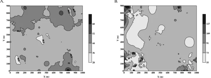
Figure 4. Spatial distribution maps of soil properties: (A) base saturati on; (B) sand
in the Y direction, going from 0 to 600 m in X, where the highest values of these variables are observed. In the same way, cotton yield, retained bolls and plant height presented a similar distribution as leaf elemental concentrations.
Of all the soil properties (Figures 3 and 4), pH (CaCl2), Ca, SB, CECef and base saturation, presented similar spatial distribution, as a result of interdependence between these variables. There is a small spot, in the area between the coordinates 700-900 m X and 0-100 m Y, where elevated values of these variables are concentrated, probably caused by lime deposition before application. When analyzing base saturation variability (Figure 4), with values predominantly between 36 and 52%, we noticed that variable rate liming application could reduce costs and improve the availability of other nutrients for the plants.
Although soil K (Figure 3C) presented medium levels in the area, its spatial distribution suggests variable rate applications would be economically beneficial.
C
ONCLUSIONS1. The variability expressed by the coefficient of variation was predominantly low to moderate for all analyzed variables. 2. Geostatistical analysis indicated that cotton nutrient status and yield, sand, and soil chemical properties showed spatial dependence, indicating that spatial variation should be considered when planning sampling for soil and crop management practices.
3. Leaf tissue concentrations of N, Ca and S, display the same arrangement of spatial distribution along the field.
L
ITERATURE CITEDAndrade, A. R. S.; Guerrini, I. A.; Garcia, C. J. B.; Katez, I.; Guerra, H. O. C. Variabilidade espacial da densidade do solo sob manejo da irrigação. Ciência e Agrotecnologia, v.29, p.322-329, 2005.
Bronson, K.; Keeling, W.; Booker, J. D.; Chua, T.; Wheeler, T.; Boman, R.; Lascano, R. Influence of landscape position, soil series, and phosphorus fertilizer on cotton lint yield. Agronomy Journal, v.95, p.949–957, 2003.
Cambardella, C. A.; Moorman, T. B.; Nowak, J. M.; Parkin, T. B.; Karlen, D. L.; Turco, R. F.; Konopka, A. E. Field-scale variability of soil properties in central Iowa soils. Soil Science Society of America Journal, v.58, p.1501-1511, 1994. Carvalho, J. R. P.; Silveira, P. M.; Vieira, S. R. Geoestatística na
determinação da variabilidade espacial de características químicas do solo sob diferentes preparos. Pesquisa Agropecuária Brasileira, v.37, p.1151-1159, 2002.
Chaves, L. H. G.; Farias, C. H. A. Variabilidade espacial de cobre e manganês em Argissolo sob cultivo de cana-de-açúcar. Revista Ciência Agronômica, v.40, p.211-218, 2009. Corá, J. E.; Araújo, A. V.; Pereira, G. T.; Beraldo, J. M. G.
Variabilidade espacial de atributos do solo para adoção do sistema de agricultura de precisão na cultura de cana-de-açúcar.Revista Brasileira de Ciência do Solo, v.28, p.1013-1021, 2004.
Corá, J. E.; Beraldo, J. M. G. Variabilidade espacial de atributos do solo antes e após calagem e fosfatagem em doses variadas na cultura de cana-de-açúcar. Engenharia Agrícola, v.26, p.374-387, 2006.
Elms, K. M.; Green, C. J.; Johnson, P. N. Variability of cotton yield and quality. Communications in Soil Science and Plant Analysis, v.32, p.351–368, 2001.
EMBRAPA - Empresa Brasileira de Pesquisa Agropecuária. Manual de análises químicas de solos, plantas e fertilizantes. Brasília: Comunicação para Transferência de Tecnologia, 1999. 370p.
EMBRAPA - Empresa Brasileira de Pesquisa Agropecuária. Algodão: tecnologia de produção. Dourados: Embrapa Agropecuária Oeste, 2001. 296p.
Goel, P. K.; Prasher, S. O.; Landry, J. A.; Patel, R. M.; Bonnell, R. B.; Viau A. A.; Miller, J. R. Potential of airborne hyperspectral remote sensing to detect nitrogen deficiency and weed in festation in cor n. Computers and Electr onics in Agriculture, v.38, p.99-124, 2003.
Goovaerts, P. Geostatistics in soil science: state-of-the-art and perspective. Geoderma, v.89, p.1-45, 1999.
Han, S.; Hummel, J. W.; Goering, C. E.; Cahn, M. D. Cell size selection for site-specific crop management. Transactions of the ASAE, v.37, p.19-26, 1994.
Motomiya, A. V. A., Molin, J. P., Chiavegato, E. J. Utilização de sensor óptico ativo para detectar deficiência foliar de nitrogênio em algodoeiro. Revista Brasileira de Engenharia Agrícola e Ambiental, v.13, p.137-145, 2009.
Oliveira, P. C. G.; Farias, P. R. S.; Lima, H. V.; Fernandes, A R.; Oliveira, F. A.; Pita, J. D. Variabilidade espacial de propriedades químicas do solo e da produtividade de citros na Amazônia Oriental. Revista Brasileira de Engenharia Agrícola e Ambiental, v.13, p.708-715, 2009.
Ping, J. L.; Green, C. J.; Zartman, R. E.; Bronson, K. F. Exploring spatial dependence of cotton yield using global and local autocorrelation statistics. Field Crops Research, v.89, p.219-236, 2004.
Silva, F. M.; Souza, Z. M.; Figueiredo, C. A. P.; Marques Júnior, J.; Machado, R. V. Variabilidade espacial de atributos químicos e de produtividade na cultura do café. Ciência Rural, v.37, p.401-407, 2007.
Silva, P. C. M.; Chaves, L. H. G. Avaliação e variabilidade espacial de fósforo, potássio e matéria orgânica em Alissolos. Revista Brasileira de Engenharia Agrícola e Ambiental, v.5, p.431-436, 2001.
Stewart, C.; Boydell, B.; Mcbratney, A. Precision decisions for quality cotton: a guide to site-specific cotton crop management. Sidney: University of Sydney, 2005. 107p. Vendrusculo, L. G.; Magalhaes, P. S. G.; Vieira, S. R.; Carvalho,
J. R. P. Computational system for geostatistical analysis. Scientia Agricola, Piracicaba,v.61, p.100-107, 2004. Vieira, S. R.; Carvalho, J. R. P.; González, A. P. Jack knifing for
semivariogram validation. Bragantia, v.69, p.97-105, 2010. Vieira, S. R.; Millete, J. A.; Topp, G. C.; Reynolds, W. D.
Handbook for Geostatistical analysis of variability in soil and meteorological paramaters. In: Tópicos em Ciência do Solo. v.2. Alvarez, V. H (ed). Viçosa: Sociedade Brasileira de Ciência do Solo, 2002. 45p.
Vieira, V. A. S.; Mello, C. R.; Lima, J. M. Variabilidade espacial de atributos físicos do solo em uma microbacia hidrográfica. Ciência e Agrotecnologia, v.31, p.1477-1485, 2007.
Viscarra-Rossel, R.A.; Goovaerts, P.; McBratney, A.B. Assessment of the production and economic risks of site-speciûc limiting using geostatistical uncertainty modeling. Environmetrics, v.12, p.699-711, 2001.