www.scielo.br/aabc
Scattering of electromagnetic plane waves by a buried vertical dike
LURIMAR S. BATISTA1 and EDSON E. S. SAMPAIO2
1Centro de Ciências Formais e Tecnologia da Universidade Tiradentes
Campus II, 49032-490 Aracaju, SE, Brasil
2Centro de Pesquisa em Geofísica e Geologia da Universidade Federal da Bahia
Campus Universitário de Ondina, Instituto de Geociências sala 213B 40170-290 Salvador, BA, Brasil
Manuscript received on May 3, 2002; accepted for publication on November 11, 2002; presented byDiogenes A. Campos
ABSTRACT
The complete and exact solution of the scattering of a TE mode frequency domain electromagnetic plane wave by a vertical dike under a conductive overburden has been established. An integral representation composed of one-sided Fourier transforms describes the scattered electric field components in each one of the five media: air, overburden, dike, and the country rocks on both sides of the dike. The determination of the terms of the series that represents the spectral components of the Fourier integrals requires the numerical inversion of a sparse matrix, and the method of successive approaches. The zero-order term of the series representation for the spectral components of the overburden, for given values of the electrical and geometrical parameters of the model, has been computed. This result allowed to determine an approximate value of the variation of the electric field on the top of the overburden in the direction perpendicular to the strike of the dike. The results demonstrate the efficiency of this forward electromagnetic modeling, and are fundamental for the interpretation of VLF and Magnetotelluric data.
Key words:scattering, electromagnetic waves, vertical dike.
INTRODUCTION
Electromagnetic (EM) wave propagation and EM geophysical methods are employed in mineral, groundwater and petroleum exploration, in shallow geotechnical investigation, or in related sub-jects such as Global Positioning System (GPS). They are based on the distribution of the EM field components in the ground induced by natural or man-made EM source fields. The electromagnetic description of a medium similar to the earth’s crust consists in the determination of the electromag-netic parameters of the medium from the knowledge of the distribution of the components of the
EM field inside it. Maxwell’s and the constitutive equations provide the means for relating those field components and the electromagnetic parameters. Among the electromagnetic parameters the conductivity is the most diagnostic for the rocks of the crust. The analysis of the overall distribution of the charges, the electric currents, and the field components is in general very difficult because of complex geological structures. Therefore there are many unsolved problems related to Maxwell’s equation demanding advanced research.
The investigation of the scattering of EM plane waves caused by lateral variation of the proper-ties of the rocks is fundamental for the success of geophysical exploration. (Sommerfeld 1896) and (Wiener and Hopf 1931) employed different techniques to solve the problem of the scattering of EM plane waves in a perfectly conductive half-plane. The need for investigating three-dimensional problems, with a relatively small computation time, led to the development of several algorithms of numerical modelling (Gupta et al. 1987), (Livelybrooks 1993), (Avdeev et al. 1997), and (Zh-danov et al. 1997). Some are flexible, and either compute the wave field at non-uniform sampling intervals, or evaluate the derivatives with unequal deggrees of precision. Others excite the system from different functions, or restrict the information at the boundaries. All of them compromise the accuracy of the final result.
Presently there are very few options available in the literature of EM models obtained an-alytically. Generally the analytical solutions are related to one-dimensional models of the earth or simple structures as hemispheres or outcropping faults. The exact analytical solution of the scattering of a TE mode EM plane wave by an outcropping vertical fault in the frequency domain was done by (Sampaio and Fokkema 1992). Subsequently (Sampaio and Popov 1997) developed the correspondent analytical solution in the time domain for the zero-order term.
We present the basic formulation and the analytical solution of the scattering of a TE mode EM plane wave in the frequency domain by the following earth model: a vertical dike between two quarter-spaces and covered by an overburden. A preliminary version of this investigation has been presented by (Batista and Sampaio 1999). The analytical tools developed here will also be useful as a check of the efficiency of the numerical techniques of forward and inverse modelling.
FORMULATION OF THE PROBLEM
The Wave Equation
The application of the concept of an EM plane wave to geophysical problems was proposed orig-inally by (Tikhonov 1950) and by (Cagniard 1953) for the study of the magnetotelluric method. We will follow this concept for the configuration of the primary field.
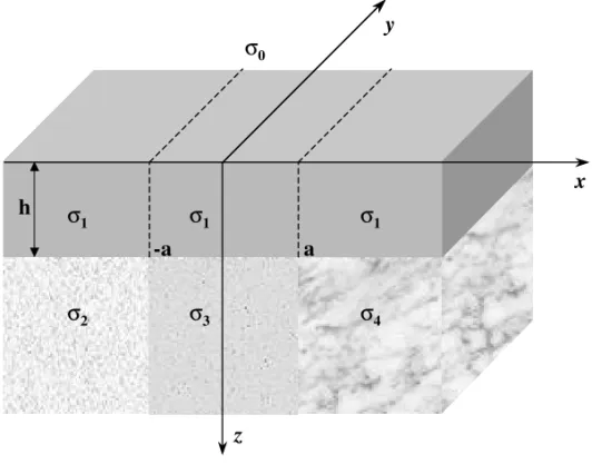
Let a TE mode EM plane wave, which propagates in the positivezdirection, be scattered by a geological structure consisting of a buried vertical dike as depicted in Figure 1. The horizontal layer thickness ish, its electrical conductivity isσ1, and it is in contact along the planez=0 with an infinitely resistive half-space (z < 0). The vertical dike presents an electrical conductivityσ3
layer is in contact with both the dike and the two quarter-spaces along the horizontal planez= +h.
σ 4 σ
3 σ
2 σ
1 σ1 σ1
x y
z
a -a
h
σ 0
Fig. 1 – Representation of the physical and geometrical properties of the buried vertical dike model.
For the TE mode the electric vector is always along they direction, and for the described model the total electrical conductivity presents a constant and finite value in each medium. So the problem consists in finding the solution for the two-dimensional homogeneous Helmholtz wave equation in each medium:
∂2En ∂x2 +
∂2En ∂z2 +k
2
nEn=0 n=0,1,2,3,4, (1)
where:
• kn =
√
−iωµ0(σn+iωε0), is the propagation constant in each medium; ω is the angular
frequency;µ0 andε0 are the free-space values of, respectively, the magnetic permeability and the dielectric permittivity; andσnis the conductivity.
• Enrepresents they component of the electric field vector.
En =Ey(x, z, ω)=
∞
−∞
ey(x, z, t )e−iωtdt .
Representation of the Fields
1. For−∞< z <0:
E0,2 = EI+E0R,2+
∞
0
f0,2eu0xcos(αz)+g0,2eu0zcos(αx)
dα; (2)
E0,3 = EI+E0R,3+
∞
0
(f0,3Ae−u0x+f0,3Beu0x)cos(αz)+g0,3eu0zcos(αx)
dα; (3)
E0,4 = EI+E0R,4+
∞
0
f0,4e−u0xcos(αz)+g0,4eu0zcos(αx)
dα. (4)
2. For 0< z < h:
E1,2 = E0T,2+E R 1,2+
∞
0
f1,2eu1xcos(αz)+(g1,2Ae−u1z+g1,2Beu1z)cos(αx)
dα; (5)
E1,3 = E0T,3+E R 1,3+
∞
0
(f1,3Ae−u1x+f1,3Beu1x)cos(αz)+
(g1,3Ae−u1z+g1,3Beu1z)cos(αx)
dα; (6)
E1,4 = E0T,4+E R 1,4+
∞
0
f1,4e−u1xcos(αz)+(g1,4Ae−u1z+g1,4Beu1z)cos(αx)
dα. (7)
3. Forh < z <∞:
E2 = E2T +
∞
0
f2eu2xcos(αz)+g2e−u2zcos(αx)dα; (8)
E3 = E3T +
∞
0
(f3Ae−u3x+f3Beu3x)cos(αz)+g3e−u3zcos(αx)
dα; (9)
E4 = E4T +
∞
0
f4e−u4xcos(αz)+g4e−u4zcos(αx)dα. (10)
Where: EI
= e−ik0z represents the incident field forz < 0;ER
0,j = R0,je ik0z,R0
,j are the
free-space reflection coefficients; E0T,j = T0,je−ik1z, T0,j are the transmission coefficients from
the free-space into the horizontal layer; ER
1,j = R1,jeik1(z−h), R1,j are the reflection coefficients
for the horizontal layer relative to medium 2, 3 and 4 respectively; EjT = T1,je−ikj(z−h),T1,j are
the transmission coefficients from the horizontal layer into medium 2, 3 e 4 respectively; and
un =
α2−k2
n, represents the wave number in the transformed space.
Boundary Conditions
To solve the problem it is necessary to find the 24 spectral components,f0,2,g0,2,f0,3A,f0,3B,g0,3, f0,4,g0,4,f1,2,g1,2A,g1,2B,f1,3A,f1,3B,g1,3A,g1,3B,f1,4,g1,4A,g1,4B,f2,g2,f3A,f3B,g3,f4, and g4, employing the pertinent boundary conditions.
li lim x→λ
∂Ei,j
∂x = lmxlim→λ
∂Em,j+1
∂x and Ei,j = Em,j+1, in thexdirection;
li lim z→γ
∂Ei,j
∂z = lmzlim→γ
∂Em,j+1
x
= −
a
x
=
a
z
=
0
z
=
h
k
0,
E
0,2k
0,
E
0,3k
0,
E
0,4✲
x
❄
z
k
1,
E
1,2k
1,
E
1,3k
1,
E
1,4k
2,
E
2k
3,
E
3k
4,
E
4h
✻
❄
✲
H
x❄
H
z✠
E
yFig. 2 – Representation of the incident field components and of the electric field in each medium.
The weighing factorlnis the inverse of impedance per unit length in each medium;λ= ±a; and γ =0 orh.
Substituting Equations (2)–(10) in the boundary conditions and putting in the left hand side only the terms that are function either of cos(αx)or of cos(αz), we obtain the following system of twenty four integral equations in twenty four unknowns – the spectral components:
∞
0 u0
e−u0af0
,2+eu0af0,3A−e−u0af0,3B
cos(αz)dα
=
∞
0
−eu0zg0
,2+eu0zg0,3
αsin(αa)dα (11)
∞
0
e−u0af0
,2−eu0af0,3A−e−u0af0,3B
cos(αz)dα
=
∞
0
−eu0zg0
,2+eu0zg0,3
cos(αa)dα+e−ik0z(E3−E2)+eik0z(R0
,3−R0,2) (12)
∞
0 u0
−e−u0af0
,3A+eu0af0,3B+e−u0af0,4
cos(αz)dα
=
∞
0
eu0zg0
,3−eu0zg0,4
∞
0
e−u0af0
,3A+eu0af0,3B−e−u0af0,4
cos(αz)dα
=
∞
0
−eu0zg0
,3+eu0zg0,4
cos(αa)dα+e−ik0z(E4−E3)
+ eik0z(R0
,4−R0,3) (14)
∞
0
u1e−u1af1
,2+eu1af1,3A−e−u1af1,3B
cos(αz)dα
=
∞
0
−e−u1zg1
,2A−eu1zg1,2B+e−u1zg1,3A+eu1zg1,3B
αsin(αa)dα (15)
∞
0
e−u1af1
,2−eu1af1,3A−e−u1af1,3B
cos(αz)dα
=
∞
0
−e−u1zg1
,2A−eu1zg1,2B+e−u1zg1,3A+eu1zg1,3B
cos(αa)dα
+ eik1z(T0
,3−T0,2)+e−ik1(z−h)(R1,3−R1,2) (16)
∞
0 u1
−e−u1af1
,3A+eu1af1,3B+e−u1af1,4
cos(αz)dα
=
∞
0
e−u1zg1
,3A+eu1zg1,3B−e−u1zg1,4A−eu1zg1,4B
αsin(αa)dα (17)
∞
0
e−u1af1
,3A+eu1af1,3B−e−u1af1,4
cos(αz)dα
=
∞
0
−e−u1zg1
,3A−eu1zg1,3B+e−u1zg1,4A+eu1zg1,4B
cos(αa)dα
+ e−ik1z(T0
,4−T0,3)+eik1(z−h)(R1,4−R1,3) (18)
∞
0
l2u2e−u2af2
+l3u3eu3af3
A−l3u3e−u3af3B
cos(αz)dα
=
∞
0
−l2e−u2zg2+l3e−u3zg3αsin(αa)dα (19)
∞
0
e−u2af2
−eu3af3
A−e−u3af3B
cos(αz)dα
=
∞
0
−e−u2zg2+e−u3zg3cos(αa)dα−e−ik2(z−h)T1
∞
0
−l3u3e−u3af3
A+l3u3eu3af3B+l4u4e−u4af4
cos(αz)dα
=
∞
0
l3e−u3zg3−l4e−u4zg4αsin(αa)dα (21)
∞
0
e−u3af3
A+eu3af3B−e−u4af4
cos(αz)dα
=
∞
0
−e−u3zg3+e−u4zg4cos(αa)dα−e−ik3(z−h)T1
,3+e−ik4(z−h)T1,4 (22)
∞
0
l0u0g0,2+l1u1g1,2A−l1u1g1,2B
cos(αx)dα
=il0k0(EI −R0,2)−il1k1(T0,2−e−ik1h)R1,2) (23)
∞
0
g0,2−g1,2A−g1,2B
cos(αx)dα
=
∞
0
−eu0xf0
,2+eu1xf1,2
dα−EI−R0,2+T0,2+e−ik1hR1,2 (24)
∞
0
−l1u1e−u1hg1
,2A+l1u1eu1hg1,2B+l2u2e−u2hg2
cos(αx)dα
=
∞
0
l1eu1xf1
,2+l2eu2xf2
αsin(αh)dα
− il1k1(e−ik1hT0
,2−R1,2)+il2k2T1,2 (25)
∞
0
e−u1hg1
,2A+eu1hg1,2B−e−u2hg2
cos(αx)dα
=
∞
0
−eu1xf1
,2−eu2xf2
cos(αh)dα−eik1hT0
,2−R1,2+T1,2 (26)
∞
0
l0u0g0,3+l1u1g1,3A−l1u1g1,3B
cos(αx)dα
=il0k0(EI −R0,3)−il1k1(T0,3−e−ik1hR1,3) (27)
∞
0
g0,3−g1,3A−g1,3B
cos(αx)dα
=
∞
0
−e−u0xf0
,3A−eu0xf0,3B+e−u1xf1,3A+eu1xf1,3B
− EI−R0,3+T0,3+e−ik1hR1,3 (28)
∞
0
−l1u1e−u1hg1
,3A+l1u1eu1hg1,3B+l3u3e−u3hg3
cos(αx)dα
=
∞
0
l1e−u1xf1
,3A+l1eu1xf1,3B−l3e−u3xf3A−l3eu3xf3B
αsin(αh)dα
+ il1k1(T0,3−e−ik1hR1,3)+il3k3eik3hT1,3 (29)
∞
0
e−u1hg1
,3A+eu1hg1,3B−e−u3hg3
cos(αx)dα
=
∞
0
−e−u1xf1
,3A−eu1xf1,3B+e−u3xf3A+eu3xf3B
cos(αh)dα
− e−ik1hT0
,3−R1,3+T1,3 (30)
∞
0
l0u0g0,4+l1u1g1,4A−l1u1g1,4B
cos(αx)dα
=il0k0(EI −R0,4)−il1k1(T0,4−e−ik1hR1,4) (31)
∞
0
g0,4−g1,4A−g1,4B
cos(αx)dα
=
∞
0
−e−u0xf0
,4+e−u1xf1,4
dα−EI −R0,4+T0,4+e−ik1hR1,4 (32)
∞
0
−l1u1e−u1hg1
,4A+l1u1eu1hg1,4B+l4u4e−u4hg4
cos(αx)dα
=
∞
0
l1e−u1xf1
,4−l4e−u4xf4
αsin(αh)dα+il1k1(T0,4−e−ik1hR1,4)
+ il4k4eik4hT1
,4 (33)
∞
0
e−u1hg1
,4A+eu1hg1,4B−e−u4hg4
cos(αx)dα
=
∞
0
[−e−u1xf1
,4+e−u4xf4]cos(αh)dα−e−ik1hT0,4−R1,4+T1,4. (34)
It will prove to be useful to organize this system in a matrix form. Therefore, Equations (11)–(34) can be rewritten in the following form:
∞
0
W(α)·φ (α)cos(αβ)dα=
∞
0
M(α;β)·φ (α)dα+Y(β). (35)
pentadiagonal square matrix (24×24), which contains the constant coefficients constituted by six sparse submatrixes,
W(β)=
(W0 1)4×4
(W11)4×4 0
(W2)4×4
(W23)4×4
0 (W33)4×4 (W4
3)4×4
24×24
:
W1j =
uje−uja uje−uja −uje−uja 0 e−uja −e−uja −e−uja 0
0 −ujeuja ujeuja uje−uja
0 e−uja euja −e−uja
, j =0,1,
W2 =
l2u2e−u2a l3u3eu3a −l3u3e−u3a 0
e−u2a −eu3a −e−u3a 0 0 −l3u3e−u3a l3u3e−u3a l4u4e−u4a 0 e−u3a eu3a −e−u4a
,
Wi3 =
l0u0 l1u1 −l1u1 0
1 1 1 0
0 −l1u1e−u1h l1u1eu1h l
iuie−uih
0 e−u1h eu1h −e−uih
, i=2,3,4,
M(α;β)is a sparse square matrix (24×24), formed by six sparse submatrixes,
M(α;β)=
0 (M0)4×9 0
0 (M1)4×10
0 (M2)4×9
(M3)4×9 0
(M4)4×10 0
0 (M5)4×9 0
24×24
:
M0=
−eu0zSa 0 0 0 eu0zSa 0 0 0 0
−eu0zCa 0 0 0 eu0zCa 0 0 0 0
0 0 0 0 eu0zSa 0 0 0 −eu0zSa 0 0 0 0 −eu0zCa 0 0 0 −eu0zCa
M1=
−e−u1zSa −eu1zSa 0 0 e−u1zSa eu1zSa 0 0 0 0
−e−u1zCa −eu1zCa 0 0 e−u1zCa eu1zCa 0 0 0 0 0 0 0 0 e−u1zSa eu1zSa 0 0 −e−u1zSa −eu1zSa 0 0 0 0 −e−u1zCa −eu1zCa 0 0 e−u1zCa eu1zCa
,
M2=
−l2e−u2zSa 0 0 0 l3e−u3zSa 0 0 0 0
−e−u2zCa 0 0 0 e−u3zCa 0 0 0 0
0 0 0 0 l3e−u3zSa 0 0 0 −l4e−u4zSa 0 0 0 0 −e−u3zCa 0 0 0 e−u4zCa
,
M3=
S0 0 0 0 −S0 0 0 0 0
−eu0xC0 0 0 0 eu1xC0 0 0 0 0
0 0 0 0 l1eu1xSh 0 0 0 −l2eu2xSh 0 0 0 0 −eu1xCh 0 0 0 eu2xCh
,
M4=
S0 S0 0 0 S0 −S10 0 0 0 0
−e−u0xC0 −eu0xC0 0 0 e−u1xC0 eu1xC0 0 0 0 0 0 0 0 0 l1e−u1xSh l1eu1xSh 0 0 −l3e−u3xSh −l3eu3xSh
0 0 0 0 −e−u1xCh −eu1xCh 0 0 e−u3xCh eu3xCh
,
M5=
−S0 0 0 0 S0 0 0 0 0
−S0 0 0 0 S0 0 0 0 0
−e−u0xC0 0 0 0 e−u1xC0 0 0 0 0
0 0 0 0 l1e−u1xSh 0 0 0 −l4e−u4xSh 0 0 0 0 −e−u1xCh 0 0 0 e−u4xCh
.
φ =
f0,2 f0,3A f0,3B f0,4 f1,2 f1,3A f1,3B f1,4
f2 f3A f3B f4 g0,2 g0,3 g0,4 g1,2A g1,2B g1,3A g1,3B g1,4A g1,4B g2 g3 g4
; Y(β)=
0
−e−ik0z(EI
0,2−E0I,3)−eik0z(R0,2−R0,3)
0
−e−ik0z(EI
0,3−E0I,4)−eik0z(R0,3−R0,4)
0
−e−ik1z(T0
,2−T0,3)−eik1(z−h)(R1,2−R1,3)
0
−e−ik1z(T0
,3−T0,4)−eik1(z−h)(R1,3−R1,4)
0
−e−ik2(z−h)T1
,2+e−ik3(z−h)T1,3
0
−e−ik3(z−h)T1
,3+e−ik4(z−h)T1,4 il0k0(E0I,2−R0,2)−il1k1(T0,2−e−ik1hR1,2)
−E0I,2−R0,2+T0,2+e−ik1hR1,2 il1k1(T0,2−e−ik1hR1,2)−il2k2T1,2
−e−ik1hT0
,2−R1,2+T1,2
il0k0(E0I,3−R0,3)−il1k1(T0,3−e−ik1hR1,3)
−EI
0,3−R0,3+T0,3+e−ik1hR1,3 il1k1(T0,3−e−ik1hR1,3)−il3k3T1,3
−e−ik1hT0
,3−R1,3+T1,3
il0k0(E0I,4−R0,4)−il1k1(T0,4−e−ik1hR1,4)
−E0I,4−R0,4+T0,4+e−ik1hR1,4 il1k1(T0,4−e−ik1hR1,4)−il3k3T1,4
−e−ik1hT0
,4−R1,4+T1,4
.
Determination of the Spectral Components
Applying the inverse cosine Fourier transformF−1
c (β −→α)in Equation (35), we obtain:
• Left Hand Side,
Fc−1
∞
0
W(α)·φ (α)cos(αβ)dα
= W(α)·φ (α); (36)
• Right Hand Side,
F−1 c
∞
0
M(α;β)·φ (α)dα+Y(β) = 2 π ∞ 0 ¯
M(α;ξ )·φ (ξ )dξ +y(α)
Where:
¯
M =
0 (M¯a
0)4×9 0
0 (M¯ a1)4×10
0 (M¯a2)4×9 (M¯h
3)4×9 0
(M¯ h4)4×10 0
0 (M¯h
5)4×9 0
24×24
:
¯
M0 =
Sa
0 0 0 0 −S0a 0 0 0 0
C0a 0 0 0 −C0a 0 0 0 0 0 0 0 0 −S0a 0 0 0 S0a
0 0 0 0 Ca
0 0 0 0 −C0a
,
¯
M1 =
−S1a S1a 0 0 S1a −S1a 0 0 0 0
−Ca
1 C1a 0 0 C1a −C1a 0 0 0 0
0 0 0 0 S1a −S1a 0 0 −S1a S1a
0 0 0 0 −C1a C1a 0 0 C1a −C1a
,
¯
M2 =
−l2S2a 0 0 0 l3S3a 0 0 0 0
−Ca
2 0 0 0 C3a 0 0 0 0
0 0 0 0 l3S3a 0 0 0 −l4S4a
0 0 0 0 −C3a 0 0 0 C4a
,
¯
M3 =
S00 0 0 0 −S00 0 0 0 0
C00 0 0 0 −C10 0 0 0 0 0 0 0 0 l1Sh
1 0 0 0 l2S2h
0 0 0 0 C1h 0 0 0 −C2h
,
¯
M4 =
−S0
0 S00 0 0 S10 −S10 0 0 0 0
−C00 C00 0 0 C10 −C10 0 0 0 0
0 0 0 0 l1S1h −l1S1h 0 0 −l3S3h l3S3h
0 0 0 0 −Ch
1 C1h 0 0 C3h −C3h
,
¯
M5 =
−S00 0 0 0 S10 0 0 0 0
−C0
0 0 0 0 C00 0 0 0 0
0 0 0 0 l1S1h 0 0 0 −l4S4h
0 0 0 0 −C1h 0 0 0 C4h
.
• Snj = ∓ un(ξ ) u2
n(ξ )+α2
ξsin(ξj );
• Cnj = ∓ un(ξ ) u2
n(ξ )+α2
cos(ξj ).
Forj =a,hor 0 andn=1, 2, 3 and 4.
y(α)=
0
2ik0
π(α2−k2 0)
(R0,2−R0,3)
0
2ik0
π(α2−k2 0)
(R0,3−R0,4)
0
− 2ik1
π(α2−k2 1)[
(T0,2−T0,3)−(R1,2−R1,3)e−ik1h]
0
− 2ik1
π(α2−k2 1)[
(T0,3−T0,4)−(R1,3−R1,4)e−ik1h]
0
−2ik2eik2h
π(α2−k2 2)
T1,2+ 2ik3e
ik3h π(α2−k2 3)
T1,3
0
−2ik3eik3h
π(α2−k2 4)
T1,3+ 2ik4e
ik4h π(α2−k2
4)
T1,4
0 0 0 0 0 0 0 0 0 0 0 0 .
From Equations (36) and (37) we obtain,
W(α)·φ (α)=y(α)+
∞
0
¯
M(α;ξ )φ (ξ )dξ (38)
Multiplying Equation (38) byW−1(α), we obtain,
φ (α)=ψ (α)+
∞
0
Notice that W−1(α) represents the inverse matrix, obtained by a straightforward operation; ψ (α) = W−1(α)
·y(α) represents the vector of the independent constants; and K(α;ξ ) =
W−1(α)
· ¯M(α;ξ )is a sparse square matrix, denominated nucleus matrix.
The integral equations of the system (39) are classified as Fredholm singular integral equations of the second kind. The regular part,0∞K(α;ξ )φ (ξ )dξis a Riemann improper integral, possessing a finite value. So, the solution of the equation (39) can be obtained employing the method of successive approximations (Kondo 1991):
φn(α) = n
m=0
φm(α)= ψ (α)+( o
K1(α;ξ )+
o
K2(α;ξ )+. . .
+
o
Kn−1(α;ξ ))◦ψ (α)+
o
Kn(α;ξ )◦ψ (α),
(40)
because
φ0(α)=φ0(α)=ψ (α), (41)
and
φ1(α)=
∞
0
K(α;ξ0)φ0(ξ0)dξ0, (42)
φm(α)=
∞
0
K(α;ξm−1)dξm−1. . .
∞
0
K(α;ξ0)φ0(ξ0)dξ0. (43)
Where:
o
Kn(α
;ξ ) =
o
K1(α
;ξ ) ◦
o
Kn−1(α
;ξ ), forn >1, and
o
K1(α
;ξ ) = K(α;ξ ).
The elements of the vectorφn(α) are the spectral components used to calculate the scattered
electric field in the nine domains of the model under study. It is sufficient the series (40) be convergent in order for
lim
n→∞φn(α)=θ (α). (44) A necessary but not sufficient condition for the convergence of the series is that limm→∞φm(α) = 0. (Sampaio and Fokkema 1992) verified numerically that the terms of the
series decrease and the series remains bounded for up to five terms for the model of a vertical fault, and we expect the model of the buried dike to present a similar behavior. However the rigorous proof of the convergence of the series is a difficult mathematical problem and we lack such a proof.
NUMERICAL RESULTS
Basic Concepts
than the modulus of the constant of propagation of the air. In the present case this implies that
|kn| ≫ |k0|, forn= 1, 2, 3, 4. Therefore the reflection and transmission coefficients assume the
following values:
R0,j = rj−1 rj+1;
R1,j = sj −1 rj +1
tj;
T0,j = sj+1 rj+1
tj; T1,j =
2sj rj +1
tj;
rj =
k0[k1+kjtgh(ik1h)] k1[kj +k1tgh(ik1h)];
sj = k1 kj
;
tj =
2rj
sj(1+e−ik1h)+(1−e−ik1h)
;
wherehis the overburden thickness.
Computation of the Spectral Components
Due to the fast convergence of the terms of the series, we will compute only the first term of the series (zero-order term), employing Equation (41). With the simplification of the series the original system reduces to a sparse system of 12 linear equations in 12 unknowns.
W(α)·φ (α)=y(α). (45)
The solution of the system of equations (45) is relatively simple, because its matrix is sparse, pentadiagonal, and contains only three 4×4 independent submatrixes.
Graphical Representation of the Spectral Components
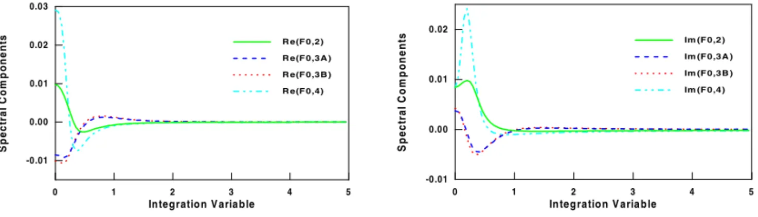
The convergence of the spectral components can be verified through a graphical analysis from the behaviour of each element of the vector φ as a function of the integration variable α. In order to do that we applied the zero-order solution to the following model of the earth: a vertical dike of width 2a = 0.5|k3| and conductivityσ3 = 0.1 S/m, immersed between two quarter-spaces of conductivities σ2 = 0.01 S/m andσ4 = 0.005S/m, and covered by a horizontal layer of conductivityσ1=0.05S/mand thicknessh=0.01|k3|.
Figure (3) displays the variation of the real and the imaginary parts of the spectral components on the surface of the earth. They are the kernels of the equations that represent the electric field on the top of the overburden.
0 1 2 3 4 5
In teg ratio n V aria b le
-0.01 0.00 0.01 0.02 0.03
S
p
ect
ral
C
o
m
p
o
n
e
n
ts R e(F 0,2)
R e(F 0,3A ) R e(F 0,3B ) R e(F 0,4)
0 1 2 3 4 5
In teg ratio n V aria b le
-0.01 0.00 0.01 0.02
S
p
ect
ral
C
o
m
p
o
n
e
n
ts Im (F 0,2)
Im (F 0,3A ) Im (F 0,3B ) Im (F 0,4)
Fig. 3 – Variation of the real and the imaginary parts of the spectral components as a function of the normalized integration variable.
Computation and Representation of the Normalized Electric Field
After the determination of the spectral components and the check of the convergence of the integrals we computed the normalized electric field, E |k3|
H0ωµ0, at the surface of the earth for the proposed dike model, employing Equations (5), (6) and (7). We employed different geoelectric parameters to simulate distinct models.
Figure (4) displays the variation of the real and the imaginary parts of the normalized electric field onz = 0 as a function of|k3|x, for the vertical dike model with the following parameters: variable dike width 2a and overburden thicknessh;σ1=0.05S/m;σ2 =σ4 =0.005S/m; and
σ3=0.1S/m. The electric field has been computed for the following values ofp1=2a/ h: 1; 5; 10; 50; and 200.
-3.0 -2.0 -1.0 0.0 1.0 2.0 3.0
W ave N u m b er
-4.5 -4.0 -3.5 -3.0 -2.5 -2.0 -1.5 -1.0 -0.5
N
o
rm
al
iz
ed
E
le
ct
ri
c
F
iel
d
p 1 = 1 ,0 p 1 = 5 ,0 p 1 = 1 0 ,0 p 1 = 5 0 ,0 p 1 = 2 0 0 ,0
-3.0 -2.0 -1.0 0.0 1.0 2.0 3.0
W ave N u m b er
-5.0 -4.0 -3.0 -2.0 -1.0 0.0 1.0 2.0 3.0
N
o
rm
al
iz
ed
E
le
ct
ri
c
F
iel
d
p 1 = 1 ,0 p 1 = 5 ,0 p 1 = 1 0 ,0 p 1 = 5 0 ,0 p 1 = 2 0 0 ,0
Fig. 4 – Variation of the real and the imaginary parts of the scattered electric field as a function of the wave number |k3|x, onz=0, where:σ1=0.05S/m;σ2=σ4=0.005S/m;σ3=0.1S/m; and given values ofp1= 2ha.
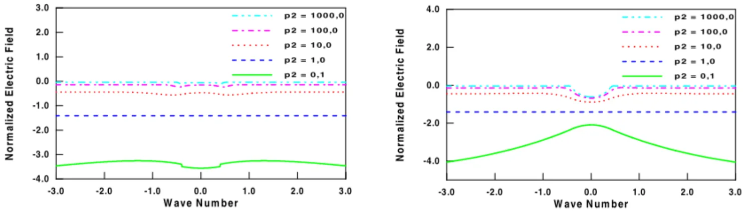
field on z = 0 as a function of|k3|x, for the vertical dike model with the following parameters: variable conductivity of the surrounding rocks and the dike;σ1=0.05S/m; overburden thickness such thath= 0.02|k3|; and width of the dike such that 2a = 0.4|k3|. The electric field has been computed for the following values ofp2=σ3/σ2: 0.1; 1; 10; 100; and 1000.
-3.0 -2.0 -1.0 0.0 1.0 2.0 3.0
W ave N u m b er
-4.0 -3.0 -2.0 -1.0 0.0 1.0 2.0 3.0
N
o
rm
al
iz
ed
E
le
ct
ri
c
F
iel
d
p 2 = 1 0 0 0 ,0 p 2 = 1 0 0 ,0 p 2 = 1 0 ,0 p 2 = 1 ,0 p 2 = 0 ,1
-3.0 -2.0 -1.0 0.0 1.0 2.0 3.0
W ave N u m b er
-4.0 -2.0 0.0 2.0 4.0
N
o
rm
al
iz
ed
E
le
ct
ri
c
F
iel
d
p 2 = 1 0 0 0 ,0 p 2 = 1 0 0 ,0 p 2 = 1 0 ,0 p 2 = 1 ,0 p 2 = 0 ,1
Fig. 5 – Variation of the real and the imaginary parts of the scattered electric field onz=0 as a function of the wave number|k3|x, where: σ1=0.05S/m;h=0.02|k3|; 2a=0.4|k3|; and given values ofp2= σσ32.
We observe in Figure (5) that, as expected, the behaviour of the curves for p2 = 0.1 is the opposite to the curves forp2>1. The real part curves forp2>1 reach a maximum value atx=0 and have an inflection point at|x| =a. Forp2=0.1 these curves reach a minimum atx=0 and they also have an inflection point at|x| =a. The behaviour of the imaginary curves is exactly the opposed.
Figure (6) displays the variation of the real and the imaginary parts of the normalized electric field on z = 0 as a function of|k3|x, for the vertical dike model with the following parameters: variable conductivity of the overburden and the dike; overburden thickness such thath=0.02|k3|; dike width such that 2a = 0.4|k3|; and σ2 = σ4 = 0.0005 S/m. The electric field has been computed for the following values ofp3=σ3/σ1: 0.1; 0.4; 1; 10; and 100.
-3.0 -2.0 -1.0 0.0 1.0 2.0 3.0
W ave N u m b er
-5.0 -4.0 -3.0 -2.0 -1.0
N
o
rm
al
iz
ed
E
le
ct
ri
c
F
iel
d
p 3 = 0 ,1 p 3 = 1 ,0 p 3 = 1 0 ,0 p 3 = 1 0 0 ,0 p 3 = 1 0 0 0 ,0
-3.0 -2.0 -1.0 0.0 1.0 2.0 3.0
W ave N u m b er
-5.0 -4.0 -3.0 -2.0 -1.0 0.0 1.0 2.0 3.0
N
o
rm
al
iz
ed
E
le
ct
ri
c
F
iel
d
p 3 = 0 ,1 p 3 = 1 ,0 p 3 = 1 0 ,0 p 3 = 1 0 0 ,0 p 3 = 1 0 0 0 ,0
Fig. 6 – Variation of the real and the imaginary parts of the scattered electric field onz=0 as a function of the wave number|k3|x, where: σ2=σ4=0.0005S/m; 2a=0.4|k3|;h=0.02|k3|; and given values ofp3= σσ31.
However this distinction does not happen in the imaginary part curves. For them the contacts are always well defined. The maximum value is observed atx =0 forp3≥1, whereas forp3<0.1 the position of the maximum is not well defined.
CONCLUSION
The complete and exact algebraic solution of the scattering of a monochromatic EM plane wave, for the case of a vertical dike immersed in two quarter-spaces and overlaid by a horizontal layer, was determined. As a first step, zero-order terms of the series representation of the spectral components were selected to compute an approximate value of the electric field above the vertical dike.
The results of the modeling show that: 1) for the outcropping dike, h → 0, the contacts between the dike and the surrounding rocks are very well defined; 2) for a large thickness of the overburden,h→ ∞, the contacts between the dike and the quarter-spaces are not defined; 3) when the conductivity of the overburden is much larger than the conductivity of the dike,σ1 >> σ3, it is not possible to define the contacts between the dike and the surrounding rocks employing the real component of the electric field, but the contacts are defined through the imaginary component. The results show the precision of the zero-order terms in the calculation of the secondary electric field. So they can be used in the computation to substitute other techniques with advantage. Therefore the expressions of the analytical solution of the electric field are fundamental for the interpretation of magnetotelluric, or VLF (Very Low Frequency) data, associated to the geophysical exploration.
ACKNOWLEDGMENTS
We acknowledge our fellowships and the grant from CNPq (Brazilian National Science Foundation). We thank the fruitful comments from Prof. M. Popov. We also thank the help from Mr. J. Lago in the preparation of the manuscript.
RESUMO
Estabelecemos a solução exata e completa do espalhamento de uma onda plana eletromagnética no domínio
da freqüência e no modo elétrico transverso por um dique vertical soterrado por uma camada condutora. Uma representação integral composta de transformadas unilaterais de Fourier descreve os componentes do campo elétrico espalhado em cada um dos cinco meios: ar, cobertura, dique e as rochas encaixantes
de cada lado do dique. A determinação dos termos da série que representa os componentes espectrais das integrais de Fourier requer a inversão numérica de uma matriz esparsa e o método das aproximações
sucessivas. Calculamos o termo de ordem zero da série para os componentes espectrais da camada de cobertura, para valores especificados dos parâmetros geométricos e elétricos do modelo. Este resultado permitiu determinar um valor aproximado da variação do campo elétrico no contato entre o ar e a camada
Palavras-chave: espalhamento, onda eletromagnética, dique vertical.
REFERENCES
Avdeev DB, Kuvshinov AV, Pankratov OV and Newman GA. 1997. High-performance three-dimensional electromagnetic modelling using modified Neumann series. Wide-band numerical solution and examples. J Geomagn Geoeletr 49: 1519-1539.
Batista LS and Sampaio EES.1999. Scattering of Electromagnetic Plane Waves by a Buried Vertical Dike. In: 6t hInternational Congress of the Sociedade Brasileira de Geofísica, Rio de Janeiro. Expanded Abstracts in CD-ROM, Rio de Janeiro.
Cagniard L.1953. Basic Theory of the Magneto-Telluric Method of Geophysical Prospecting. Geophysics
18: 605-635.
Gupta PK, Bennett LA and Raiche AP.1987. Hybrid calculations of the three-dimensional electro-magnetic response of buried conductors. Geophysics 52: 301-306.
Kondo J.1991. Integral Equations. Oxford applied mathematics and computing science series. Oxford:
Oxford University Press, 440 p.
Livelybrooks D.1993. Program 3D FEEM: a multidimensional electromagnetic finite element model. Geophys J Int 114: 443-458.
Sampaio EES and Fokkema JT.1992. Scattering of Monochromatic Acoustic and Electromagnetic Plane
Waves By Two Quarter Spaces. J Geoph Res 97: 1953-1963.
Sampaio EES and Popov MM.1997. Zero-Order Time Domain Scattering of Electromagnetic Plane Waves by Two Quarter Spaces. Radio Science 32: 305-315.
Sommerfeld A.1896. Mathematical Theory of Diffraction. Math Ann 47: 317-374.
Tikhonov AN. 1950. Determination of the Electrical Characteristics of the Deep Strata of the Earth’s
Crust. Doklady 73: 295-297.
Wiener N and Hopf E.1931. One Class of Singular Integrals. Proc Prussian Acad Math Phys Sec 696-796.