Transverse Vibrations in Beams Supported by a Piece-Wise Homogeneous Visco-Elastic Foundation

Abstract

Transversal vibrations induced by a load moving uniformly along an infinite beam resting on a piece-wise homogeneous visco-elastic foundation are studied. Special attention is paid to the additional vibrations, conventionally referred to as transition radiations, which arise as the point load traverses the place of foundation discontinuity. The governing equations of the problem are solved by the normal-mode analysis. The solution is expressed in a form of infinite sum of orthogonal natural modes multiplied by the generalized coordinate of displacement. The natural frequencies are obtained numerically exploiting the concept of the global dynamic stiffness matrix. This ensures that the frequencies obtained are exact. The methodology has restrictions neither on velocity nor on damping. The approach looks simple, though, the numerical expression of the results is not straightforward. A general procedure for numerical implementation is presented and verified. To illustrate the utility of the methodology parametric optimization is presented and influence of the load mass is studied. The results obtained have direct application in analysis of railway track vibrations induced by high-speed trains when passing regions with significantly different foundation stiffness.

Keywords: moving load, moving mass, transversal vibration, transition radiation,

normal-mode analysis, dynamic stiffness matrix, natural frequencies, orthonormal mode shapes.

1 Introduction

The rapid growth of high-speed railway network and the considerable evolution of train vehicles capable to operate at more than 500 km/h, gave raise to a number of related problems that have motivated a significant amount of scientific work. The amplification of train-induced vibrations, caused by inhomogeneities in the track foundation, certainly belongs to the issues still demanding further attention.

Transverse Vibrations in Beams Supported by a

Piece-Wise Homogeneous Visco-Elastic Foundation

Z. Dimitrovová1and L. Frýba2

1_{UNIC, Department of Civil Engineering}

New University of Lisbon, Portugal

2Institute of Theoretical and Applied Mechanics

Academy of Sciences of the Czech Republic, Prague, Czech Republic

in B.H.V. Topping, L.F. Cost a Neves, R.C. Barros, ( Edit ors) , " Proceedings of t he Tw elft h I nt ernat ional Conference on Civil, St ruct ural and Environm ent al

Theoretical basis of this occurrence lies in the fact, that when the load passes the place of discontinuity in the supporting structure, additional vibrations, conventionally referred to as transition radiations, are generated. Radiation waves travel backward and forward from the place of discontinuity and may significantly amplify the original waves. As a consequence, the track deterioration is aggravated and concerns related to the vehicle stability and passengers comfort must be taken into account.

The inhomogeneities in the foundation stiffness have origin in geotechnical conditions, in the state of degradation of the track or in an alteration of the structural design. The representative values can differ by orders and their change can be quite sharp. The above mentioned cases refer for instance to situations, where the track settlement due to non-elastic deformations in the ballast and subground is so high, that the full contact between some sleepers and the ballast bed is lost. Then “hanging” sleepers appear and this induces an irregularity of the track stiffness. Other situations cover an embankment-to-bridge or tunnel transition; switch from ballasted to slab track, regions where the high-speed line crosses underground structures, and so on.

An insight into a problem of induced vibrations can be acquired from simplified models, which have a closed form solution. Such approach has many advantages: (i) only main results are available, so they are simple to analyse; (ii) the results preserve parameters dependence allowing for direct sensitivity analysis; (iii) numerical evaluation can be carried out only in places of interest. Due to the simplifying assumptions, however, the results obtained correspond only to the estimate of the real structure response to a moving load.

In this paper, the transient dynamic response of a one-dimensional piece-wise homogeneous structure subjected to uniformly moving time dependent transverse load is expressed in an analytical form exploiting the normal-mode analysis. The structure is assumed in the form of an infinite beam resting on a visco-elastic foundation. The methodology has restrictions neither on velocity magnitude nor on material or mass damping coefficients. Discontinuities in the foundation stiffness parameter, in the flexural rigidity of the beam, in the mass per unit length or in the damping coefficient can be implemented. It is assumed that there is only finite number of discontinuities. Special attention is paid to the transition radiation. The transient shapes of the beam are presented in order to visualize the radiation process.

The concept of the global dynamic stiffness matrix [5] of the structure is used to determine natural frequencies and normal modes. This ensures that the natural frequencies are exact. With this purpose structural elements _{are defined as the}

longest possible parts of the structure, where all properties are homogeneous. This is probably the most accurate way to deal with the dynamic behaviour of a distributed-parameter beam. Nevertheless, this methodology is not widely used. The reason is the numerical difficulty in evaluation of higher frequencies. Author’s previous work [6] focused on avoiding the natural frequencies evaluation and suggested different methodology. Transition radiation was calculated by linking together analytical solutions of each structural element by continuity conditions. In this paper a general procedure for numerical implementation according to the normal-mode analysis is presented and verified. Procedures are programmed in MAPLE [7] and MATLAB [8] environment. To illustrate the utility of the methodology parametric optimization is presented and the influence of the load mass is studied.

The paper is organized in the following way. In Section 2 the motivation for the methodology adopted is given, governing equations are presented and simplifying assumptions are stated. For the sake of simplicity Euler-Bernoulli formulation is presented only. In Section 3 the closed form solution is given and the concept of the global dynamic stiffness matrix is explained. Also the rules for the numerical expression of the results are established and the methodology for extension to infinite beams is presented. Section 4 shows case studies and in Section 5 summary of the achievements and further challenges are stated. Results and conclusions have direct application on knowledge of ground vibrations induced by high-speed trains, especially when the train moves from a region to another one with significantly different foundation stiffness.

2 Problem statement

2.1 Motivation

parameters dependence allowing for direct sensitivity analysis; (iii) numerical evaluation can be carried out only in places of interest. Due to the simplifying assumptions, however, the results obtained correspond only to the estimate of the real structure response to a moving load. Nevertheless, it is worthwhile to mention, that the detailed, especially finite element analysis of the track and subgrade structure provides a very large amount of results which are not easy to handle and analyse. Very refined meshes must be used in regions of stiffness discontinuities and the problem must be solved over the whole time domain, which is time consuming. Furthermore, in the standard finite element codes higher natural frequencies are not accurately evaluated, [9]. This error cannot be solved by refining the mesh, because it is inherent to the standard finite element formulation that makes use of cubic Hermite shape functions for the beam elements. The so-called “optical branches” of the discrete spectra diverge with polynomial degree, which shows that higher-order finite elements have no approximability for higher modes in vibration analysis. This shows the fragility of higher-order finite element methods in dynamic applications in which higher modes necessarily participate. Moreover, this error is usually aggravated by the numerical error of the eigenvalues extraction procedure itself.

For this purpose, the commercial general purpose finite element software ANSYS [10] was tested. The error in frequencies of the flexural modes obtained in ANSYS exceeded significantly the error established analytically in [9], which obscured the separation of the so-called acoustic and optical branches in the graph of the error. This can be attributed to the numerical error of the eigenvalues extraction procedure itself. Firstly, simply supported beam of 100m length without elastic foundation was modelled. Two standard European rails UIC60 represented the beam. Flexural rigidity and mass per unit length are summarized in Table 3. Block Lanczos extraction method was used to extract first 500 natural frequencies. Results are summarized in Fig. 1. It is seen that the error can reach 29.0% in 500-th mode (or in the last mode when less elements are used). Next, 100m-length simply supported beam on elastic foundation was tested. It was found that the natural frequencies error is basically independent on the value of the foundation stiffness. Two different models, one of element BEAM54 of the ANSYS library with the capacity of introduction of elastic foundation and the other of BEAM3 with added discrete springs at each node, gave the same results. It was found that the error (for a given beam length) is higher for higher ratio of the flexural rigidity to the mass per unit length of the beam. When the beam was considered as the full track (representative values are around EI=66.7MNm2, μ=7200kg/m, which attributes high value to

μ /

EI ) the error in 500-th frequency reached already 78.5%.

implemented, then the first five mode shapes are interchanged. In these cases, the total length of L=100m was discretized into 5000 finite elements.

0 5 10 15 20 25 30

0 100 200 300 400 500

Natural frequency number

Erro

r w.r.t. th

e analyt

. value [%

]

Figure 1: Error in natural frequencies of simply supported beam (250 elements – full line, 500 elements – dot-and-dash line, 1000 elements – dashed line and 5000

elements – dotted line).

Figure 2: Disorder in natural modes of simply supported beam on elastic foundation, results obtained in ANSYS.

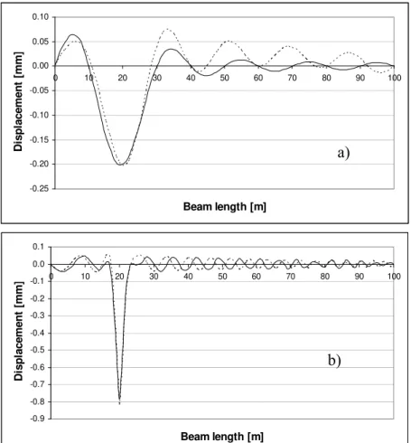
modes were implemented (Figure 3a)). For high number of modes, the results coincide with the full integration method, thus there is no way how to remove in ANSYS the numerical error.

-0.25 -0.20 -0.15 -0.10 -0.05 0.00 0.05 0.10

0 10 20 30 40 50 60 70 80 90 100

Beam length [m]

D

ispl

ace

m

e

nt

[

m

m

]

-0.9 -0.8 -0.7 -0.6 -0.5 -0.4 -0.3 -0.2 -0.1 0.0 0.1

0 10 20 30 40 50 60 70 80 90 100

Beam length [m]

D

is

p

la

c

e

m

e

n

t [m

m

]

Figure 3: Error in transient solution with mode superposition solution method implemented, ANSYS (dotted curve) and MAPLE (full curve): a) 10 modes

implemented, b) 500 modes implemented.

It can therefore be concluded that the results here presented are obtained faster and in a more accurate way, than the ones obtained by standard finite element codes.

2.2 Governing equations and simplifying assumptions

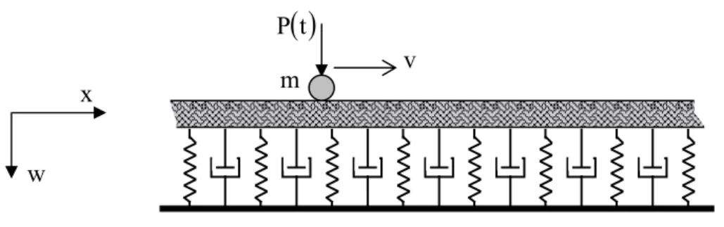
Let a uniform motion of a time variable vertical force along a horizontal finite beam on a linear visco-elastic foundation be assumed (Fig. 4). The foundation is modelled as distributed spring-and-dashpot sets. Simplifications for the analysis of vertical vibrations are outlined as follows:

(i) the beam obeys linear elastic Euler-Bernoulli theory;

(ii) the beam damping is proportional to the velocity of vibration. a)

Figure 4: Structure under consideration.

Taking into account the assumptions stated above, the equation of the forced vibration w(x,t) reads as [11]:

( )

( )

( )

( ) ( ) ( ) ( ) ( )

(

) ( )

( )

,

t t , x w m t P vt x

t , x w x k t

t , x w x c t

t , x w x x

t , x w x EI x

2 2 2

2

2 2

2 2

⎟⎟ ⎠ ⎞ ⎜⎜

⎝ ⎛

∂ ∂ − −

δ

= +

∂ ∂ + ∂ ∂ μ + ⎟⎟ ⎠ ⎞ ⎜⎜

⎝ ⎛

∂ ∂ ∂

∂

(1)

where EI represents the flexural rigidity, μ the mass per unit length, c the damping coefficient and k Winkler constant. w stands for the transversal displacement, P for the travelling force and m for the mass of the load; w and P are considered positive when acting downwards. Further in Eq. (1): v is the constant velocity, x is the spatial coordinate, t is the time and δ is Dirac function. x has its origin at the left extremity of the structure. Zero time corresponds to force position at x=0. Characteristics EI, μ, c and k can have piece-wise constant distribution along the structure. It is assumed that there is only finite number of such discontinuities. Initial and boundary conditions are defined in a standard way. Velocity is maintained constant and no restriction is imposed on its magnitude.

3 Problem solution

Eq. (1) can be solved by normal-mode analysis [5, 11]:

( )

x,t q

( ) ( )

tw x

w _j

1 j

j

∑

∞

=

= . (2)

( )

t

q_j are the generalized coordinates of displacement and w_j

( )

x are the orthogonal natural modes normalised by:

( ) ( )

xw x dx

N 2_j

L

0

j =

∫

μ , (3)

( )

t P

v

x

w

where L it is the total length of the structure.

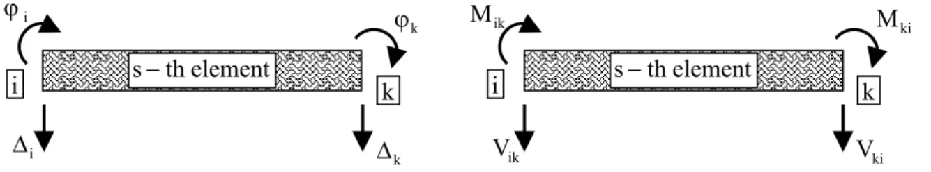
In order to calculate the undamped natural frequencies and the corresponding normal modes, structure is separated into structural elements with homogeneous properties. Each discontinuity in parameters EI, μ, k or c marks the beginning of a new structural element. Discontinuity in the damping coefficient c is obviously immaterial for undamped frequencies, however, later on in Eqs. (9) and (11) it will be seen, that this discontinuity must also be considered. Moreover, when the mass of the load is included, another structural node must be added. This one is the most difficult to handle because it varies its position in time. Then the load mass is included in the place of discontinuity as an additional concentrated mass element. On the contrary to the finite elements, only as many as elements, as the number of discontinuities indicates are needed, because the normal modes can be determined exactly within each structural element. In Fig. 5 the degrees of freedom and the member-end generalized harmonic forces are shown.

Figure 5: Degrees of freedom and member-end generalized harmonic forces of the s-th structural element wis-th nodes i and k.

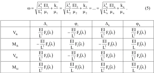
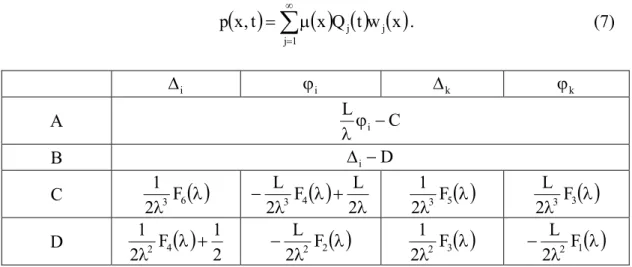
Let the full structure be separated into n structural elements. The local dynamic stiffness matrix of clamped-clamped s-th structural element is given in Table 1 (compare with Fig. 2). It is composed by amplitudes of member-end generalized harmonic forces of the element under steady-state vibration exited by harmonic motion of element nodes with a given circular frequency ω. Terms in Table 1 exploit Kolousek’s functions [8]:

( )

1 cos cosh sin sinh F s s s s s s

1 _{λ λ −}

λ − λ λ − =

λ ,

( )

1 cos cosh cos sinh sin cosh F s s s s s s s s

2 _{λ λ −}

λ λ − λ λ λ − = λ ,

( )

1 cos cosh cos cosh F s s s s 2 s s

3 _{λ λ −}

λ − λ λ − =

λ ,

( )

1 cos cosh sin sinh F s s s s 2 s s

4 _{λ λ −}

λ λ λ

=

λ , (4)

( )

1 cos cosh sin sinh F s s s s 3 s s

5 _{λ λ −}

λ + λ λ

=

λ ,

( )

1 cos cosh cos sinh sin cosh F s s s s s s 3 s s

6 _{λ λ −}

λ λ + λ λ λ − = λ .

Parameters λ_s, of different elements are linked together with the excitation frequency as: ik M ki M ik

V V_ki

i s−thelement _k

i ϕ k ϕ i Δ k Δ

n n n n 4 n 4 n 2 2 2 2 4 2 4 2 1 1 1 1 4 1 4

1 EI k

L ... k EI L k EI

L μ +μ

λ = = μ + μ λ = μ + μ λ =

ω . (5)

i

Δ ϕi Δk ϕk

ik

V ₃ F₆

( )

λ

L

EI ₋

_{( )}

_λ

4 2 F L

EI

_{( )}

_λ

5 3 F L

EI

_{( )}

_λ

3 2 F L EI

ik

M − ₂ F₄

( )

λ

L

EI

_{( )}

λ 2 F L

EI

_{( )}

λ − ₂ F₃

L

EI

_{( )}

λ 1 F L EI ki

V ₅

( )

λ

3 F L

EI

_{( )}

λ − ₂ F₃

L

EI

_{( )}

λ 6 3 F L

EI

_{( )}

λ 4 2 F L EI ki

M ₂ F₃

( )

λ

L

EI

_{( )}

λ 1 F L

EI

_{( )}

λ 4 2 F L

EI

_{( )}

λ 2 F L EI

Table 1: Amplitudes of member-end generalized harmonic forces of the s-th structural element with nodes i and k. Subscript s applies to all parameters, but it is

omitted for the sake of simplicity.

The global dynamic stiffness matrix is assembled in a standard way by the direct stiffness method and its determinant is set to zero. Roots of this equation, ω_j, correspond to the natural frequencies. Substituting ω=ω_j back into the global matrix, unknown displacements and rotations at structural nodes can be calculated.

Normal modes are functions composed by well-defined parts within each structural element and linked together by the nodal displacements and rotations. The natural undamped j-th mode of vibration in the s-th structural element reads as:

( )

(

)

(

)

(

)

(

)

n ,... 2 , 1 s , L L x cosh D L L x sinh C L L x cos B L L x sin A x w s s 0 sj sj s s 0 sj sj s s 0 sj sj s s 0 sj sj sj = − λ + − λ + − λ + − λ = , (6)

where

∑

−

=

= s 1 1 r

r s

0 L

L and L_r is the length of the r-th structural element. Constants from Eq. (6) can be expressed as a function of the nodal displacements and rotations, their forms are given in Table 2.

( )

x,t

( ) ( ) ( )

x Q tw x

p j

1 j

j

∑

∞

=

μ

= . (7)

i

Δ ϕi Δk ϕk

A Lϕ_i−C

λ

B Δ_i−D

C

( )

λ

λ3 F6 2

1

_{( )}

λ + λ λ −

2 L F

2 L

4

3 λ3F5

( )

λ

2

1

_{( )}

λ λ3 F3 2

L

D

( )

2 1 F

2 1

4

2 λ +

λ − λ2 F2

( )

λ 2

L

_{( )}

_λ

λ2 F3 2

1

_{( )}

_λ

λ − ₂ F₁

2 L

Table 2: Constants of Eq. (6) for the s-th structural element with nodes i and k. Subscript s applies to all parameters. Within the context of normal modes, subscript j also applies to all parameters, except of L. Both subscripts are omitted for the sake

of simplicity. Here

( )

=

_∫

L

( ) ( )

0

j j t px,t w x dx

Q . (8)

For homogeneous initial conditions, it holds:

( )

₌

_{( )}

_∫

t

( )

_τ − μ( )( )( )−τ

(

_{( )(}

_−τ

₎

)

_τ

0

j t

x 2

x c

j j

j Q e sin b x t d

x b

1 t

q , (9)

where

( )

2

( )

_{( )}

2

j j

x 2

x c ω x

b _⎟⎟

⎠ ⎞ ⎜⎜

⎝ ⎛

μ −

= , (10)

which for concentrated force (point load) simplifies as:

( )

₌

_{( ) ( ) ( )}

_∫

t _{τ τ} − μ( )( )( )−τ

(

_{( )(}

_−τ

₎

)

_τ

0

j t

x 2

x c

j j

j P w v e sin b x t d

x b

1 t

q . (11)

linearly over each time interval

[

t_i−1,t_i

]

, where Δt=t_i−t_i−1 can be assumed constant, but it must be sufficiently small. Then an intermediate value within such interval reads as:

( )

( )

( )

( )

τ

Δ − + = τ − − t t Q t Q t Q

Q_{j j i 1} j i j i 1 , (12)

where τ is a local time starting at t_i−1. After some manipulations (in the following relations x-dependence is omitted for the sake of simplicity, value corresponding to the actual time must be used):

( )

(

(

)

(

)

)

₂

j , i i 2 j , i i j , i i j , i i t 2 c i j b t e b d t b sin E t b cos D e t

q = Δ + Δ + + Δ

Δ μ − ,

( )

( )

(

)

(

)

(

)

, b e t b cos E t b sin D e b b t e b d t q 2 c t q dt d 2 j , i i j , i i j , i i t 2 c j , i 2 j , i i 2 j , i i i j i j + Δ + Δ − + ⎟ ⎟ ⎠ ⎞ ⎜ ⎜ ⎝ ⎛ _Δ − − − μ − = Δ μ − (13) where

( )

i 1 j i Q t

d = ₋ ,

( )

( )

t t Q t Q

e_i j i j i 1

Δ −

= −

,

( )

₂

j , i i 1 i j i b d t q

D = ₋ − ,

( )

( )

3 j , i i j , i 1 i j 1 i j i b e b t q dt d 2 c t q E − + μ

= − − . (14)

Expressions presented in this section are rather simple; the difficulties arise in numerical expression of the results. Determination of natural frequencies is considered the most difficult part of the numerical assessment of the results expressed by Eq. (2). This difficulty is aggravated by the fact, that very high number of natural frequencies is required in problems with foundation discontinuity. After the global matrix has been assemblaged, Eq. (5) can be substituted, and the determinant can be expressed in terms of a single unknown, ω. Actually, it is more convenient to express the determinant in terms of ω2 and search for ω2 instead of

ω. Only numerical methods, can be used for roots search. The determinant has many singularities coincident with all natural frequencies of each structural element considered separately. The denominator consists of product of expressions: H₁

( )

λ₁ ,

1 cos

special treatment around the singularities, it is possible to solve the roots only in the nominator. Then software which can handle very large numbers and introduce high-digits precision must be used. Only in MAPLE (or similar symbolical calculation software) it is possible to: (a) increase digits precision without any link to the computed specified value; (b) deal with very high numbers. Therefore most of the procedures of numerical evaluation of the results were programmed in MAPLE environment, some of them could be placed also in MATLAB.

The methodology for extension to infinite beams by mitigation the boundary conditions effect is defined in the following way. It is assumed that the force starts to actuate at a length Li from the left support and that it varies from zero to its final value over an intermediate region Lc. The time variation of the force is assumed in a sinusoidal shape in order to keep the time derivatives continues. In more details:

( )

⎪ ⎪ ⎪ ⎩ ⎪ ⎪ ⎪ ⎨ ⎧ + > + ≤ < ⎟ ⎟ ⎠ ⎞ ⎜ ⎜ ⎝ ⎛ ⎟⎟ ⎠ ⎞ ⎜⎜ ⎝ ⎛ ⎟⎟ ⎠ ⎞ ⎜⎜ ⎝ ⎛ − − π + ≤ = v L L t for P v L L t v L for 2 1 L L L vt sin 1 2 P v L t for 0 t P c i 0 c i i c i c 0 i , (15)

where P0 is the final value of the force applied. This methodology ensures that the maximum displacement smoothly increases till its final value, which corresponds to the analytical maximum of the quasi-stationary regime. It would be possible to assume only linear variation of the force applied. Nevertheless, it was verified that if the time derivatives of the variation function are continues, it is better prevented possible oscillation of the final value. The question is how long Li and especially Lc should be. It is suggested and verified that analogy with a representative spring can be used. For the sake of simplicity it is assumed that the force applied increases linearly. Thus, let a ramped force with the maximum value F be applied on a mass m supported by a spring of the rigidity K. Time variation of the mass displacement can be expressed analytically by:

( )

(

)

_⎟⎟ ⎠ ⎞ ⎜ ⎜ ⎝ ⎛ ⎟⎟ ⎠ ⎞ ⎜⎜ ⎝ ⎛ − ⎟⎟ ⎠ ⎞ ⎜⎜ ⎝ ⎛ − + = t m K sin t t m K sin K t m F K F t u _c 3 c , (16)

3 c

c K

t m K cos 1 m 2

t

F ⎟

⎟ ⎠ ⎞ ⎜

⎜ ⎝ ⎛

⎟⎟ ⎠ ⎞ ⎜⎜

⎝ ⎛ −

. (17)

By implementation lower time tc, the amplitude gets generally higher, but there is an additional oscillation in the amplitude itself. For our purpose, it is enough to choose the time t_c, in a way to force the amplitude to a “reasonable” part of F/K. This requirement, as expected, does not depend on the force applied, but it does depend on m and K. In accordance with the analogy, K will be replaced by k and m by μ.

4 Case studies

4.1 Parametric

optimization

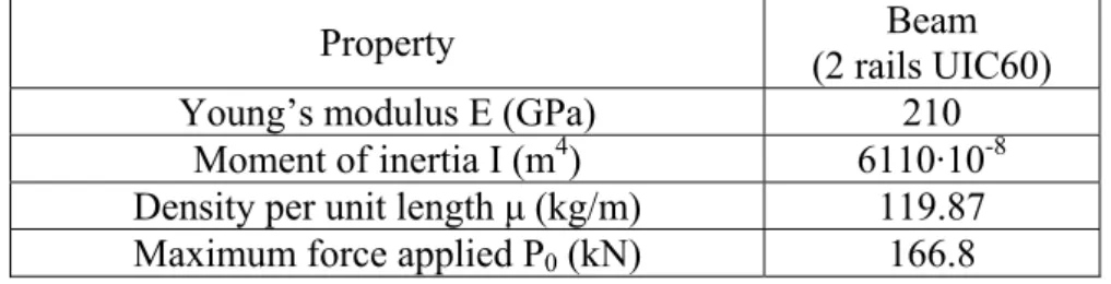
In this case study two UIC60 rails are used to model the beam. The load applied is approximated by the total axle mass of 17000kg corresponding to a locomotive of the Thalys high-speed train. A good isolation device and ideal rail surface is assumed, so that the harmonic component can be neglected and the load can be modelled as a constant moving force. All numerical input data are summarized in Table 3.

Property Beam

(2 rails UIC60)

Young’s modulus E (GPa) 210

Moment of inertia I (m4) 6110·10-8 Density per unit length μ (kg/m) 119.87 Maximum force applied P0 (kN) 166.8

Table 3: Numerical input data used in examples.

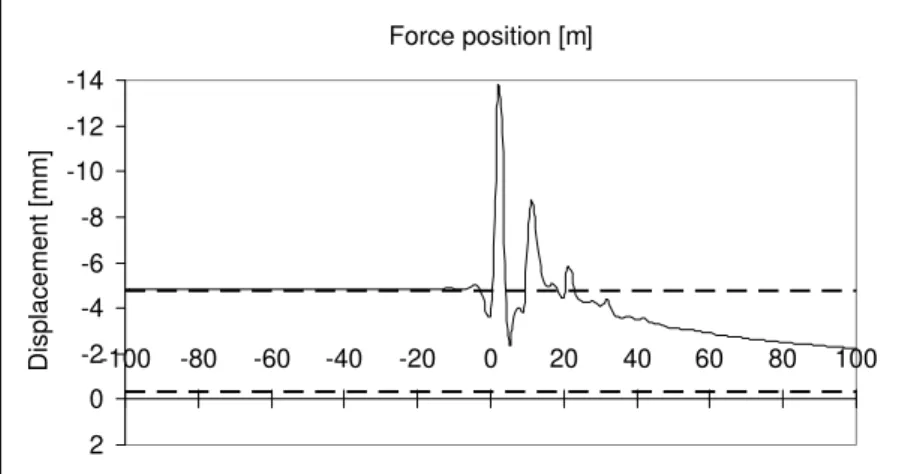
Analysis is performed in a parametric way with respect to the velocity and with respect to the intermediate foundation stiffness. During the analysis the velocity is varied by 10m/sfrom 140 to 160, to accommodate the chosen standard deviation. The maximum upward displacement was selected as the most harmful effect in this analysis. Evolution of this displacement with the load position is shown in Fig. 6 in the structure without an intermediate length. Regarding the passage forward, results of optimization show, that very small increase in foundation stiffness with respect to the soft value will attenuate the deflection wave propagation in the soft region and, at the same time, will ensure that the displacement shape is affected in the way that the next discontinuity in foundation stiffness does not cause the large peak in the response (Figs. 7 and 8).

-14

-12

-10

-8

-6

-4

-2

0

2

-100 -80 -60 -40 -20 0 20 40 60 80 100

Force position [m]

Displaceme

nt [mm]

Figure 6: Maximum upward displacement, passage forward by velocity v=150m/s, dashed lines are used for the quasi-stationary solutions.

-15 -10 -5 0 5 10 15 20 25 30 35

-10 -5 0 5 10 15

Beam length [m]

Displacement

[mm]

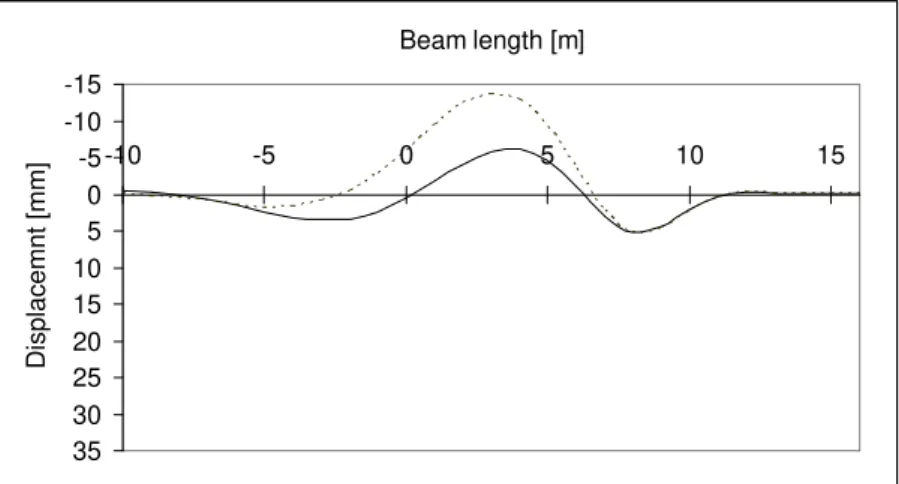
Figure 7: Displacement from the optimized solution (full curve) compared with the solution without the intermediate region (dotted curve), load position where the

-15 -10 -5 0 5 10 15 20 25 30 35

-10 -5 0 5 10 15

Beam length [m]

D

isplacem

n

t [mm]

Figure 8: Displacement from the optimized solution (full curve) compared with the solution without the intermediate region (dotted curve), load position where the

maximum in the non-optimized solution is achieved (load position at 8 m).

-16

-14

-12

-10

-8

-6

-4

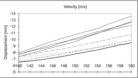
140 142 144 146 148 150 152 154 156 158 160

Velocity [m/s]

Displacem

ent [mm]

Figure 9: Maximum upward displacement as a function of velocity, passage forward. Bold curve shows the optimum solution (1400kN/m2), the closest values are for 1500kN/m2 (dashed), 1600kN/m2 (dotted), 1200kN/m2 (dot-and-dash line), other four full curves refer to 2000kN/m2, 3000kN/m2, 4000kN/m2, 8000kN/m2 (the

highest).

-14 -13

-12

-11

-10 -9

-8

-7

-6 -5

140 142 144 146 148 150 152 154 156 158 160

Velocity [m/s]

Dis

p

lace

ment [mm]

Figure 10: Maximum upward displacement as a function of velocity, passage backward. Bold curve shows the optimum solution (1500 kN m-2), the closest values

are for 1400 kN m-2 (dashed), 1600 kN m-2 (dotted), 1200 kN m-2 (dot-and-dash line), other four full curves refer to 2000 kN m-2, 3000 kN m-2, 4000 kN m-2, 8000

kN m-2 (the highest).

-15

-10

-5 0 5

10

15 20

25 30

-10 -5 0 5 10 15

Beam length [m]

Displacement

[mm]

Figure 11: Maximum upward displacement curves as a function of velocity, passage forward. Zero position is at the first discontinuity.

-10

0

10

20

30

40

50 -26 -21 -16 -11 -6 -1 4 9 14 19

Beam length [m]

Displaceme

n

t [mm]

The main advantage of this analysis is the fact, that the analytical solution is used, therefore in each studied case only a small region before and after the intermediate region can be analysed to find the maximum. 10m-length is enough for the passage forward, slightly more is necessary for the passage backward (20m-length was used).

Maximum upward displacement [mm]

Passage forward (150 m s-1)

Passage backward (150 m s-1)

No intermediate part 13.72 10.83

Intermediate stiffness

1400 kN m-2 6.92 8.13

Intermediate stiffness

1500 kN m-2 7.42 7.77

Table 4: Maximum upward displacement for the passage by the reference velocity. As a positive conclusion of this analysis is the fact, that the optimum intermediate stiffness for the forward and the backward passage are very similar, which is an important conclusion for practical use. In order to complete the optimization analysis, admissible values of 7 and 8mm for the upward displacement were chosen. The probability of their exceeding is summarized in Table 5. It can thus be concluded that the optimum intermediate stiffness in this problem is 1400 kN/m2 and the probability of exceeding the admissible displacements of 7 and 8mm is 70.7% and 30.4%, respectively.

Probability

Admissible value 8mm Admissible value 7mm Passage

forward

Passage

backward Total

Passage forward

Passage

backward Total Intermediate

stiffness 1400 kN/m2

1.0% 59.7% 30.4% 42.2% 99.3% 70.7% Intermediate

stiffness 1500 kN/m2

14.0% 31.9% 23.0% 79.9% 95.7% 87.8%

Table 5: Probabilities of exceeding the admissible values.

4.2 Effect of the mass of the load

-60 -50 -40 -30 -20 -10 0 10

0 0.02 0.04 0.06 0.08 0.1 0.12 0.14 0.16

Time [s]

D

is

p

la

c

e

m

e

n

t [m

m

]

Figure 13: Displacement at the free extremity of the beam with respect to time.

-8 -7 -6 -5 -4 -3 -2 -1 0 1

0 1 2 3 4 5 6 7 8

Beam length [m]

D

ispl

acem

ent

[

m

m

]

Figure 14: Deflection curve for the mass position at 3.8m. Results presented exactly match the expected ones presented in [12].

5 Conclusions and further development

The methodology presented has restrictions neither on velocity magnitude nor on damping. Load can be represented by a set of moving forces which magnitudes can be time dependent. Effect of the mass of the load can be included. Then normal modes must be evaluated at each time step and some of the previously mentioned advantages are lost.

Although focusing only on one-dimensional systems under physical and geometrical linearity this study provides an important insight into the problem of excessive ground vibrations induced by high-speed trains passing in sections where an abrupt change in vertical stiffness occurs. The methodology has some additional potentialities that will be explored in the future work. Among them it might be mentioned implementation of more complicated structural elements like an elevated railway, which can be modelled as a layered-beam system that is composed of two parallel beams with visco-elastic layer in between.

The results obtained have direct application in the analysis of railway track vibrations induced by high-speed trains when passing regions with significantly different foundation stiffness. The conclusions of this paper might be served as a design basis for the treatment of solution for such regions.

6 Acknowledgements

The first author would like to thank to Fundação para a Ciência e a Tecnologia, of the Portuguese Ministry of Science and Technology for supporting expenses related to this congress (grant PTDC/EME-PME/67658/2006: “Design of cellular elastomeric materials for passive vibration control”). The second author appreciates the support of the grant agency of the Czech Republic GA CR 103/08/1340.

References

[1] A.V. Metrikine, A.R.M. Wolfert, H.A. Dieterman, “Transition radiation in an elastically supported string. Abrupt and smooth variations of the support stiffness”, Wave Motion 27, 291-305, 1998.

[2] K.N. Van Dalen, Ground Vibration Induced by a High-Speed Train Running over Inhomogeneous Subsoil, Transition Radiation in Two-Dimensional Inhomogeneous Elastic Systems, Master Thesis, Department of Structural Engineering, TUDelft, 2006.

[3] K.N. van Dalen, A.V. Metrikine, “Transition radiation of elastic waves at the interface of two elastic half-planes”, Journal of Sound and Vibration 310, 702– 717, 2008.

[4] S.N. Verichev, A.V. Metrikine, “Instability of vibrations of a mass that moves uniformly along a beam on a periodically inhomogeneous foundation”, Journal of Sound and Vibration 260, 901-925, 2003.

[6] Z. Dimitrovová, J.N. Varandas, “Critical Velocity of a Load Moving on a Beam with a Sudden Change of Foundation Stiffness: Applications to High-Speed Trains”, Computers & Structures, in press, available on-line, DOI: 10.1016/j.compstruc.2008.12.005.

[7] Release 11 Documentation for MAPLE, Maplesoft a division of Waterloo Maple, Inc., 2007.

[8] Release R2007a Documentation for MATLAB, The MathWorks, Inc., 2007. [9] J.A. Cottrell, A. Reali, Y. Bazilevs, T.J.R. Hughes, “Isogeometric analysis of

structural vibrations”, Computer Methods in Applied Mechanics and Engineering 195, 5257-5296, 2006.

[10] Release 11.0 Documentation for ANSYS, Swanson Analysis Systems IP, Inc., 2007.

[11] L. Frýba, “Vibration of solids and structures under moving loads”. 3rd edition, Thomas Telford, London, 1999.