SENSITIVITY ANALYSIS OF TRACK VIBRATIONS DUE TO VERTICAL STIFFNESS VARIATION IN HIGH-SPEED RAILWAYS

Rethymno, Crete, Greece, 13–16 June 2007

SENSITIVITY ANALYSIS OF TRACK VIBRATIONS DUE TO

VERTICAL STIFFNESS VARIATION IN HIGH-SPEED RAILWAYS

Zuzana Dimitrovová1, José N. Varandas1, João R. de Almeida1, and Manuel A.G. Silva1

1

UNIC, Department of Civil Engineering New University of Lisbon, Monte Caparica, Portugal

{zdim,jnvs,jr,mgs}@fct.unl.pt

Keywords: High-speed trains, Foundation stiffness abrupt changes, Dynamic analysis, Tran-sient analysis, Methods of integral transformations.

1 INTRODUCTION

High speed trains, when crossing regions with abrupt changes in vertical stiffness of the track and/or subsoil, may generate excessive ground and track vibrations, ballast projections and increase the wheel, rail and track deterioration with negative impact on the vehicle stabil-ity and passengers comfort. Therefore specific methodologies must be established in order to determine these vibrations. Full understanding of these phenomena will lead to new construc-tion soluconstruc-tions and mitigaconstruc-tion of undesirable features.

Detailed information about these vibrations can be gathered from 3D finite element models. However, it is known that these analyses require very fine meshes to accurately capture the generated waves, giving rise to time consuming computation impractical for ordinary design. Analyses incorporating stiffness transitions necessitate more careful treatment in the region of the “discontinuity”, which naturally further increases the computing time.

First insight on these phenomena can be gained from simplified one-dimensional models. Steady-state analytical solutions of dynamic response of a beam on elastic or more complex foundation under moving loads are widely available [1, 2]. However, introduction of non-homogeneous properties of the system naturally requires transient response, for which avail-able results in the literature remain scarce.

In this paper, analytical transient solutions of dynamic response of one-dimensional sys-tems with sudden change of foundation stiffness are derived. Results are expressed in terms of vertical displacement. The problem is approached from the simplest level. First, a simply sup-ported beam is considered. Transient solution for moving force is extended to a beam on elas-tic foundation in Section 2. Dynamic response accounting for localized abrupt stiffness change is derived in Section 3 and sensitivity analysis of displacement at some chosen posi-tion with respect to stiffness is performed in Secposi-tion 4. Next, in Secposi-tion 5, the cantilever tran-sient solution is extended to account for elastic foundation and two cantilevers are joined together to form a clamped beam by imposing continuity conditions at the point of foundation stiffness change (Section 6). These results permit to study force passage through contiguous locations with different foundation stiffness. All presented results are confirmed using general purpose finite element code ANSYS. Graphs and numerical results are presented. Neverthe-less, it must be pointed out that, in order to obtain realistic dynamic response, vehicle spring-mass-damper system interacting with the rail track must also be considered. This point will be object of future research.

2 MOVING LOAD ON SIMPLY SUPPORTED BEAM ON ELASTIC FOUNDATION

The governing equation describing the dynamic response, under a constant moving load, P, of an Euler-Bernoulli’s beam in terms of displacements can be written as [3]:

( )

( )

_{( ) ( )}

P ct x t

t , x w 2

t t , x w x

t , x w

EI _{2 b}

2

4 4

− δ = ∂ ∂ μω + ∂ ∂ μ + ∂ ∂

. (1)

It is assumed that the beam follows linear elastic Hooke’s law, has constant cross-section

and constant mass per unit length, μ. As usual, small displacements, Navier’s hypothesis and

Saint-Venant’s principle are adopted. E, I and μ_b stand for Young’s modulus, moment of

speed, c. δ in equation (1) stands for the Dirac function. Denoting by L the total length of the beam, boundary and initial conditions read as:

( )

( )

( )

( )

x t , x w , 0 x t , x w , 0 t , L w , 0 t , 0 w L x 2 2 0 x 2 2 = ∂ ∂ = ∂ ∂ = = = = (2)

( )

( )

t t , x w , 0 0 , x w 0 t = ∂ ∂ = = (3)

Problem (1-3) can be solved by methods of integral transformations. First, Fourier sine fi-nite integral transformation is implemented and then Laplace-Carson integral transformation is applied, enabling to express the displacement in terms of sine series [3].

In order to account for the effect of elastic foundation, characterized by Winkler’s constant k, an additional term must be introduced into equation (1), which takes the following form:

( )

( )

( )

_{( ) (}

₎

EI _{2 b}

2 4 4 − δ = + ∂ ∂ μω + ∂ ∂ μ + ∂ ∂ (4)

The additional term changes the image of Laplace-Carson transformation. Nevertheless, basically the same procedure as in [3] can be used to obtain the final expression for the verti-cal displacements. In order to validate this procedure, an equivalent model was created using ANSYS software [4]. Element BEAM 54 of ANSYS library, with the capacity of introduction of elastic foundation, was used. Rayleigh damping was introduced by means of the coefficient

b 2ω =

α . Since ANSYS does not allow moving load implementation, for each time step a

new force position had to be considered according to the load speed and the element size. The computational results matched almost exactly the analytical solution, confirming the suitabil-ity of the strategy adopted for the analysis and suggesting that it is possible to solve numeri-cally other situations impossible to treat analytinumeri-cally.

Verification graphs are shown for representative cases, without attempt to adjust material

and geometrical properties to some real representation of railway track. Parameters ξ, ψ and ζ

can be introduced in order to characterize the magnitude of velocity, c, and the damping level,

b

ω . Thus, ξ and ζ stand for the ratio of circular frequency of the load, ω, and first circular

fre-quency of the free vibration of simply supported beam without, ω_{( )1} , and with, ω~_{( )1}, elastic

foundation. Similarly, ψ is the ratio between the damping circular frequency ω_b and ω_{( )1} . One

could then write:

( )1 ~ ω

ω =

ξ ,

( )1 b ω

ω =

ψ ,

( )1 ω

ω =

ζ , (5)

where: L

c π =

ω , _{( )}

μ π = ω EI L2 2

1 , ( ) _μ +_μ

π =

ω EI k

L ~

4 4

1 .

To assess the match between analytical and numerical results, a beam with L=10m,

EI=1000Nm2, P=1N and μ=0,06kg/m was considered. Several combinations of ξ, ψ and ζ

were chosen. In Figures 1 and 2, graphs for the cases ξ=0.476, ψ=0.5, ζ=0.5 and ξ=2, ψ=5,

ζ=2.1 are plotted for ten positions of the load along the beam length, namely at each precise

Figure 1: Vertical displacement for ξ=0.476, ψ=0.5 and ζ=0.5, plotted for 10 positions of the moving load (violet curve: analytical solution; blue curve: numerical results)

Figure 2: Vertical displacement for ξ=2, ψ=5 and ζ=2.1, plotted for 10 positions of the moving load (violet curve: analytical solution; blue curve: numerical results)

-0.0020 -0.0015 -0.0010 -0.0005 0.0000 0.0005

0 1 2 3 4 5 6 7 8 9 10

beam length [m]

ver

ti

cal

d

isp

lacemn

t [

m

]

ξ=2, ψ=5, ζ=2.1

-0.025 -0.020 -0.015 -0.010 -0.005 0.000 0.005

0 1 2 3 4 5 6 7 8 9 10

beam length [m]

ver

ti

cal

d

isp

lacemn

t [

m

]

3 MOVING LOAD ON SIMPLY SUPPORTED BEAM ON ELASTIC

FOUNDATION WITH LOCALIZED CHANGE IN VERTICAL STIFFNESS

In this case it is necessary to add an additional term to Equation (4) in the following way:

( )

( )

( )

_{( ) (}

₎

_{( ) (}

_)P

ct x t , x w k x x t , x kw t t , x w 2 t t , x w x t , x w

EI _{2 b 0 0}

2 4 4 − δ = − δ + + ∂ ∂ μω + ∂ ∂ μ + ∂ ∂ (6)

where x corresponds to the position of the sudden stiffness change and ₀ k stands for the ad-₀

dition of Winkler’s constant at the position x . Therefore, this effect corresponds to the intro-₀

duction of a discrete elastic spring. Although it is impossible to solve Equation (6) exactly, an approximate solution is proposed herein using an approach similar as another described in [3] for a different context. It is assumed that:

( )

( )

= (7)

where W(j,t) stands for the image of w(x,t) in Fourier sine finite integral transformation. After merging Equation (7) into (6), the procedure to obtain the final solution is similar to the one described in previous section. It can then be written:

( )

_∑

( )

w (8)

where

( )

(

)

(

)

(

)

_{( )}

(

)

_{( )}

₍

_{( )}

_{( )}

₎

− _{sin bt 2acosct e cosbt}

e b c a b ct sin c c b a c a 4 c b a Pc t , j W at at 2 2 2 2 2 2 2 2 2 2 2 2 , (9) and

( )−ω + _μ π = ω

ω = ω

= ), c j

L x j ( sin L k 2 ~ b ,

a 2 0 2 0

b 2

j

b . (10)

Obviously, when k =0, Equations (8-10) reduce to the problem (1-3) addressed in the pre-₀

vious section.

Analytical (approximate) results according to (8-10) were compared with numerical ones.

Significant increase in elastic foundation from _k=_1N/m2 _{to localized}

0

k =1000N/m at

posi-tion Lx₀ =0.3 was considered. To measure this localized effect, parameter κ is introduced:

kL

k₀

=

κ . (11)

Keeping the definition of parameters ξ, ψ and ζ from previous section, the case for ξ=2, ψ=0.5,

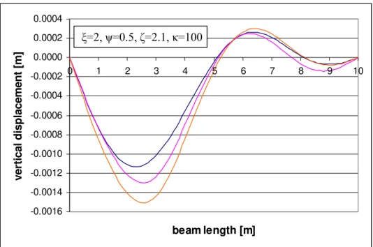
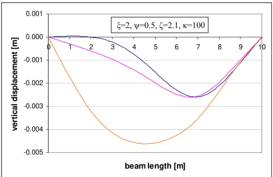
ζ=2.1 and κ=100 is presented in the graphs depicted in Figures 3, 4 and 5. For the sake of

comparison, the analytical solution for the case without k introduction (orange curve) is also ₀

in-crease); at 0.3L (coincident with the localized stiffness increase) and at 0.7L (after the local-ized stiffness increase).

Figure 3: Vertical displacement for ξ=2, ψ=0.5, ζ=2.1 and κ=100, plotted at the position 0.2L of the moving load (blue curve: numerical results; violet and orange curves: analytical solutions with and without k0, respectively)

Figure 4: Vertical displacement for ξ=2, ψ=0.5, ζ=2.1 and κ=100, plotted at the position 0.3L of the moving load (blue curve: numerical results; violet and orange curves: analytical solutions with and without k0, respectively)

-0.0010 -0.0008 -0.0006 -0.0004 -0.0002 0.0000 0.0002

0 1 2 3 4 5 6 7 8 9 10

beam length [m]

ver

ti

cal

d

isp

la

cemen

t [

m

]

ξ=2, ψ=0.5, ζ=2.1, κ=100

-0.0016 -0.0014 -0.0012 -0.0010 -0.0008 -0.0006 -0.0004 -0.0002 0.0000 0.0002 0.0004

0 1 2 3 4 5 6 7 8 9 10

beam length [m]

ver

ti

cal

d

isp

lacemen

t [

m

]

Figure 5: Vertical displacement for ξ=2, ψ=0.5, ζ=2.1 and κ=100, plotted at the position 0.7L of the moving load (blue curve: numerical results; violet and orange curves: analytical solutions with and without k0, respectively)

It is seen that the high value of k does not cause any irregularity in the vertical deflection ₀

profile; in fact, maximum deflection is lower than in the original case, due to the fact that k ₀

works as an additional flexible beam support, reducing the “beam span”. However, this is not in accordance with what is experienced by real rail vehicles. One of the obvious reasons for this discrepancy is that in such cases interaction of spring-mass-damper system of the vehicle with the beam structure cannot be omitted. Nevertheless, it is observed that the approximate analytical solution agrees reasonably with the numerical one. This allows for direct sensitivity analysis and, in the other hand, making the beam sufficiently long, conclusions can be drawn for real situations, without influence of the support conditions.

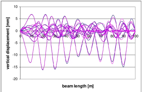
In order to evaluate the efficiency of this solution, a case approaching real conditions is analysed. It is assumed that the beam corresponds to the full superior structure of a railway track, including rails, sleepers, ballast and sub-ballast. Dimensions of the beam cross-section

equal to 4m×1m, material properties E=200MPa, ρ=1800kg/m3 and a load P=100kN moving

at constant velocity c=45,3m/s=163,2km/h are adopted. Beam length is extended to 100m and

Winkler’s constant is taken as 200kN/m2. Actually this value is quite a low estimate for a real

soil. The reason for this is that the numerical solution becomes unreliable for very strong

foundation, because then first natural frequencies, ω~_{( )j}, are very similar and this can disorder

their sequence and consequently attribute different weight to waves forms in transient solution. Analytical solution is more stable numerically, nevertheless, significant number of sine series must be taken into account. Results were calculated by computer package Matlab [5] where 1000 series members were implemented. Analytical and numerical values fit well, as shown in Figure 6. However, the assumption subjacent to Equation (7) for localized stiffness increase is approximate and the coincidence of numerical and analytical values may be occasional. Hence, further research is needed in order to validate and improve this approach.

-0.005 -0.004 -0.003 -0.002 -0.001 0.000 0.001

0 1 2 3 4 5 6 7 8 9 10

beam length [m]

ver

ti

cal

d

isp

la

cemen

t [

m

]

-20 -15 -10 -5 0 5 10

0 10 20 30 40 50 60 70 80 90 100

beam length [m]

ver ti ca l d isp lacemen t [ m m]

Figure 6: Vertical displacement for c=45,3m/s, no damping and k=200kN/m2, plotted for 10 positions of the moving load P=100kN

(violet curve: analytical solution; blue curve: numerical results)

At the present, extension of results to consider harmonic loads, multiple loads, other types of damping and simplified vehicle models are under development.

4 SENSITIVITY ANALYSIS OF DYNAMIC RESPONSE OF MOVING LOAD ON SIMPLY SUPPORTED BEAM ON ELASTIC FOUNDATION WITH

LOCALIZED ABRUPT CHANGE IN VERTICAL STIFFNESS

All derivatives of solution (8-10) can be done in an analytical way. For instance:

( )

_∑

( )

k , (12)

( )−ω +_μ+ _μ ⎜_⎝⎛ π ⎟_⎠⎞

ω

⎟ ⎠ ⎞ ⎜ ⎝ ⎛ π μ

= ∂

∂

L x j sin L

k 2 k

L x j sin L

1

k b

0 2 0 2

b 2

j

0 2

0

. (14)

Implementation of equations presented above is straightforward.

5 MOVING LOAD ON CANTILEVER BEAM ON ELASTIC FOUNDATION

In order to study sudden elastic foundation stiffness change, implemented in whole region, cantilever dynamic response must be extended to account for elastic foundation. Then two cantilever solutions, corresponding to beams clamped on left and right hand side, with differ-ent value of Winkler constant can be connected together by continuity conditions.

General expression of transient vertical displacement of beam with various boundary con-ditions subjected to a moving load can be written in the following form, [3]:

( )

( )

( )

t , x

w _j

1

j j

∑

=

μ

= , (15)

where

( )

( )

L x cosh C L

x sinh B L

x cos A L

x sin x

w _j = λj + _j λj + _j λj + _j λj (16)

and

( )

( )

∫

0 2

j

j w xdx

W . (17)

Constants from equation (16), λ_j, A , _j B , _j C , must be determined numerically in order to _j

satisfy given boundary conditions. Irrespectively of the beam being clamped on the right or on

the left hand side, λ_j correspond to roots of the following equation:

0 cosh cos

1+ λ_j λ_j= (18)

and A is calculated from: _j

j j

j j

j

cosh cos

sinh sin

A

λ + λ

λ + λ −

= . (19)

Then for right clamping C_j=A_j, jB_j=1∀ and for left clamping C_j=−A_j, jB_j=−1∀ .

Governing equation is again Equation (4) and the natural frequencies are given by:

( )= λπ _μ

ω EI

L4

4 4

j

j , ( ) _μ +_μ

π λ =

ω EI k

L ~

4 4 4

j

j (20)

for beams without and with elastic foundation, respectively.

The free end of the cantilever must allow introduction of non-zero vertical force and mo-ment, which will correspond to transversal force and bending moment of the full clamped

( )

∫

(

( )

(

)

)

(

(

)

)

0

t a

j c EIz0,L, e sin b t d Pw

b 1 t , j

W , (21)

where

(

)

( )

( )

( )

( )

(

)

( )

( )

( )

( )

0 x j j

dx x dw

EI t , L M L w EI

t , L V t , L , 0 z

, dx

x dw

EI t , 0 M 0 w EI

t , 0 V t , L , 0 z

= =

+ −

=

− =

(22)

for right and left clamping, respectively, and

( ) 2b 2

j b

~ b ,

a=ω = ω −ω . (23)

For the sake of comparison, similar parameters as in Section 2 are introduced according to:

L c 1 λ =

ω ,

( )1 ~ ω ω =

ξ ,

( )1 b ω

ω =

ψ ,

( )1 ω

ω =

ζ (24)

with Equation (20) implemented. Verification of derived formulas was again performed in ANSYS. Moving load and/or prescribed variation of free end internal forces was tested. In every case analyzed, the match between analytical and numerical solutions was excellent.

6 MOVING LOAD ON CLAMPED BEAM ON ELASTIC FOUNDATION WITH SUDDEN DROP IN VERTICAL STIFFNESS

In order to model the dynamic response of a clamped beam with sudden drop/increase in vertical stiffness, two cantilever solutions, corresponding to beams clamped on left and right hand side, with different value of Winkler constant are connected together by continuity con-ditions. The point of Winkler constant discontinuity corresponds to the point of beam continu-ity, therefore equilibrium of internal forces must be preserved and equality of vertical displacement and of its spatial derivative (rotation) must be maintained at that point. The in-ternal forces (the unknowns) can be simply introduced by same values in both clamped beam solutions and solved from the equations imposing continuity of vertical displacement and ro-tation at the point of Winkler constant discontinuity.

Solution of this problem is not straightforward and must be done numerically, although pa-rameters dependence is preserved. In more detail, the main difficulty lies in Equation (21), where the function z, given by (22) must be integrated over time when the actual time varia-tion of internal forces is unknown. Nevertheless, linear variavaria-tion can be assumed within each time step. Then, in the way described above, internal forces can be solved at each time step

and, obviously, values Vi and Mi for i=1,…,n can be used to determine piecewise linear

dis-tribution and to calculate Vn+1 and Mn+1. Unfortunately none of the previous integrations can

be used in next time step, due to the convolution form of the integral.

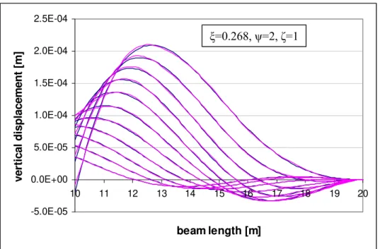
switched their role. Coincidence of results is again very good. In Figures 7 to 9, graphs of de-flection curves calculated numerically and recovered analytically are shown. For the sake of

simplicity, only the following cases are presented: ξ=ζ=1 and ψ=0 for positions of the load at

0.1, 0.2,…, 1m and results on the right hand side; ξ=ζ=1 and ψ=0 for positions of the load at 1,

1.1, 1.2, …, 2m and results on the left hand side; ξ=0.268, ψ=2 and ζ=1 for positions of the

load at 1, 1.1, 1.2, …, 2m and results on the right hand side.

Figure 7: Vertical displacement for ξ=1, ψ=0 and ζ=1, plotted for 10 positions of the moving load from 0 to 1m (violet curve: analytical solution; blue curve: numerical results)

Figure 8: Vertical displacement for ξ=1, ψ=0 and ζ=1, plotted for 11 positions of the moving load from 1 to 2m (violet curve: analytical solution; blue curve: numerical results)

-2.0E-03 -1.5E-03 -1.0E-03 -5.0E-04 0.0E+00 5.0E-04

0 1 2 3 4 5 6 7 8 9 10

beam length [m]

ver

ti

cal

d

isp

la

cemen

t [

m

]

ξ=1, ψ=0, ζ=1 -2.E-05

-5.E-06 5.E-06 2.E-05 3.E-05 4.E-05

10 11 12 13 14 15 16 17 18 19 20

beam length [m]

ver

ti

cal

d

isp

lacemen

t [

m

Figure 9: Vertical displacement for ξ=0.268, ψ=2 and ζ=1, plotted for 11 positions of the moving load from 1 to 2m (violet curve: analytical solution; blue curve: numerical results)

7 CONCLUSIONS

In this paper, analytical transient solutions of dynamic response of one-dimensional sys-tems with sudden change of foundation stiffness are derived. Abrupt localised in-crease/decrease is solved approximately, sudden drop/increase in foundation stiffness valid in whole region is solved exactly. However, assumptions about time variation of internal forces at the section of discontinuity must be adopted and the analytical solution will include nu-merical procedure. In both cases, results are expressed in terms of vertical displacement. Sen-sitivity analysis of the response amplitude is also performed. The analytical formulation for this problem, to the authors’ knowledge, has not been published yet. Although related to one-dimensional cases, this study can give first insight into the problem of excessive ground vi-brations caused by high speed trains crossing regions with abrupt changes in vertical stiffness of the track and/or subsoil.

REFERENCES

[1] M. Shamalta, A.V. Metrikine, Analytical study of the dynamic response of an

embed-ded railway track to a moving load. Archive of Applied Mechanics, 73, 131-146, 2003.

[2] A.V. Vostroukhov, A.V. Metrikine, Periodically supported beam on visco-elastic layer

as a model for dynamic analysis of a high-speed railway track. International Journal of

Solids and Structures, 40, 5723-5752, 2003.

[3] L. Frýba, Vibration of solids and structures under moving loads, 3th Edition. Thomas

Telford, 1999.

[4] Release 10.0 Documentation for ANSYS, Swanson Analysis Systems IP, Inc., 2006.

-5.0E-05 0.0E+00 5.0E-05 1.0E-04 1.5E-04 2.0E-04 2.5E-04

10 11 12 13 14 15 16 17 18 19 20

beam length [m]

ver

ti

cal

d

isp

la

cemen

t [

m

]