Abstract
In this paper analytical transient solutions of dynamic response of one-dimensional systems with sudden change of foundation stiffness are derived. In more details, cantilever dynamic response, expressed in terms of vertical displacement, is extended to account for elastic foundation and then two cantilever solutions, corresponding to beams clamped on left and right hand side, with different value of Winkler constant are connected together by continuity conditions. The internal forces, as the unknowns, can be introduced by the same values in both clamped beam solutions and solved. Assumption about time variation of internal forces at the section of discontinuity must be adopted and originally analytical solution will have to include numerical procedure.
Keywords: high-speed trains, induced vibration, foundation stiffness abrupt changes, dynamic analysis, transient analysis, vehicle-rail-track interaction, methods of integral transformations, analytical solution, numerical analysis, commercial software.
1 Introduction
Mathematical representation of more or less complicated physical occurrences represents the framework of scientific and engineering community. Among the vast number of distinct technological demands that civil and mechanical engineering has to deal with, the one focused on the development and the improvement of transportation design is certainly one of the most challenging.
The systematic growth of high-speed lines and the rapid evolution of train vehicles capable to reach more than 500km/h in test operation (TGV - France) gave raise to a number of specific related problems and consequently motivated a significant amount of scientific work. Some of the most demanding issues are: (i) attenuation of ground-borne vibrations when train traffic passes nearby residential
Ground Vibrations Induced by
High-Speed Trains in Regions with
Sudden Foundation Stiffness Change
Z. Dimitrovová, J. Varandas and M.A.G. Silva
Department of Civil Engineering
New University of Lisbon, Monte da Caparica, Portugal
areas; (ii) critical velocity analyses particularly pertinent when train lines have to cross soft soil areas; (iii) novel solutions guaranteeing low maintenance cost.
This paper concerns with excessive ground and track vibrations induced by high speed trains, when crossing regions with abrupt changes in vertical stiffness of the track and/or subsoil. These vibrations have been observed and recorded, they degrade rolling equipment and track and raise questions related to the vehicle stability and passengers comfort. Vertical stiffness change can be caused by foundation inhomogeneity or by modification of structural solutions. In the latter case, covering passage from bridge or tunnel to regular line and transition from ballasted to concrete slab track and vice versa, the vertical stiffness change can be quite sharp and representative values can differ by several orders. These scenarios have been already studied numerically and soil improvement solutions, attempting to gradually connect the different regions, are presented in [1].
Mathematical representation of induced vibrations can be done by simplified analytical models. They permit to obtain estimates of the dynamic system response to a moving load travelling over a supporting structure, laid on a foundation half-space. The review made by Hung and Yang [2] gives some historical overlook, referring the pioneering work of Lamb [3] where the classical Lamb’s problem of a point or line load acting on the surface of elastic half-space is solved. However, movement of the load is not yet considered.
A wide variety of analytical and semi-analytical solutions, accounting for moving load, is presently available in the literature. Obviously, analytical exact solutions for such a complex physical phenomena can only be achieved with a significant amount of physical and geometrical simplifications. One of the most common one is the attempt to replace the visco-elastic half-space by an equivalent elastic foundation, which can be in the simplest case represented by Winkler constant. Then the track is accessed by Euler-Bernoulli beam, over which the load travels. This problem was first solved by Timoshenko [4] and is also presented by Frýba [5], together with additional developments and practical applications. Complex two-dimensional design is presented in [6].
As noticed by Metrikine and Popp [7], the assumption of constant stiffness to model the support reaction to moving load is questionable. The moving load generates elastic waves travelling inside the surrounding soil that interacts with sleepers reaction intended to simulate. In this work the authors derived expression for the equivalent Winkler type stiffness of a visco-elastic half-space as a function of natural frequencies of the beam and of the phase shift of vibrations of neighbouring sleepers. With this formulation it is possible to replace the half-space by a set of springs with equivalent complex stiffness, in which the imaginary part arises due to radiation of waves into the half-space. The same concept is used in [8-9].
Nevertheless, except for [1], the above mentioned works do not concern with sudden vertical stiffness change and corresponding aggravated vibrations. Detailed information about these vibrations can be gathered from three-dimensional finite element models. However, it is known that these analyses require very fine meshes to accurately capture the generated waves, giving rise to time consuming computation impractical for ordinary design. Analyses incorporating stiffness transitions necessitate more careful treatment in the region of the “discontinuity”, which naturally further increases the computing time.
First insight on aggravated vibrations due to vertical stiffness sudden change can be gained from simplified one-dimensional models. Introduction of non-homogeneous properties of the system naturally requires transient response, for which available results remain scarce in the presently available bibliography.
In this paper analytical transient solutions of dynamic response of one-dimensional systems with sudden change of foundation stiffness are derived. Results are expressed in terms of vertical displacement. The problem is approached from the simplest level. First, in Section 2, general transient dynamic solution for beam subjected to moving force from [5] is extended to account for elastic foundation and damping. Expressions for vertical displacement are particularized for simply supported and clamped beam and left and right cantilevers with non-homogeneous static boundary conditions. Then, in Section 3, two cantilever solutions, corresponding to beams clamped on left and right hand side, with different value of Winkler constant are joined together by continuity conditions. Point of Winkler constant discontinuity corresponds to point of beam continuity, therefore equality of internal forces must be preserved and equality of vertical displacement and of its spatial derivative must be maintained. Then internal forces, as the unknowns, can be simply introduced by same values in both clamped beam solutions and solved from the equations mentioned above. Assumption about time variation of internal forces at the section of discontinuity must be adopted and originally analytical solution will have to include numerical procedure. These results permit to study force passage through continuous locations with different foundation stiffness. All presented results are programmed in software Matlab [16] and confirmed using general purpose finite element code ANSYS [17]. Graphs and numerical results are presented. Nevertheless, it must be pointed out that, in order to obtain realistic dynamic response, vehicle spring-mass-damper system interacting with the rail track must also be considered. This issue is the object of future research.
Some developments make part of research project “Response of system railway track-soil to loads imposed by high speed trains” POCI/ECM/61114/2004, founded by Portuguese supporting research entity (Fundação para a Ciência e a Tecnologia).
2 Problem statement
foundation, either simple supports or clamped ends can be assumed at extremities. Simple supports are easier to deal with, because modes of natural undamped vibrations can be expressed in sine series. Beams must be modelled with sufficient length in order to eliminate the effect of chosen boundary conditions.
2.1 Case
studies
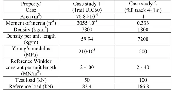
Two case studies, according to two possible distinct approaches, are chosen. In Case study 1 beam represents one standard rail UIC60 and thus the elastic foundation has to represent the flexibility of the full railway track and corresponding foundation. In Case study 2 beam involves the full superior structure of a railway track, including rails, sleepers, ballast and sub-ballast and therefore the elastic foundation corresponds only to the subgrade effect. Obviously both cases are quite far from reality, but they can give some feelings about the involved phenomena. Numerical data used in case studies are summarized in Table 1.
Property/ Case
Case study 1 (1rail UIC60)
Case study 2 (full track 4×1m)
Area (m2) 76.84·10-4 4
Moment of inertia (m4) 3055·10-8 0.333
Density (kg/m3) 7800 1800
Density per unit length
(kg/m) 59.94 7200
Young’s modulus
(MPa) 210·10
3
200 Reference Winkler
constant per unit length (MN/m2)
2 -100 2 - 40
Test load (kN) 50 100
Reference load (kN) 83.4 166.8
Table 1: Numerical data used in case studies.
Figure 1: Elastic spring forces from three-dimensional analysis.
Figure 2: Elastic spring force evolution over time (violet curve: analytical estimate; blue curve: numerical results).
Then elastic force distribution was analyzed over time. It resembles soil reaction of beam on elastic foundation, studied in [5]. Maximum peak and curve opening in time were considered as decisive parameters in order to define a reference Winkler constant. Following [5], same curve opening can be obtained if the beam,
-0.5 -0.4 -0.3 -0.2 -0.1 0.0 0.1
0 1 2 3 4 5 6
Model length (m) Elastic spring force (N)
-0.4 -0.3 -0.2 -0.1 0.0 0.1
0 0.05 0.1 0.15 0.2 0.25
corresponding to the rail, is posed on elastic layer with 100MN/m2 Winkler constant. Comparison of analytical estimate with numerical solution is presented in Figure 2.
Estimates for Case study 2 are summarized in internal report [19].
2.2 Finite beam on elastic foundation subjected to moving load
The governing equation describing the dynamic response, under a constant moving load, P, of an Euler-Bernoulli’s beam in terms of displacements can be written as [5]:
( )
( )
( ) (
)
P vt x t t , x w 2 t t , x w x t , x wEI 2 b
2 4 4 − δ = ∂ ∂ μω + ∂ ∂ μ + ∂ ∂ . (1)
It is assumed that the beam follows linear elastic Hooke’s law, has constant cross-section and constant mass per unit length, μ. As usual, small displacements, Navier’s hypothesis and Saint-Venant’s principle are adopted. E, I and μb stand for Young’s modulus, moment of inertia and circular frequency of damping, respectively; w represents the vertical deflection measured from equilibrium position and oriented downwards, x is spatial coordinate measured from left to right end of the beam and t is the time. δ in equation (1) stands for the Dirac function. It is also assumed that the mass of the load is small compared with the mass of the beam and that the load moves with constant speed, v. This assumption is obviously neither fulfilled in Case study 1 nor in Case study 2. Accounting for the mass of the load into calculations is currently under development.
In order to include the effect of elastic foundation, characterized by Winkler’s constant k, an additional term must be introduced into Equation (1):
( )
( )
( )
( ) (
)
P vt x t , x kw t t , x w 2 t t , x w x t , x wEI 2 b
2 4 4 − δ = + ∂ ∂ μω + ∂ ∂ μ + ∂ ∂ . (2)
The problem can be solved by methods of integral transformations, namely expansion in series given by Equation (3), i.e. general method of finite integral transform is applied first, and then Laplace-Carson transformation is implemented. General expression of transient vertical displacement of beam with various boundary conditions subjected to a moving load can be thus written in the following form, [5]:
( )
∑
∞( )
( )( )
= = 1 j j j W x w t , j W t , xw , (3)
where w( )j
( )
x stand for beam natural undamped normal vibration modes, given by:( )
( )
L x cosh C L x sinh B L x cos A L x sin xand =
∫
μ ( )( )
L
0 2
j j w x dx
W . (5)
je to vlastne norma na druhou
Constants from Equation (4), λj, A , j B , j C , must be determined from given j boundary conditions.
If boundary conditions are homogeneous and initial conditions, given bellow, as well:
( )
( )
0t t , x w , 0 0 , x w 0 t = ∂ ∂ = = , (6)
the image of Laplace-Carson transformation can be expressed as:
( )
( ) ( )( )
( ) ( )(
)
(
)
∫
−= t − −
0 j τ t a j j dτ τ t b sin e vτ Pw b 1 t j,
W , (7)
where a=ωb,b( )j = ω2( )j −ωb2 . Here ω( )j stand for j-natural frequency of the beam calculated by:
( ) μ +μ
λ =
ω EI k
L4
4 j
j . (8)
Next equation defines critical velocity and critical damping case by:
( ) 1 1 = ω ω = ξ , ( ) 1 1 b = ω ω =
ζ , (9)
where ω expresses frequency of the load in the following way:
L v λ
ω= 1 . (10)
Homogeneous boundary conditions of simply supported beam are:
( )
( )
( )
( )
0,x t , x w , 0 x t , x w , 0 t , L w , 0 t , 0 w L x 2 2 0 x 2 2 = ∂ ∂ = ∂ ∂ = = = = (11)
( )
∑
∞( )
= π = 1 j L x j sin t , j W L 2 t , xw and (12)
( )
( ) ( ) ( )(
)
( )(
)
( ) ( )(
)
( )( )
( ) ( ) ( )(
)
( )( )
( )(
( )
( )( )
( ))
⎟ ⎟ ⎠ ⎞ ⎜ ⎜ ⎝ ⎛ − − − − − − + ⋅ + − + μ = − − t b cos e t c cos a 2 t b sin e b c a b t c sin c c b a c a 4 c b a Pc t , j W j at j j at j 2 j 2 2 j j j 2 j 2 j 2 2 j 2 2 2 j 2 j 2 j (13)where c( )j = jω.
If cantilever beam is assumed, constants from equation (4), λj, A , j B , j C , must j be determined numerically. Irrespectively of the beam being clamped on the right or on the left hand side, λj correspond to roots of the following equation:
0 cosh cos
1+ λj λj= (14)
and A is calculated from: j
j j j j j cosh cos sinh sin A λ + λ λ + λ −
= (15)
Then for right clamping Cj =Aj, jBj=1∀ and for left clamping Cj =−Aj, j
1 Bj=− ∀ .
If clamped beam is assumed, λj correspond to roots of:
0 1 cosh
cosλj λj− = , (16)
j
A , B and j C are calculated from: j
j j j j j cosh cos sinh sin A λ − λ λ − λ −
= , 1Bj =− , jCj =−Aj,∀ . (17)
2.3
Verification studies
In order to validate this procedure, an equivalent model was created in ANSYS software [17]. Element BEAM 54 of ANSYS library, with the capacity of introduction of elastic foundation, was used. Rayleigh damping was introduced by means of the coefficient α=2ωb. Since ANSYS does not allow direct moving load
almost exactly the analytical solution, confirming the suitability of the strategy adopted for the analysis and suggesting that it is possible to solve numerically other situations impossible to treat analytically. Analytical results were programmed in software Matlab [16].
First, Case study 1 was tested for sub-critical velocity (ξ=0.5, 0ζ= ); supercritical velocity (ξ=5, 0ζ= ) and supercritical damping (ξ=5, 5ζ= ) in order to verify the methodology for any kind of situations. Beam was chosen as simply supported with length equal to 10m and soft constant for reference elastic foundation from Table 1 was selected. Anyway, to reach the above specified constants, unrealistic values had to be implemented. 1063km/h and 10629km/h for load velocity and ωb =928rad/s for beam circular frequency damping. Responses
in terms of vertical displacement, are summarized in Figures 3-5. It is seen, that with elastic foundation included, the definition of critical velocity does not exactly reflect the real situation. For instance, in sub-critical velocity case in Figure 3, displacement field evolution is quite far from static displacement curves.
-35 -30 -25 -20 -15 -10 -5 0 5 10 15
0 1 2 3 4 5 6 7 8 9 10
Beam length [m]
D
isp
lacem
en
t [
m
m
]
Figure 3: Vertical displacement for Case study 1 with ξ=0.5, 0ζ= , plotted for 10 positions of the reference moving load.
(violet curve: analytical solution; blue curve: numerical results)
-1.6 -1.4 -1.2 -1.0 -0.8 -0.6 -0.4 -0.2 0.0 0.2
0 1 2 3 4 5 6 7 8 9 10
Beam length [m]
D
isp
lacem
en
t [
m
m
]
Figure 4: Vertical displacement for Case study 1 with ξ=5, 0ζ= , plotted for 10 positions of the reference moving load.
(violet curve: analytical solution; blue curve: numerical results)
-0.30 -0.25 -0.20 -0.15 -0.10 -0.05 0.00 0.05
0 1 2 3 4 5 6 7 8 9 10
Beam length [m]
D
isp
lacem
en
t [
m
m
]
Figure 5: Vertical displacement for Case study 1 with ξ=5, ζ=5, plotted for 10 positions of the reference moving load.
-20 -15 -10 -5 0 5 10
0 10 20 30 40 50 60 70 80 90 100
Beam length [m]
D
is
p
lacem
e
n
t [
m
m
]
Figure 6: Vertical displacement for Case study 2 with v=45.3m/s, no damping and k=2MN/m2, plotted for 10 positions of the moving test load.
(violet curve: analytical solution; blue curve: numerical results)
-1.8 -1.6 -1.4 -1.2 -1.0 -0.8 -0.6 -0.4 -0.2 0.0 0.2
0 2 4 6 8 10 12 14 16 18 20
Natural frequency number
E
rr
o
w
.r
.t
. an
a
lyt
ica
l val
u
e [
%
]
Figure 7: Error in natural frequencies w.r.t. analytical solution.
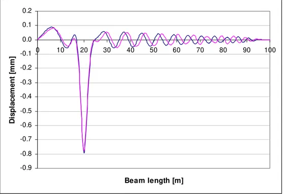
The problem in numerical solution is that with very strong foundation first natural frequencies, ω( )j , are very similar, as it is seen from Equation (8). This can disorder their sequence and consequently attribute different weight to waves forming the transient solution. For instance, by choosing the strong value, 40MN/m2, from Table 1, numerical solution is out of phase further from the load. First of all, there is a significant error in values of natural frequencies, as can be seen in graph in Figure 7. For the sake of comparison, SAP2000 software is included in this comparison. Commercial software gives values lower than analytical ones. Actually, in ANSYS case, error from analytical value is the same for soft and strong foundation, but in the case of strong foundation, vibration modes are disordered to 5,4,6,3,2,7,1,8,9,…, meaning that the lower natural frequency has the 5th mode of vibration, and so on. In Figure 8, displacement in Case study 2 for load at 20m is shown. Out of phase feature is clearly seen. This fact complicates further verifications.
-0.9 -0.8 -0.7 -0.6 -0.5 -0.4 -0.3 -0.2 -0.1 0.0 0.1 0.2
0 10 20 30 40 50 60 70 80 90 100
Beam length [m]
D
isp
lacem
en
t [
m
m
]
Figure 8: Vertical displacement for Case study 2 with v=45.3m/s, no damping and k=40MN/m2, plotted for position of the moving test load at 20m.
(violet curve: analytical solution; blue curve: numerical results)
Here parameter EI k 0.0114
L L
c 1/2
4 4 1
1 =
⎟⎟ ⎠ ⎞ ⎜⎜
⎝ ⎛
μ + μ λ λ = ξ
−
shows sub-critical case, therefore maximum displacement approximately corresponds to steady-state solution:
k 2 P
wmax = β, where 4
EI 4
k
=
Numerical calculation in ANSYS took a significant time, but calculation in Matlab was almost instantaneous, even for very large number of members of sine series. Actually in this case it was necessary to use 90 series to get good approximation (within 0.1%) to the convergence value reached with an exaggerated number of series.
3 Sudden change of vertical stiffness
3.1 Analytical
solution
In order to study sudden elastic foundation stiffness change, implemented in whole region, cantilever dynamic response must be expressed for non-homogeneous static boundary conditions. Then the image of Laplace-Carson transformation,W
( )
j,t , should be modified to:( )
( )
(
( )( )
(
)
)
( )
( )
(
)
(
)
∫
τ − τ −τ τ= t − −τ
0
j t
a j
j
d t b sin e
, L , 0 z EI v Pw b
1 t , j
W . (19)
where
(
)
( )
( )( )
( )
( )( )
(
)
( )
( )( )
( )
( )( )
0 x j j
L x j j
dx x dw EI
t , 0 M 0 w EI
t , 0 V t , L , 0 z
, dx
x dw EI
t , L M L w EI
t , L V t
, L , 0 z
= =
− =
+ −
=
(20)
for left and right clamping, respectively.
( )
( ) ( )( )
( ) ( )(
)
(
)
( )
( )( )
( )
( )( )
( )(
( )(
)
)
( ) ( )( )
( ) ( )(
)
(
)
( )( )
( )( )
( )
( )( )
( ) ( )(
)
(
)
( ) ( )( )
( ) ( )(
)
(
)
( ) ( )( )
( )
( ) ( )(
)
(
)
( ) ( )( )
( )
( ) ( )(
)
(
)
( ) (
)
( )
( ) ( )( )
( ) ( )(
)
(
)
(
)
( )
( ) ( )( )
( ) ( )(
)
(
)
∫
∫
∑
∫
∑
∫
∫
∑
∫
∫
∫
∫
+ + + + + τ τ − − − − τ τ − + − + = τ τ − − τ τ − + τ τ − τ = τ τ − ⎟ ⎟ ⎠ ⎞ ⎜ ⎜ ⎝ ⎛ − + τ τ − τ = ⎟ ⎟ ⎠ ⎞ ⎜ ⎜ ⎝ ⎛ τ τ − ⎟ ⎟ ⎠ ⎞ ⎜ ⎜ ⎝ ⎛ τ − τ + τ τ − τ = τ − − = τ − − = τ − − = = τ − − τ − − = τ − − = τ − − τ − − = τ − − 1 k k 1 k k 1 s s 1 s s 1 s s t t j t a L x j j t t j t a j j k 0 s t t j t a L x j j k 0 s t t j t a j j t 0 j t a j j k 0 s t t j t a L x j j j t 0 j t a j j t 0 j t a L x j j t 0 j t a j j d t b sin e dx x dw b k M 1 k , j M~ d t b sin e L w b k V 1 k , j V~ k , j P ~ d t b sin e s M dx x dw b 1 d t b sin e s V L w b 1 d t b sin e v w b P d t b sin e dx x dw s M L w s V b 1 d t b sin e v w b P d t b sin e dx x dw , L M L w , L V d t b sin e v Pw b 1 t , j WThe only difference is in b ( )j
( )
(
)
( )
( ) ( )( )
( ) ( )(
)
(
)
(
)
( )
( ) ( )( )
( ) ( )(
)
(
)
∫
∫
+ −τ τ− − − + −τ τ+ − = τ − − = τ −
− k1
k 1 k k t t L j t a L x j L j L t t L j t a j R j
L e sin b t d
dx x dw b k M 1 k , j M~ d t b sin e L w b k V 1 k , j V~ t , j W
For the right hand side, however, reversed coordinate can be used
( )
(
)
( )
( ) ( )( )
( ) ( )(
)
(
)
(
)
( )
( ) ( )( )
( ) ( )(
)
(
)
∫
∫
+ −τ τ+ − + + −τ τ+ − = τ − − = τ −
− k1
k 1 k k t t R j t a L x j R j R t t R j t a j R j
R e sin b t d
dx x dw b k M 1 k , j M~ d t b sin e L w b k V 1 k , j V~ t , j W
where internal forces at the discontinuity, V
( )
s and M( )
s , are constant within1 s s;t
t + , 0t0 = and tk+1 =t. For the sake of simplicity it is assumed that the interval 0;t is divided uniformly into k divisions.
Now two cantilever solutions, corresponding to beams clamped on left and right hand side, with different value of Winkler constant can be connected together by continuity conditions. The point of Winkler constant discontinuity corresponds to the point of beam continuity, therefore equilibrium of internal forces must be preserved and equality of vertical displacement and of its spatial derivative (rotation) must be maintained at that point. The internal forces (the unknowns) can be simply introduced by same values in both clamped beam solutions and solved from the equations imposing continuity of vertical displacement and rotation at the point of Winkler constant discontinuity.
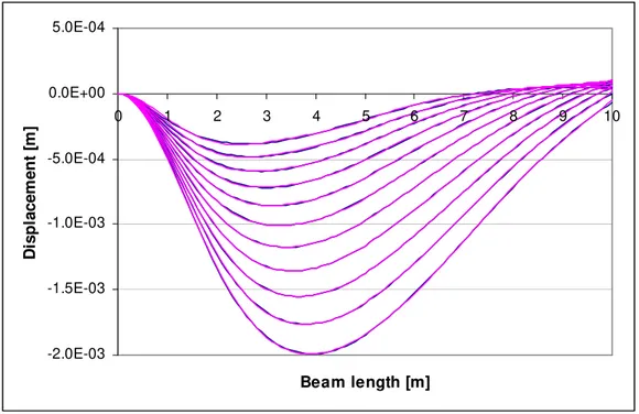
First of all, correctness of this procedure was tested in the opposite way. Clamped beam of L=20m was solved numerically in ANSYS, for the sake of simplicity without elastic foundation and damping and internal forces from its middle section were extracted at each time step. Their linear variation was assumed within each time step. Unfortunately none of the previous integrations could be used in the next time step, due to the convolution form of the integral. Time step divisions were done very fine, 100 steps in each 1m passed by the moving force. Then, deflection curves were completely rebuilt. In the first half of the time needed for the load to cross the structure, the left cantilever solution accounted for the moving load and prescribed internal forces variation at the “free” end. The right cantilever was loaded during this period only by prescribed internal forces variation. Then, when the force passed the middle section, solutions switched their role. Coincidence of results is again very good, as can be seen from Figures 9-10, where left hand side is shown for load position at 0.1, 0.2,…, 1m and results on the right hand side for positions of the load at 1, 1.1, 1.2, …, 2m. Between each pair of curves there are thus 10 time steps involved.
-2.0E-03 -1.5E-03 -1.0E-03 -5.0E-04 0.0E+00 5.0E-04
0 1 2 3 4 5 6 7 8 9 10
Beam length [m]
D
is
p
la
c
e
me
n
t [
m
]
Figure 9: Vertical displacement of the left hand side of the beam plotted for 11 positions of the moving load from 1 to 2m (violet curve: analytical solution; blue
curve: numerical results).
to compare the results with the known analytical solution. Case study 1 was chosen for this purpose, but only force of 10N moving on speed 1m/s was imposed. Internal forces reflected very good coincidence even for 8 series involved, in Figures 11-12 results corresponding to 20 series are shown.
-2.E-05 -5.E-06 5.E-06 2.E-05 3.E-05 4.E-05
10 11 12 13 14 15 16 17 18 19 20
Beam length [m]
D
isp
lace
m
en
t [
m
]
Figure 10: Vertical displacement of the right hand side of the beam plotted for 10 positions of the moving load from 0 to 1m (violet curve: analytical solution; blue
curve: numerical results).
-6 -5 -4 -3 -2 -1 0 1
0 2 4 6 8 10
Time [s]
T
ran
s
ver
sal
f
o
rce [
N
Figure 11: Transversal force distribution in the middle of the clamped beam (violet curve: full analytical solution; blue curve: analytical solution from separate parts for
time steps 0.5s and 0.25s, respectively).
-5 0 5 10 15 20 25
0 2 4 6 8 10
Time [s]
B
e
ndi
ng m
om
e
nt
[
N
m
]
Figure 12: Bending moment distribution in the middle of the clamped beam (violet curve: full analytical solution; blue curve: analytical solution from separate
parts for time steps 0.5s and 0.25s, respectively).
3.2 Parametric analysis in ANSYS
Case study 2 was chosen for further analysis first. Higher value of reference elastic foundation stiffness was chosen in the first half of the structure, 10 times increase in the second half. Total length of 200m was traversed by the reference load with the velocity of 314km/h. Displacements and accelerations are plotted in the region of the stiffness change. They are shown in Figures 13-14. Similar analysis was done in Case study 1, however only twice increase was tested. Accelerations are plotted in the region of the stiffness change in Figures 15.
-4 -3 -2 -1 0 1 2 3 4 5
90 92 94 96 98 100 102 104 106 108 110
Beam length [m]
A
c
cel
er
at
io
n
[
m
/s2]
Figure 13: Accelerations in the location of stiffness increase in Case study 2. (green curve: before; red curve: on the top; blue curve: after the 10 times increase).
-0.5 -0.4 -0.3 -0.2 -0.1 0.0 0.1
90 92 94 96 98 100 102 104 106 108 110
Beam length [m]
D
is
p
la
cem
en
t [
m
m
]
-800 -600 -400 -200 0 200 400 600
90 92 94 96 98 100 102 104 106 108 110
Beam length [m]
Acc
e
le
ra
ti
o
n
[m
/s
2]
Figure 15: Accelerations in the location of stiffness increase in Case study 1. (green curve: before; red curve: on the top; blue curve: after the twice increase).
-1500 -1000 -500 0 500 1000 1500
8 9 10 11 12
Beam length [m]
A
c
cel
er
at
io
n
[
m
/s
2]
Figure 16: Accelerations in the location of stiffness decrease by 5 and 1000000 times in Case study 1.
4 Conclusion
In this paper, analytical transient solutions of dynamic response of one-dimensional systems with sudden change of foundation stiffness are derived. Abrupt localised increase/decrease in foundation stiffness, valid in whole region is solved exactly. However, assumptions about time variation of internal forces at the section of discontinuity had to be adopted and therefore the analytical solution includes numerical procedure. Results are expressed in terms of vertical displacement. Although related to one-dimensional case, this study can give first insight into the problem of excessive ground vibrations induced by high speed trains in regions with vertical stiffness abrupt change.
In these preliminary developments only moving constant force is implemented, therefore structure response is not always in accordance with what is experienced by real rail vehicles. The reason is that the interaction of spring-mass-damper system of the vehicle with the track structure cannot be omitted. This is subject for further research.
References
[1] A. Lundqvist, T. Dahlberg, “Railway track stiffness variations – consequences and countermeasures”, in “Proceedings of the nineteeth IAVSD Symposium on Dynamics of Vehicles on Roads and on Tracks, Milan, Italy, 2005.
[2] H.H. Hung, Y.B. Yang, “A review of researches on ground-borne vibrations with emphasis on those induced by trains”, in “Proceedings of the National Science Council”, Republic of China, Volume 25, Number 1, 1-16, 2001. [3] H. Lamb, “On the propagation of tremors over the surface of an elastic
solid”, Philosophical Transactions of the Royal Society A, Volume 203, 1-42, 1904.
[4] S.P. Timoshenko, “Statical and dynamical stresses in rails”, in “Proceedings of the International Congress of Applied Mechanics”, Zurich, Switzerland, 407-418, 1926.
[5] L. Frýba, “Vibration of solids and structures under moving loads”, Third Edition. Thomas Telford, 1999.
[6] M. Shamalta, A.V. Metrikine, “Analytical study of the dynamic response of an embedded railway track to a moving load”, Archive of Applied Mechanics, 73, 131-146, 2003.
[7] A.V. Metrikine, K. Popp, “Vibration of a periodically supported beam on an elastic half-space”, European Journal of Mechanics, A/Solids, 18, 679-701, 1999.
[9] A.V. Vostroukhov, A.V. Metrikine, “Periodically supported beam on visco-elastic layer as a model for dynamic analysis of a high-speed railway track”, International Journal of Solids and Structures”, 40, 5723-5752, 2003.
[10] X. Sheng et. al., “Ground vibration generated by a load moving along a railway track”, Journal of Sound and Vibration, 228(1), 129-156, 1999.
[11] G. Lombaert, G. Degrande, D. Clouteau, “The influence of the soil stratification on free field traffic-induced vibrations”, Archive of Applied Mechanics, 71, 661-678, 2001.
[12] P. van den Broeck, G. Degrande, G. de Roeck, “A prediction model for ground-borne vibrations due to railway traffic”, in “Proceedings of the Fifth European Conference on Structural Dynamics, EURODYN’2002”, Munich, Germany, 503-508. 2002.
[13] N.A. Haskell, “The Dispersion of Surface Waves on Multilayered Media”. Bulletin of the Seismological Society of America, 43, 17-34, 1953.
[14] E. Kausel, J.M. Roësset, “Stiffness Matrices for Layered Soils”, Bulletin of the Seismological Society of America, 71(6), 1743-1761, 1981.
[15] A.M. Kaynia, C. Madshus, P. Zackrisson, “Ground Vibration from High-Speed Trains: Prediction and Countermeasure”, Journal of Geotechnical and Geoenvironmental Engineering, 126, 531-537, 2000.
[16] Release 14 Documentation for MATLAB, The MathWorks, Inc., 2004.
[17] Release 10.0 Documentation for ANSYS, Swanson Analysis Systems IP, Inc., 2006.
[18] G. Degrande, L. Schillemans, “Free Field Vibrations during the Passage of a Thalys High-Speed Train at Variable Speed”, Journal of Sound and Vibration 247(1), 131-144, 2001.