Published online 3 June 2016 in Wiley Online Library (wileyonlinelibrary.com). DOI: 10.1002/cpe.3860
A high-performance computing framework for Monte Carlo
ocean color simulations
Tamito Kajiyama
1, Davide D’Alimonte
1and José C. Cunha
21CIMA, Universidade do Algarve, Campus de Gambelas, Faro 8005–139, Portugal
2NOVA LINCS, DI/FCT, Universidade Nova de Lisboa, Quinta da Torre, Caparica 2829–516, Portugal
SUMMARY
This paper presents a high-performance computing (HPC) framework for Monte Carlo (MC) simulations in the ocean color (OC) application domain. The objective is to optimize a parallel MC radiative transfer code named MOX, developed by the authors to create a virtual marine environment for investigating the quality of OC data products derived fromin situmeasurements of in-water radiometric quantities. A consolidated set of solutions for performance modeling, prediction, and optimization is implemented to enhance the efficiency of MC OC simulations on HPC run-time infrastructures. HPC, machine learning, and adaptive computing techniques are applied taking into account a clear separation and systematic treatment of accuracy and pre-cision requirements for large-scale MC OC simulations. The added value of the work is the integration of computational methods and tools for MC OC simulations in the form of an HPC-oriented problem-solving environment specifically tailored to investigate data acquisition and reduction methods for OC field mea-surements. Study results highlight the benefit of close collaboration between HPC and application domain researchers to improve the efficiency and flexibility of computer simulations in the marine optics application domain. © 2016 The Authors.Concurrency and Computation: Practice and ExperiencePublished by John Wiley & Sons Ltd.
Received 21 September 2013; Revised 22 January 2016; Accepted 17 April 2016
KEY WORDS: high-performance computing; Monte Carlo simulation; ocean color; uncertainty
1. INTRODUCTION
Research at the interface of Geosciences and Computer Science increasingly demands large-scale high-performance computing (HPC) applications. Simulation-driven experimentation in Geo-sciences generally involves complex mathematical models and large volumes of data. HPC solutions tailored to specific application areas can help improve the quality of numerical results through a comprehensive exploitation of computational resources. Scientific studies relying on HPC facilities need to meet different performance and efficiency requirements including the following: (1) opti-mization of time and space costs for running large-scale computer simulations; (2) comprehensive exploitation of consolidated and emerging computer architectures in different geographical settings; and (3) ease of access to computing resources and supporting HPC techniques. These requirements have been the rationale of numerous HPC applications in Geosciences (e.g., [1–6]), stimulating a variety of Computer Science studies on HPC-oriented problem-solving environments (PSE). Key PSE components include parallel and grid computing infrastructures [7, 8], middleware and programming tools [9–12], and computational methods for Geoscience applications [13–16].
Within the scope of the Geo-Info project [17] aiming to promote joint research between com-puter scientists and Geoscience experts, this paper presents an HPC framework for performance prediction and optimization of Monte Carlo (MC) simulations for ocean color (OC) applications.
*Correspondence to: Tamito Kajiyama, CIMA, Universidade do Algarve, Campus de Gambelas, Faro 8005–139, Portugal.
†E-mail: [email protected]
Figure 1. Study components with specific uncertainty budgets.
This framework concerns a parallel MC radiative transfer code [17–20], hereafter referred to as MOX, developed by the authors to support investigations on OC data products derived fromin situ
radiometric measurements perturbed by uncertainties due to environmental factors [21–23]. The MOX implementation is underpinned by the increasing importance of accurate long-termin situOC measurements for the development of bio-optical models, vicarious calibration of satellite sensors, and validation of remote sensing (RS) radiometric products [24–30]. Earth observation programs of relevance include the MERIS and OLCI projects of the European Space Agency and the Sea-WiFS, MODIS, and VIIRS projects of the US National Aeronautics and Space Administration. MOX computes the light distribution in natural waters by tracing a number of photons and track-ing their trajectories. The output of the photon tractrack-ing is a two-dimensional virtual representation of in-water radiometric fields, which can then be used as a controlled environment to derive OC data products with statistical features analogous to those in reality. MOX can hence contribute to theoret-ical assessments of uncertainty budgets in OC field measurements and provide guidelines to refine data reduction methods forin situmarine radiometry [31–33].
An integrated set of HPC techniques for MOX performance prediction and optimization is imple-mented in this study to enhance the efficiency of MC OC simulations on large-scale parallel computers. This objective is challenged by heterogeneous uncertainty characterizing OC applica-tions, MC simulaapplica-tions, and HPC systems. These uncertainty budgets, hereafter respectively referred to as OC, MC, and HPC uncertainty, are addressed in a component-wise manner (Figure 1). The OC uncertainty represents perturbations affecting the quality of OC data products, specifically the following: (1) the precision (i.e., reproducibility) ofin situmeasurements and (2) the accuracy of RS observations with respect to referencein situdata. The former refers to those perturbations due to environmental conditions and measurement settings that MOX is intended to analyze. The latter uncertainty is a matter of satellite OC investigations, which set up the encompassing context of the present work. The MC precision accounts for statistical fluctuations intrinsic to the randomness of MC methods [34–36] affecting the reproducibility of simulation results. The MC accuracy deter-mines the physical correctness of simulated radiometric fields [18]. The HPC uncertainty finally refers to performance variability observed in parallel computing systems [37–40]. This variability influences the precision of execution time assessments based on which performance prediction is attempted, and hence also the accuracy of prediction results with respect to reference execution time. Large-scale MOX simulations are motivated by (1) the necessity to satisfy MC precision require-ments and (2) the need to explore various environmental cases of interest in OC investigations. Specifically, the present HPC framework aims to address two goals:
(2) Efficient exploitation of HPC systems. MOX is used by domain experts to explore a wide multi-dimensional parameter space defined by case study specifications. This may require hun-dreds of simulation jobs. It is hence desirable to distribute the simulation jobs to the available computing environments in a cost-effective manner based on an automated job scheduling mechanism. The foremost objective of job scheduling is to minimize time costs because of expensive computation time in HPC facilities. The job-environment mapping can be auto-mated by means of execution time estimates. However, predictive performance modeling of the MOX code is challenged by the aforementioned issue of photon population size, as well as by a nonlinear dependence of the execution time upon multivariate simulation settings, includ-ing illumination conditions, seawater optical properties, and irregular boundary conditions imposed by sea-surface waves (e.g., [18]).
The main achievements of the present work are summarized hereafter:
(1) From a Computer Science perspective, this study makes a case of an effective combination of HPC, machine learning, and adaptive computing techniques to address the performance prediction and optimization problems posed by large-scale MC simulations in the presence of OC, MC, and HPC uncertainty budgets.
(2) From an applicative point of view, instead, it provides OC scientists with a suite of compu-tational methods that improve the efficiency and flexibility of MOX experiments, benefiting application case studies conducted on supercomputers.
1.1. Related work
The present work advances reference research achievements [19, 20] by integrating new results and methods in a unifying framework of performance optimization techniques. Numerical results acknowledge an extended range of input simulation parameters to investigate the effects of envi-ronmental factors on run-time performance optimization. Besides, the offline performance tuning scheme outlined in [20], here revised from a methodological perspective, is evaluated based on novel numerical results. The study is part of a wide range of performance modeling solutions for optimizing time and space in simulation-driven investigations for Geosciences, as reviewed next.
Performance modeling and prediction in the literature can be roughly divided into three classes:
Fully analytical modeling based on in-depth knowledge of target computer programs and envi-ronments [41–43]; semi-analytical modeling based on a priori knowledge of the programs and environments to identify appropriate model expressions, and least-squares fitting of model coef-ficients to observed performance data [44–50]; and empirical performance modeling relying on very general model expressions whose coefficients are learned from data [48, 51]. The key element exploited for MOX performance modeling is the identification of linear and nonlinear components in the photon tracing time. The linear dependence is treated analytically, while an empirical multi-layer perceptron (MLP) scheme is used to model the nonlinear relationship.
MLP neural networks have been widely used for a number of applications including perfor-mance modeling [48, 51], job scheduling [52], load balancing [53], design space exploration [54, 55], and OC bio-optical inversion [29, 30, 56–64]. A common finding among these studies is that a key to successful MLP applications is empirical tuning of MLP algorithms in terms of network architecture, data pre-processing, and application-specific feature selection. Developing MLP algo-rithms usually requires a thorough adaptation of the generic neural computing framework to specific application cases.
Adaptive computing applications commonly exploit domain-specific elements in order to enable automated dynamic optimization. The online accuracy evaluation scheme applied in this study is an example of a widely used procedure where computation continues (either iteratively or recursively) until predefined accuracy conditions are met. Many other examples of domain-specific adaptive computing techniques are found in the literature, for instance in self-adapting linear algebra [67–69], adaptive quadrature [70, 71], and adaptive mesh refinement [42, 72] just to name a few. These previous studies and the present work differ in the ways how domain-specific elements are used to control adaptive iteration/recursion procedures.
Our adaptive performance tuning shares strategies with the adaptive control theory [73]. In both cases, the objective is the adaptive scheduling of computations upon run-time events. Canonical control theory relies on formal expressions through an analytical (e.g., [74]) or a machine learning approach (e.g., [75]) to model the distribution of the system state. In the present study, decision making does not require learning the occurrence of different events (hence there is no need for probability density estimation). Instead, adaptive strategies are decided on prior knowledge of run-time events.
1.2. Structure of the work
The paper organization is as follows. Section 2 presents a general architecture of HPC-oriented problem-solving environments based on which the present work is developed. Section 3 examines MOX performance characteristics. On this analysis basis, the components of the proposed HPC framework are formulated in Section 4. The system components are then verified by experimental results in Section 5 and further discussed in Section 6. Finally, Section 7 concludes the work with a summary of the study and elements for future progresses.
2. HPC-ORIENTED PROBLEM-SOLVING ENVIRONMENTS
Scientific and engineering applications increasingly rely on virtual experiments by means of numerical simulations to better understand the behavior of real complex systems under different con-figuration scenarios. The growing demand of a systematic support for simulation-based experiments has pushed forward the development of integrated solutions commonly called PSEs. This concept, appeared in the 1990s [76], is now a recognized approach to help scientists and engineers manage the complexity of problem solving. The scope is to provide a transparent and easy-to-use interface to state-of-the-art algorithms and problem-solving strategies. Large-scale and data-intensive applica-tions as those addressed here require dedicated support and easy access to underlying run-time HPC systems, as well as efficient and scalable means for job and resource management, data visualization and analysis.
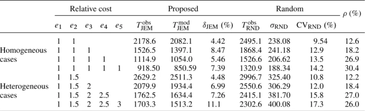
The schematic in Figure 2 identifies the following four main PSE functional layers for HPC applications.
(1) Application set-up. This layer accommodates domain-specific abstractions, mathematical models and solvers, as well as experiment scenarios in terms of parameters and objective func-tions for optimization. In the present study, this layer includes the MOX code and case study specifications.
(2) Experiment management. This layer comprises generic components for managing the problem-solving process, that is,
(a) Experiment specification, which allows users to describe structural or template plans for computer experiments.
(b) Design space exploration, optimization, and tuning, based on a set of design alterna-tives corresponding to various configurations of input parameters.
Figure 2. Architectural overview of problem-solving environments (PSEs). Rectangles represent general PSE components, whereas rounded boxes highlight study elements of the present work.
performance enhancement of MOX simulations through online accuracy evaluation and offline threshold parameter tuning.
(3) Job and resource management.This layer offers functionalities to automate the instantiation of simulation jobs and management of their execution in underlying run-time infrastructures. In the case of the present work, this layer includes techniques for predictive performance modeling and job scheduling on the basis of past MOX execution records.
(4) Computing infrastructure. This layer represents execution platforms for HPC applications including clusters, grids, and clouds. The target computing environments of this work are distributed-memory and shared-memory parallel machines.
3. MOX PERFORMANCE CHARACTERIZATION
This section addresses the performance characterization of the MOX code. MOX features relevant to this study are also presented for convenience of the readers (see [18] for more detail).
MOX applications start with MC simulations of in-water radiometric fields, followed by ‘virtual’ optical profiling where the simulated radiometric fields are used to derive data products relevant for OC studies.
MC simulations constitute the most compute-intensive part of MOX applications. The simulation domain is anx–´cross section of a seawater column (from surface to bottom) modeled as vertically stacked layers of horizontal photon-collecting bins (Figure 3). The output of photon tracing provides the spatial distributions of different radiometric quantities<k.k D 1; 2; 3; : : :/. Each radiometric field, expressed by a matrix whose.i; j /entry accumulates photons that hit thej-th bin of thei -th layer, is -then used for virtual optical profiling complying wi-th measurement protocols ofin situ
marine optics.
Figure 3. Schematic of MOX simulation domain and photon trajectory.
Figure 4. Panel (a) shows a simulated radiometric field (referred to as downward irradianceEd [18]) in the presence of sea-surface waves. Spatial variability of the light distribution in the water illustrates the light focusing and defocusing effects induced by the sea surface. White diagonal lines indicate a virtual deployment path of a profiler system below the sea surface (in-air trajectories in red are not considered for data sampling). Panel (b) shows a set ofEd.ı´/values (circles) sampled at different depthsı´ along the
(circles) sampled at different depthsı´along the deployment path in the radiometric field. A data reduction method is then applied to these sampled values to compute the radiometric data products of interest.
Only the MC computation has been parallelized, because the time spent for virtual optical profiling is negligible with respect to the photon tracing time.
3.1. Parallelization
MC radiative transfer simulations belong to the class of embarrassingly parallel problems, where each photon transport can be computed independently of the others. MOX exploits data parallelism through full replication of radiometric field matrices as follows. The total number of photons Np is evenly divided intoNcCPU cores. Each CPU core computes the trajectories ofNppc D Np=Nc photons using a different random number seed. For each radiometric quantity, matrices on theNc CPU cores are gathered and summed up at the end of the simulation. This summation is carried out by a parallel reduction operation, which involvesNc1matrix additions.
Two versions of the parallel MOX code were implemented, one with MPI for distributed-memory parallel computers and the other with OpenMP for shared-memory machines. Both implementations show similar parallel performance because of the embarrassingly parallel workload. This paper focuses on the MPI version of the code, since it enables numerical experiments with a larger number of CPU cores.
3.2. Execution time components
The execution time of the parallel MOX code consists of three components: initialization, photon tracing, and matrix summations. The initialization time, spent for reading a simulation configu-ration file and preparing zero-filled radiometric field matrices, is negligible. The photon tracing time is dominant (more than 99 %) when considering the number of photons per CPU core (106or larger) typically required for application studies. The time spent for matrix summations can also be neglected with respect to the photon tracing time. Only the photon tracing time is henceforth referred to as the execution time of MOX.
The photon tracing time may vary significantly depending on various input simulation parame-ters, including the seawater IOPs (i.e., attenuation and absorption coefficients, and volume scattering function), illumination conditions (i.e., the sun position, sky radiance distribution, and diffuse-to-total irradiance ratio), sea-surface geometry (expressed by the lengths and heights of harmonic waves), dimensions and spatial resolution of the simulation domain, and photon weight threshold. Clearly, the photon tracing time also depends on performance factors of execution environments such as CPU clock frequency, memory bandwidth, and memory latency.
3.3. Parallel performance and uncertainty
This section describes MOX performance characteristics through experiments using the Milipeia cluster (University of Coimbra, Portugal). The cluster consists of identical compute nodes on a Giga-bit Ethernet interconnect. Each node has two dual-core AMD Opteron 275 processors at 2.2 GHz and 8 GB RAM.
Table I shows photon tracing timeT (in seconds; averaged over five samples) as a function of Nppcin the case ofNcD4andNppcset equal to a power of 10. The ratior DT .Nppc/=T .Nppc=10/ is approximately 10 whenNppc>105, which indicates thatT is proportional toNppcin operational MOX applications.
Table I. Photon tracing timeT (in seconds; averaged over five samples) on Milipeia as a function ofNppc in the case ofNc D4andNppcset equal to a power
of 10.
Nc Np Nppc T r
4 4101 101 1:98410 1 — 4 4102 102 3:17210 1 1.599 4 4103 103 1:284100 4.048 4 4104 104 1:036101 8.07 4 4105 105 1:011102 9.752 4 4106 106 9:988102 9.884 4 4107 107 1:007104 10.08
Ratio r D T .Nppc/=T .Nppc=10/is approximately 10
whenNppc > 105, indicating thatT is proportional to Nppc.
Table II. Maximum, mean, standard deviation, and coefficient of vari-ation (Tmax; ; , and CV, respectively; averaged over five samples) of per-core photon tracing timeTi (in seconds) on Milipeia as a function of
Ncin the case ofNppc D2106, where subscripti is a serial CPU core number (i D1; 2; : : : ; Nc) and CVD100=Œ%.
Nc Np Nppc Tmax CV
4 8106 2106 1974.5 1947.9 36.12 1.85 %
8 16106 2106 2004.7 1962.3 33.19 1.69 %
16 32106 2106 2004.6 1952.9 32.59 1.67 % 32 64106 2106 2006.6 1949.8 39.18 2.01 % 64 128106 2106 2057.3 1970.5 42.33 2.15 % 128 256106 2106 2090.4 1975.1 42.42 2.15 %
Average — — — 1968.4 42.17 2.14 %
CV, coefficient of variation.
Figure 5. Distribution of observed per-core photon tracing timeTiin the case ofNcD128in Table II.
Figure 6. Comparison of measured maximum photon tracing time Tmax with theoretical results. The cir-cles are the measuredTmaxvalues (Table II) normalized by z-score transformation.Tmax/=, where and are the mean and standard deviation of measuredTi values, respectively. The solid line, based on
Eq. (9) in [78], shows the theoretical expected maximum value amongNc independent and identically dis-tributed samples drawn from a normal distribution with zero mean and one standard deviation,N.0; 1/. The pluses and crosses show two sets of expected maxima determined by Monte Carlo (MC) simulations [78]
with 1000 and 5 trials, respectively.
In summary, the MOX parallel performance is quantified by the maximum per-core photon trac-ing time, which is proportional to Nppc (Table I) and weakly depends on Nc (Table II). These characteristics define MOX performance modeling and job scheduling methods (Sections 4.1 and 4.2).
3.4. Performance tuning
Figure 7. Framework components for high-performance MOX simulations.
4. METHODS
This section presents the four components of the HPC framework for large-scale MC OC simu-lations: (1) MLP algorithms for execution time prediction; (2) job-environment mapping (JEM) algorithm; (3) adaptive termination of photon trajectory tracking; and (4) offline optimization of photon weight threshold. The first two components permit an automated job scheduling scheme for large simulation-based experiments in OC application studies, whereas the other two allow for enhancing the MOX performance. Figure 7 shows the interaction of the four components, which are presented in the subsequent sections.
4.1. Hybrid approach for execution time prediction
MOX execution time is predicted jointly using an analytical model and an empirical MLP regression scheme. The rationales of this hybrid approach are the following. First, the MOX execution time is proportional to the number of photons per CPU core and approximately inversely proportional to the number of CPU cores (Section 3.3). These properties are easy to capture by a linear expression. Second, the photon tracing time shows a nonlinear dependence on input simulation parameters, which is analytically intractable. Hence this component is modeled using MLP neural networks (see [19] for more detail).
The expected execution timeT of a production MOX run in a particular parallel computing environment is modeled as a function of a set of input simulation parameters, the number of CPU coresNc, and the number of photonsNpas follows:
(1) A training dataset is built by running a set of simulation jobs and measuring the time spent for tracing a reduced number of photonsNOpseveral orders of magnitude smaller thanNp, and using a limited number of CPU coresNcO < Nc.
(2) An MLP is built from the training dataset and then used for predicting the timeTO to be spent for tracingNOpphotons usingNOcCPU cores based on the given set of input simulation parameters. (3) The predictionT is computed by linear extrapolation as
T DNOc=Nc Np=NOp
O
T : (1)
Figure 8. The job-environment mapping scheme.
4.2. Job-environment mapping algorithm
This section presents the JEM algorithm to minimize the total time for running MOX simulation jobs distributed to multiple execution environments [19]. LetSD ¹s1; : : : ; sN
sºbe a set ofNssimulation jobs,E D ¹e1; : : : ; eN
eºbe a set of Ne execution environments, andfij D f .si; ej/represent the cost of running si on ej. The cost function f is defined by means of MLP algorithms for execution time prediction. Figure 8 shows the JEM scheme. It employs a greedy strategy to assign jobs to environments in descending order of time costs. This mapping algorithm complements the MLP performance prediction, and they provide a complete tool set of HPC job scheduling foreseen in Figure 7.
4.3. Adaptive termination of photon trajectory tracking
The execution time of a MOX simulation job is decoupled into two parts. One is the time employed for computing photon trajectories. The other is the time for tracking the photon trajectories by adding the photon weight into the entries of radiometric field matrices along the photon trajectories. Some matrices are updated, while the others are left unchanged depending on the photon traveling direction and field-of-view angles of radiometers being simulated [18]. For example, the radiometric field shown in Figure 4(a) is computed by accumulating only those photons traveling downwards.
Light in a homogeneous seawater column decreases approximately exponentially with depth ı´ [79]. Indicating with <k radiometric quantities (k D 1; 2; 3; : : :) and omitting the spectral dependence for brevity, the decrease of<kwithı´is expressed as follows:
<k.ı´/D <k.0 /exp.K<k ı´/; (2)
where<k.0 /are subsurface radiometric values just below the sea surface,K<k are diffuse attenu-ation coefficients, andı´is positive downward. In field marine radiometry,<k.0 /andK<k are the OC quantities of interest derived applying a regression scheme to a set of<k.ı´/values measured at different depthsı´in the water column. In MOX application scenarios, simulated radiometric fields are used for virtual optical profiling to evaluate the precision of OC data products under controlled simulation conditions that could not be attained in the natural environment.
With = generically indicating data reduction results [either <k.0 / or K<k of Eq. (2)], the
uncertainty observed in a set of=j values is expressed by the CV in percent defined as
CV=D100 q
1 N
P
j
=j h=i 2
h=i ; (3)
whereNis the number of=j values and
h=i D 1
N
X
j
=j: (4)
MOX simulations concern two general types of environmental conditions hereafter referred to as Types I and II, respectively. Type I simulations are those with an ideal flat sea surface, whereas Type II simulations acknowledge the presence of sea-surface waves. Experimental results with MOX simulations have shown that (1) CV= decreases infinitely with an increasing number of photons
in Type I simulations, and (2) CV= reaches a plateau at a certain number of photons in Type II
simulations [18]. In the Type I simulations, tracing more photons does not significantly improve the reproducibility of OC data products after the MC noise is reduced to an acceptable level. In the Type II simulations, the variability cannot be reduced below a certain level no matter how many extra photons are traced, due to genuine light variability caused by the focusing effects of sea-surface waves. Note that the number of photons necessary to neglect the MC noise is unknown in advance in both cases.
The MOX performance is optimized based on online quality evaluation of radiometric field matri-ces to stop tracking photon trajectories when predefined precision criteria are met [20]. The rationale behind this early termination of photon trajectory tracking is that it is a waste of time and computing resources to keep updating the matrices that are already free of MC-intrinsic statistical noise.
The adaptive termination of photon trajectory tracking is performed as follows. Every time a certain number of photons on different orders of magnitude (e.g., 103,104, and105) have been traced, the statistical quality of radiometric field matrices is quantified by the CV=values of Eq. (3).
Specifically, for each radiometric quantity<kand data product=, the following stopping criteria are tested:
CV=< 0:1 (5)
200 CV
0
=CV=
CV0=CCV=
< 5 (6)
where CV0=refers to the CV=value in the previous evaluation. The first condition imposes a target
precision of 0.1% to take into account that the CV of data reduction results keeps decreasing as photon tracing continues in Type I simulations. The second condition relies on the unbiased percent difference between the present and previous CV values to detect a saturation pattern of CV reduction rate in Type II simulations. The unbiased percent difference threshold is here set to 5%. If one of the stopping criteria is met, then the updates of the<kdata matrix are terminated. Photon tracing is, however, continued until photon trajectory tracking has been stopped for all radiometric quantities of interest.
4.4. Offline optimization of photon weight threshold
perspective. In contrast, thresholding the photon weight is suggested by a cost-effectiveness con-sideration, because a photon weight close to zero does not significantly contribute to the statistical quality of simulated light fields.
A thorough examination of OC and MC application requirements thus permits performance opti-mization based on quality-speed trade-offs. The case considered here is that a smallerwimproves the precision of simulated radiometric fields, whereas a largerwleads to a shorter photon lifetime, which translates into a shorter execution time.
Seawater IOPs and photon weight threshold jointly determine the average depth that photons can reach within the water column. Simulated light fields below this average depth are not be suitable for virtual optical profiling due to increased MC statistical noise. Note also that virtual optical profil-ing is conducted by samplprofil-ing radiometric values within an upper layer of the water column, namely, between just below the surface and a predefined depth referred to as the regression layer depth [31]. Hence the average photon depth must be deeper than the regression layer depth.
The objective is then to determine the largest value ofwso that data reduction results are not affected by MC statistical noise. To this end, the photon weightwis parameterized as a function of the depth´[m] (positive downward) in the seawater medium having attenuationcand absorption acoefficients [m 1]. To simplify this parameterization, an ideal flat surface illuminated only by the sun at the zenith is considered. By the same token, forward scattering is adopted for an analytical approximation of the problem.
The initial photon weight is set to one. Every time the photon is scattered by the seawater, the weight is scaled by single scattering albedo! D.ca/=cto account for absorption by the seawater. Therefore, the number of scattering events mafter which the weight becomes smaller thanwis implicitly expressed as
!mDw: (7)
By solving form,
mDlogw=log!: (8)
This gives the maximum number of scattering events that a photon may undergo before tracing of the photon is terminated. Equation (8) indicates that for a fixed! lower than 1 by definition, an exponential increase ofw(e.g., from10 6to10 3) leads to a linear decrease ofmand thus of the per-photon and total execution time.
The optical distance that a photon travels before a scattering event is given by an exponential probability density function
p. /Dexp. /; (9)
where >0. The expectation value ofisE. /D1. The geometrical distancer[m] is defined as r D=c, so that the photon travelsE.r/D1=con average between scattering events. The average depth´that the photon can reach afternscattering events is at most
´DnE.r/Dn=c; (10)
and hence
nDc´: (11)
The maximum photon weight afternscattering events is finally expressed as a function of´as
wD!c´: (12)
Table III. MOX simulation configurations, with different values for five input parameters: attenuation c and absorption a coefficients [m 1], sun zenith angles[deg.], and surface wave lengthsl and heightsh[m]. Single
scattering albedo!D.ca/=cis additionally shown.
Conf. c a ! s l h
1a 0.2 0.15 0.25 30 5 0.5
1b 0.5 0.05 0.9 30 5 0.5
1c 0.6 0.5 0.17 30 5 0.5
1d 1 0.2 0.8 30 5 0.5
2a 0.2 0.15 0.25 60 5 0.5
2b 0.5 0.05 0.9 60 5 0.5
2c 0.6 0.5 0.17 60 5 0.5
2d 1 0.2 0.8 60 5 0.5
3a 0.2 0.15 0.25 30 5, 0.5 0.5, 0.05
3b 0.5 0.05 0.9 30 5, 0.5 0.5, 0.05
3c 0.6 0.5 0.17 30 5, 0.5 0.5, 0.05
3d 1 0.2 0.8 30 5, 0.5 0.5, 0.05
4a 0.2 0.15 0.25 60 5, 0.5 0.5, 0.05
4b 0.5 0.05 0.9 60 5, 0.5 0.5, 0.05
4c 0.6 0.5 0.17 60 5, 0.5 0.5, 0.05
4d 1 0.2 0.8 60 5, 0.5 0.5, 0.05
5a 0.2 0.15 0.25 30 0 0
5b 0.5 0.05 0.9 30 0 0
5c 0.6 0.5 0.17 30 0 0
5d 1 0.2 0.8 30 0 0
5. RESULTS
Table III shows 20 MOX parameter sets from real case scenarios [18] taking account of five input quantities: seawater attenuationcand absorptiona coefficients [m 1], sun zenith angles [deg.], surface wave length l, and heighth [m]. Four sets of seawater optical property values, two sun elevations, and three sea-surface states are considered. Sea-surface geometry is modeled as the sum of harmonic waves. Attenuation and single scattering albedo indicate that the considered simulations concern various seawater types ranging from clear to turbid waters (c 2 Œ0:2; 1), as well as from less to more scattering waters (!2Œ0:17; 0:9).
5.1. MLP algorithms for execution time prediction
This section concerns the validation of the MLP performance modeling method (Section 4.1). MLPs for predicting the execution time of the 20 simulation configurations in Table III are developed on the basis of execution time measurements collected by running training simulations.
Selected MLP input parameters are attenuationc and absorptionacoefficients and sun zenith angles. To account for different sea-surface states, the 20 test simulation cases were split into three groups W1, W2, and F as shown below, and a separate MLP was trained for each group:
W1 Conf. 1a–1d and 2a–2d with one wave component. W2 Conf. 3a–3d and 4a–4d with two wave components. F Conf. 5a–5d with flat surface.
combines each of fiveavalues at log-scale regular intervals with threecvalues betweenaandamax at linear uniform intervals, whereamaxwas set equal to 1.1. In all cases, a total of 15 pairs ofcand avalues as well as the same set of threes values (i.e., 20, 45, and 70 degrees) were used, so that each training dataset includes 45 samples.
MLP training and validation were repeatedM D 10 times to assess the average MLP perfor-mance taking account of variations in prediction results due to the nonlinear optimization performed to train the MLP. The relative prediction error in percent is defined as
ki D100y k i ti
ti
; (13)
wheretidenotes the observed execution time of thei-th simulation configuration andyikis the cor-responding execution time prediction from thek-th MLP. The average MLP performance is assessed by the mean and standard deviationofikvalues computed overN simulation configurations andMpredictions for each configuration:
D 1 M 1 N M X
kD1 N
X
iD1
ik; (14)
D 1 M 1 N M X
kD1 N
X
iD1
ik
2 !1=2
: (15)
Figure 9 shows MLP prediction results in the right column panels. Circles (blue), triangles (green), and squares (red) indicate results for Groups W1, W2, and F, respectively. The markers show the mean ofMexecution time predictions, with error bars indicating˙1standard deviation. The MLPs trained with the dataset in Panel 9(a) gave smallervalues but larger prediction uncer-tainties, especially at longer execution time. This is likely explained as an extrapolation problem due to the training data that do not completely cover the parameter space including the validation cases. The training data in Panel 9(c) represent a more regular sampling but also an uneven distribu-tion with respect to the validadistribu-tion samples. This may explain the large predicdistribu-tion errors due to MLP learning with sparse training data. The most performing MLPs (i.e., with a moderate and the smalleston average) were those trained with the dataset in Panel 9(e). This case study highlights the importance of a careful selection of training samples to avoid MLP extrapolation and learning from sparse data.
5.2. Job-environment mapping algorithm
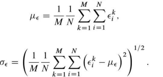
The relevance of the proposed JEM algorithm is evaluated by considering the scheduling perfor-mance of random job allocation (RND) as benchmark. When no prior information is available about the execution time of individual MOX simulations, the most general scheduling approach is ran-dom allocation assuming the same running cost for all jobs (homogeneous cases). If relative running costs of different computing environments are known, then more jobs can be assigned to less costly computing environments (heterogeneous cases). These two scheduling scenarios are used for eval-uation, considering as a case study the problem of allocating the 20 simulation jobs of Table III to a different number of computing environments ranging from 2 to 5. Results are presented in Table IV through the quantities defined hereafter.
The columns labeledei(i D1; : : : ; 5) indicate relative costs for running jobs in the five comput-ing environments (blank entries mean unused). Concerncomput-ing the JEM approach matter of this study, MLP performance models are trained adopting the dataset of Figure 9(e). The 20 jobs are then allo-cated to multiple environments based on MLP execution time estimates, and for each environment, the total execution time of allocated jobs are calculated.Tobs
JEMindicates the observed maximum total execution time (in seconds) among the computing environments, while Tmod
JEM corresponds to the modeled execution time. The relative percent difference between observed and modeled values is ıJEMD100
Tmod JEM TJEMobs
=Tobs
Figure 9. Panels (a), (c), and (e) in the left column show three data distributions, with blue dots and red crosses indicating training and validation samples, respectively. Note that the distributions of validation values are the same for all tested cases. Panels (b), (d), and (f) in the right column indicate validation results of the multi-layer perceptron (MLP) execution time models built with training samples in the corresponding left column panels. MLP performance is assessed by mean relative error and standard deviation
(shown in the form˙) computed for all the 20 validation cases (indicated as ‘overall’), as well as for
Table IV. Performance analysis of scheduling algorithms. MOX execution times are expressed in seconds (see text for detail).
Relative cost Proposed Random
(%) e1 e2 e3 e4 e5 Tobs
JEM TJEMmod ıJEM.%/ TRNDobs RND CVRND.%/
1 1 2178.6 2082.1 4.42 2495.1 238.08 9.54 12.6
Homogeneous 1 1 1 1526.5 1397.1 8.47 1868.4 241.18 12.9 18.2
cases 1 1 1 1 1114.9 1054.0 5.46 1526.6 206.62 13.5 26.9
1 1 1 1 1 918.50 850.59 7.39 1320.9 188.34 14.2 30.4
1 1.5 2629.2 2511.3 4.48 2996.7 325.40 10.8 12.2
Heterogeneous 1 1.5 2 2079.9 1934.4 6.99 2550.6 306.29 12.0 18.4
cases 1 1.5 2 2.5 1762.5 1634.4 7.26 2415.1 381.70 15.8 27.0
1 1.5 2 2.5 3 1703.3 1513.2 11.1 2302.6 400.08 17.3 26.0
time observed upon 10000 random job allocations. By the same token,RNDand CVRND are the standard deviation and the CV, respectively. Finally,D100.Tobs
JEMTRNDobs/=TRNDobs reports relative performance gains by the JEM method with respect to the benchmark results.
In homogeneous cases, relative costsej were set to 1 for all environments, and only the number of available computing systems was changed. In the case of two environmentse1ande2, for example, the JEM algorithm allocated 9 and 11 jobs toe1ande2, respectively. The observed (modeled) total execution time ine1 ande2 was 2178.6 (2082.1) and 2151.9 (2080.0) seconds, respectively. With the RND scheme, the 20 jobs were evenly assigned to the two environments at random. The result isTobs
RNDD2495:1, which corresponds to a gain ofD12:6%.
In heterogeneous cases, relative differences in job execution costs were modeled by a linear scal-ing factor indicated as ei in the table. Both the observed and modeled execution times of the 20 MOX simulation jobs were scaled byeito account for heterogeneous performance of the execution platforms. In the case of using two environmentse1 D1ande2 D1:5, the JEM method allocated 12 and 8 jobs toe1ande2, respectively. The observed (modeled) total execution time ine1ande2 was 2577.7 (2488.0) and 2629.2 (2511.3) seconds, respectively. With the RND approach, 12 and 8 jobs were also allocated toe1 ande2, respectively, due to the different relative running costs. The benchmark result isTobs
RNDD2996:7, corresponding toD12:2%.
The experimental results of Table IV show an increase of CVRND with the number of available environments in both the homogeneous and heterogeneous cases. In contrast,ıJEMvalues document an accurate estimate of the total execution time within the range of prediction errors reported in Figure 9(f). Note that this is the case even when theTmod
JEM values are computed by summing up execution time estimates of individual jobs. Consequently, the performance gainby JEM increases with the number of computing environments in both the homogeneous and heterogeneous cases.
5.3. Adaptive termination of photon trajectory tracking
Figure 10 shows CV trends of derived data products as a function of the number of traced photons, by considering selected Type I (Conf. 5a–5d) and Type II (Conf. 1a–1d) simulations of Table III and computing simultaneously three radiometric quantities (referred to as downward Ed and upward irradianceEuand up-welling radianceLu[18]). CV values in the left column panels show a steady decrease with an increasing number of photons, as expected in Type I simulations with the ideal flat surface. In contrast, all CV plots in the right column panels exhibit saturation patterns fore-seen in Type II simulations performed in the presence of sea-surface waves. Thick markers indicate the number of traced photons at which an adaptive termination condition [Eq. (5) or (6)] was sat-isfied and photon trajectory tracking was discontinued. The dashed horizontal line shows the 0.1% target precision in Eq. (5). These results confirm that the termination conditions for Type I and II simulations are duly met in the flat and rough sea-surface cases, respectively.
Figure 10. Coefficient of variation (CV) trends of subsurface values<k.0 /and diffuse attenuation
coef-ficients K<k in selected Type I (Conf. 5a–d) and Type II (Conf. 1a–d) simulations of Table III, where <kgenerically denotes radiometric quantities of interest (i.e., downwardEdand upward irradianceEuand
Table V. Performance of the adaptive termination of photon trajectory tracking, considering the 20 simulation cases shown in Table III.
Conf. T .O NOp;NOc/ Nc T .Np; Nc/ Topt.Np; Nc/ S
1a 153.2 32 3:830105 5:142104 7.45
1b 548.0 128 3:425105 1:585105 2.16
1c 41.66 32 1:041105 3:279104 3.18
1d 184.7 64 2:309105 7:451104 3.10
2a 154.6 48 2:577105 3:253104 7.92
2b 526.7 128 3:292105 2:916104 11.2
2c 44.66 32 1:116105 3:252104 3.43
2d 176.3 64 2:204105 7:384104 2.99
3a 131.7 64 1:647105 1:827104 9.01
3b 514.1 128 3:214105 7:751104 4.15
3c 39.75 32 9:938104 3:186104 3.12
3d 178.8 64 2:236105 7:567104 2.95
4a 138.5 64 1:732105 2:546104 6.80
4b 504.8 128 3:155105 3:115104 10.1
4c 40.27 32 1:007105 3:422104 2.94
4d 170.2 64 2:128105 7:341104 2.90
5a 123.4 64 1:543105 1:340104 11.5
5b 464.8 128 2:905105 4:844104 6.00
5c 35.58 32 8:896104 3:717104 2.39
5d 158.4 64 1:981105 5:684104 3.48
O
T .NOp;NOc/is the measured execution time [sec.] with a reduced number of
pho-tonsNOpD107and fixed processor countNOcD16, whereasTopt.Np; Nc/refers
to the measured execution time [sec.] withNp D51010and processor count Nc. Speed-upS is defined asS DT .Np; Nc/=Topt.Np; Nc/, whereT .Np; Nc/
indicates extrapolated values fromTO by Eq. (1).
a reduced number of photons NOp D 107 and a fixed processor countNOc D 16. Next, the same simulation cases were executed with adaptive termination, and the execution timeTopt.Np; Nc/was measured with an operational photon population sizeNp D51010and a varying number of CPU coresNc. Finally, speed-upSwas calculated asS DT =Topt, whereT DT .Np; Nc/is extrapolated fromTO by applying Eq. (1).
Table V reports performance gains based on the adaptive termination of photon trajectory track-ing. Varying processor counts are required to address specific constraints of the job execution platform Milipeia employed for the numerical experiments. Speed-ups ranged from 2.16 to 11.5, demonstrating significant run-time performance improvements. These results have been obtained using extrapolated references (due to time resource constraints in the computing system). Note that the extrapolated execution timeT and the performance gainS are likely an underestimate since the MOX execution time might slightly increase when the processor count is larger (Section 3.3).
5.4. Optimization of photon weight threshold
Figure 11 shows the performance of selected simulation configurations as a function of photon weight threshold w. Time measurements were performed on Milipeia using 16 CPU cores. As anticipated by Eq. (8), an exponential increase of the weight threshold leads to a linear reduction of the execution time. This result clearly endorses the photon weight optimization based on quality-speed trade-offs (Section 4.4).
Figure 11. Execution time (in seconds) of Conf. 1a–1d as a function of photon weight thresholdw.
Figure 12. Validation of the photon weight model Eq. (12) in the case of attenuationc D0:6, absorption
aD0:5, and depth´D10.andindicate the mean and standard deviation ofNsamples, respectively.
weight set to one. Photon tracing was continued until the photon went below the depth´. When the photon tracing was stopped, the following values were recorded: (1) the number of scattering eventsnkthat the photon underwent; (2) the depth´kthat the photon reached; and (3) the weight value wk at that time, where subscription k is the photon index. Figure 12 shows the frequency distributions ofnk,´k, and log10.wk/values. The distribution of´kvalues is in agreement with the exponential probability density function of optical distance [Eq. (9)]. Instead, bothnk and log10.wk/approximately follow a Gaussian distribution. The mean values ofnkand log10.wk/are also close to those predicted by Eqs. (11) and (12), respectively.
Figure 13 highlights the effects of photon weight thresholdwon the variability of derived data products= [i.e., subsurface values<k.0 /and diffuse attenuation coefficientsK<k] considering
three radiometric quantities of interest. The left and right column panels show CV=values [Eq. (3)]
with the regression layer depth set to5and15m, respectively. The CV values were computed based on simulated light fields accounting for differentwvalues and photon counts. The result is that when the regression depth interval is fixed, the overall CV trends remain the same (except for missing CV values when considering a larger photon weight threshold). For instance, the CV trends in Panels (a) and (c) display a significant equivalence. The only differences in Panel (c) are missing CV values of Lu.0 /andKLu at the number of traced photons equal to10
7
Figure 13. Effects of photon weight thresholdwon the coefficient of variation (CV) trends of derived sub-surface values<k.0 /and diffuse attenuation coefficientsK<k, considering the same radiometric quantities
6. DISCUSSION
Our performance prediction method takes advantage of a property that the average tracing time per photon in MOX can be linearly extrapolated by the number of photons to obtain accurate tracing time estimates. MLP regression further addresses a nonlinear time component without assuming any proportionality to application-specific parameter values. It is highlighted that a MOX performance model is applicable to different numbers of processors (as described in Section 4.1), but different computing environments still require a distinct MLP built individually based on training data col-lected in each target platform. Analytical approaches might also be relevant to the prediction of time spent for parallel matrix summations in MOX, although this time component has not been addressed in the present paper because of a small contribution to the total execution time of large-scale MOX simulations.
The selection of MLP training data is largely application-dependent. Hence the documented MLP results report a specific case study of MLP algorithm development considering the problem of performance prediction for MOX simulations. The set of MOX input parameters for construct-ing trainconstruct-ing datasets was chosen based on the knowledge of application domain researchers on the radiative transfer processes in natural seawater. Given a set of MLP input parameters, the prediction capability of trained MLPs further depends on the following: (1) the ranges of parameter values; (2) the intervals between values of each parameter; and (3) the total number of training samples. A previous publication [19] has examined the effect of the size of training data, which is confirmed as a major MLP performance factor. The case study reported in the present work follows this research venue by taking the ranges and intervals of parameter values into consideration.
MLP performance models are built upon execution time samples. Hence the presented method is suitable when (1) the number of simulation cases at hand is larger than the number of training sam-ples, and/or (2) historical performance records from previously executed simulations are available. If the number of simulation cases is small (e.g., up to a few tens), the total execution time can be reli-ably estimated by running all of them with a reduced photon countNOpusing a small number of CPU coresNOc, and extrapolating the measured execution timeTO by Eq. (1). If the number of simulation cases is large, then the MLP method can reduce the total cost of execution time prediction. In addi-tion, application studies may accumulate a number of historical performance records by addressing many different simulation cases over time. Such performance records effectively provide a dataset for training an MLP execution time model, which can then be applied to future simulations. Hence the MLP prediction method and the ‘run all’ approach are complementary.
Speed-ups by means of the adaptive termination of photon trajectory tracking may vary sig-nificantly depending on the convergence property of individual simulation cases and modeled radiometric quantities. Seawater optical properties, sea-surface geometry, and illumination con-ditions jointly determine how quickly the variability due to MC statistical noise is reduced by tracing an increasing number of photons. In addition, multiple radiometric quantities are simultane-ously computed in a single simulation case, and they display distinct variability convergence trends because of the anisotropic light distribution in the water column. Hence the adaptive stopping cri-teria [Eqs. (5) and (6)] are satisfied at a different number of photons for each simulation case and radiometric quantity, as documented by numerical results in Figure 10. Smaller photon counts at which photon trajectory tracking is terminated lead to larger speed-ups.
7. CONCLUSION
This paper presented an HPC framework for MC radiative transfer simulations in the OC application domain. Specific solutions for performance modeling, prediction, and optimization were developed to support efficient and flexible execution of computer experiments for OC studies onin situmarine radiometry by means of the MOX simulation code.
methods and tools for large-scale MC simulations integrated in the form of an HPC-oriented problem-solving environment specifically tailored to OC applications.
The study underlines the importance of close collaboration between HPC researchers and appli-cation domain scientists to identify domain-specific knowledge of relevance to the performance characterization of target applications and exploit it for the development of supporting HPC tools and techniques. In the case of MLP performance modeling and job scheduling, the use of domain knowledge is essential for feature selection during MLP algorithm development. By the same token, both the adaptive termination of photon trajectory tracking and the offline tuning of photon weight threshold are realized based on in-depth understanding of marine radiometry requirements. Note that some of the results documented in Section 5 refer to real application studies [31–33].
The novelty of the predictive performance modeling and scheduling is the decoupling and sepa-rate handling of linear and nonlinear execution time components. Modeling the former component depends on thea prioricharacterization of MOX parallel performance, whereas predicting the latter relies on a learning-from-data approach. The original contribution of the online performance tun-ing is the combined use of the general convergence property of MC precision (i.e., at the rate of 2=pn, where2 is the variance andnis the sample count) and an application-specific property (i.e., a saturation of noise reduction due to rough sea-surface geometry). The general MC noise con-vergence usually applies only to the ideal flat sea surface. In contrast, the proposed online tuning method exploits the new finding that the variance of radiometric data reduction results is constrained by the presence of sea-surface waves. The OC application relevance is to quantify the uncertainty due to rough sea-surface geometry over data reduction methods for field radiometric measurements, with the flat sea surface as a benchmark case. MOX simulations have then shown that the latter convergence property can offer major performance gains. The novel aspect of the offline thresh-old parameter tuning is instead the identification of specific MC application requirements to set up simulation configurations accounting for quality-speed trade-offs. Remarkably, both the online and offline tuning methods are orthogonal to parallelization, so the reported performance gains can be further amplified by parallel speed-ups.
The validity of the developed methods and the relevance of documented insights are general because (1) MLP performance modeling and job scheduling solely rely on data samples (i.e., input simulation parameters and corresponding execution time observations) and (2) the online and offline tuning methods only deal with quality indices, no matter what application problem and computing environment are considered.
Future work includes the application of the presented HPC framework to three-dimensional extensions of the MOX code to investigate OC above-water radiometry [32, 33, 80]. Dynamic changes in the execution time of simulation jobs (due to the online performance tuning) will challenge efficient resource utilization based on job scheduling. Hence a future study is planned to address run-time monitoring of simulation jobs and dynamic rescheduling of waiting jobs to improve the utilization of available HPC systems. Extending the target execution platforms to cloud computing environments is also foreseen on the basis of scientific workflow sys-tems for describing application scenarios and controlling the distributed execution of MC OC simulations.
ACKNOWLEDGEMENTS
REFERENCES
1. Kurc T, Catalyurek U, Zhang X, Saltz J, Martino R, Wheeler M, Peszy´nska M, Sussman A, Hansen C, Sen M, Seifoullaev R, Stoffa P, Torres-Verdin C, Parashar M. A simulation and data analysis system for large-scale, data-driven oil reservoir simulation studies. Concurrency and Computation: Practice and Experience2005; 17(11): 1441–1467.
2. Lang S, Wittum G. Large-scale density-driven flow simulations using parallel unstructured grid adaptation and local multigrid methods.Concurrency and Computation: Practice and Experience2005;17:1415–1440.
3. Roy IG, Sen MK, Torres-Verdin C. Full waveform seismic inversion using a distributed system of computers. Concurrency and Computation: Practice and Experience2005;17(11):1365–1385.
4. Liu M, Yang Y, Li Q, Zhang H. Parallel computing of multi-scale continental deformation in the western united states: Preliminary results.Physics of the Earth and Planetary Interiors2007;163:35–51.
5. Hammond GE, Lichtner PC. Field-scale model for the natural attenuation of uranium at the Hanford 300 area using high-performance computing.Water Resources Research2010;46:W09527.
6. Lindtjorn O, Pell RCO, Fu H, Flynn M, Fu H. Beyond traditional microprocessors for geoscience high-performance computing applications.IEEE Micro2011;31(2):41–49.
7. Folino G, Forestiero A, Papuzzo G, Spezzano G. A grid portal for solving geoscience problems using distributed knowledge discovery services.Future Generation Computer Systems2010;26(1):87–96.
8. Wang S, Liu Y, Wilkins-Diehr N, Martin S. SimpleGrid toolkit: Enabling geosciences gateways to cyberinfrastruc-ture.Computers & Geosciences2009;35(12):2283–2294.
9. Parashar M, Muralidhar R, Lee W, Arnold D, Dongarra J, Wheeler M. Enabling interactive and collaborative oil reservoir simulations on the Grid.Concurrency and Computation: Practice and Experience2005;17(11):1387–1414. 10. Guo H, Fan X, Wang C. A digital earth prototype system: DEPS/CAS.International Journal of Digital Earth2009;
2(1):3–15.
11. Youn C, Kaiser T. Management of a parameter sweep for scientific applications on cluster environments. Concur-rency and Computation: Practice and Experience2010;22(18):2381–2400.
12. Zhang H, Liu M, Shi Y, Yuen DA, Yan Z, Liang G. Toward an automated parallel computing environment for geosciences.Physics of the Earth and Planetary Interiors2007;163(1–4):2–22.
13. Chen L, Fujishiro I, Nakajima K. Parallel visualization of large-scale unstructured geophysical data for the Earth Simulator.Pure and Applied Geophysics2004;161(11–12):2245–2263.
14. Nakajima K. Parallel iterative solvers for finite-element methods using an OpenMP/MPI hybrid programming model on the Earth Simulator.Parallel Computing2005;31:1048–1065.
15. Cleall PJ, Thomas HR, Melhuish TA, Owen DH. Use of parallel computing and visualisation techniques in the simulation of large scale geoenvironmental engineering problems.Future Generation Computer Systems2006;22(4): 460–467.
16. Blaheta R, Jakl O, Kohut R, Starý J. Gem – a platform for advanced mathematical geosimulations.Proc. PPAM 2009, Part I, LNCS 6067, Wroclaw, Poland, 2010; 266–275.
17. Kajiyama T, D’Alimonte D, Cunha JC, Zibordi G. High-performance ocean color Monte Carlo simulation in the Geo-Info project.Proceedings of the 8th International Conference on Parallel Processing and Applied Mathematics (PPAM 2009), Lecture Notes in Computer Science 6068, Springer, Wroclaw, Poland, 2010; 370–379.
18. D’Alimonte D, Zibordi G, Kajiyama T, Cunha JC. Monte Carlo code for high spatial resolution ocean color simulations.Applied Optics2010;49(26):4936–4950.
19. Kajiyama T, D’Alimonte D, Cunha JC. Performance prediction of ocean color Monte Carlo simulations using multi-layer perceptron neural networks.Procedia Computer Science, vol. 4, Proceedings of the International Conference on Computational Science (ICCS 2011), Elsevier, Nanyang Technological University, Singapore, 2011; 2186–2195. 20. Kajiyama T, D’Alimonte D, Cunha JC. Statistical performance tuning of parallel Monte Carlo ocean color simula-tions.Proceedings of the 13th International Conference on Parallel and Distributed Computing, Applications and Technologies (PDCAT’12), IEEE Computer Society, Beijing, China, 2012; 761–766.
21. Mobley CD, Gentili B, Gordon HR, Jin Z, Kattawar GW, Morel A, Reinersman P, Stamnes K, Stavn RH. Comparison of numerical models for computing underwater light fields.Applied Optics1993;32(36):7484–7504.
22. D’Alimonte D, Zibordi G, Berthon JF. The JRC Data Processing System. InResults of the Second Seawifs Data Analysis Round Robin, March 2000 (DARR-00), vol. 15, Hooker SB, Firestone ER (eds)., SeaWiFS Technical Report Series, TM–2001–206892. NASA Goddard Space Flight Center: Greenbelt, MD, 2001; 52–56.
23. Zibordi G, Berthon JF, D’Alimonte D. An evaluation of radiometric products from fixed-depth and continuous in-water profile data from moderately complex in-waters. Journal of Atmospheric and Oceanic Technology2009;26: 91–106.
24. IOCCG.Remote Sensing of Ocean Colour in Coastal, and Other Optically-Complex, WatersSathyendranath S (ed.)., Reports of the International Ocean-Colour Coordinating Group, vol. 3. IOCCG: Dartmouth, Canada, 2000. 25. Zibordi G, Mélin F, Berthon JF, Holben B, Slutsker I, Giles D, D’Alimonte D, Vandemark D, Feng H, Schuster
G, Fabbri BE, Kaitala S, Seppälä J. AERONET-OC: A network for the validation of ocean color primary products. Journal of Atmospheric and Oceanic Technology2009;26:1634–1651.
26. Zibordi G, Voss KJ. Field radiometry and ocean color remote sensing. InOceanography from Space – Revisited, Barale V, Gower JFR, Alberotanza L (eds). Springer: Netherlands, 2010; 307–334.
28. Zibordi G, Mélin F, Berthon JF, Canuti E. An assessment of MERIS ocean color products for European seas.Ocean Science2013;9(3):521–533.
29. Kajiyama T, D’Alimonte D, Zibordi G. Regional algorithms for European seas: A case study based on MERIS data. IEEE Geoscience and Remote Sensing Letters2013;10(2):283–287.
30. Kajiyama T, D’Alimonte D, Zibordi G. Match-up analysis of MERIS radiometric data in the northern Adriatic Sea. IEEE Geoscience and Remote Sensing Letters2014;11(1):19–23.
31. D’Alimonte D, Shybanov EB, Zibordi G, Kajiyama T. Regression of in-water radiometric profile data.Optics Express 2013;21(23):27707–27733.
32. D’Alimonte D, Kajiyama T, Zibordi G. Monte Carlo simulations of the sea-surface reflectance: A case study addressed to above-water radiometry.Proceedings of the 34th Asian Conference on Remote Sensing (ACRS 2013), Bali, Indonesia, 2013; SC03:227–234.
33. D’Alimonte D, Kajiyama T. Effects of light polarization and waves slope statistics on the sea-surface reflectance. Optics Express2016;24(8):7922–7942.
34. Press WH, Teukolsky SA, Vetterling WT, Flannery BP.Numerical Recipes in C(2nd edn). Cambridge University Press: New York, NY, USA, 1992.
35. Badano A, Sempau J. Parallel Monte Carlo simulation of imaging systems.Proceedings of the 3rd IEEE International Symposium on Biomedical Imaging: From Nano to Macro, Arlington, Virginia, USA, 2006; 1216–1219.
36. Siebers JV. The effect of statistical noise on IMRT plan quality and convergence for MC-based and MC-correction-based optimized treatment plans.Journal of Physics: Conference Series2008;102(1):12–20.
37. Gioiosa R, McKee SA, Valero M. Designing OS for HPC applications: Scheduling. 2010 IEEE International Conference on Cluster Computing, Heraklion, Crete, 2010; 78–87.
38. Kramer WTC, Ryan C. Performance variability of highly parallel architectures.Proceedings of the 2003 International Conference on Computational Science (ICCS’03), Springer-Verlag, Melbourne, Australia and St. Petersburg, Russia, 2003; 560–569.
39. Petrini F, Kerbyson DJ, Pakin S. The case of the missing supercomputer performance: Achieving optimal perfor-mance on the 8,192 processors of ASCI Q.Proceedings of the IEEE/ACM Conference on Supercomputing (SC’03), Phoenix, AZ, USA, 2003; 1–17.
40. Tabatabaee V, Tiwari A, Hollingsworth JK. Parallel parameter tuning for applications with performance variability. Proceedings of the 2005 ACM/IEEE Conference on Supercomputing (SC’05), Seattle, WA, USA, 2005; 1–12. 41. Hoisie A, Lubeck O, Wasserman H. Performance and scalability analysis of teraflop-scale parallel architectures using
multidimensional wavefront applications.International Journal of High Performance Computing Applications2000; 14(4):330–346.
42. Kerbyson DJ, Alme HJ, Hoisie A, Petrini F, Wasserman HJ, Gittings M. Predictive performance and scalability mod-eling of a large-scale application.Proceedings of the ACM/IEEE Conference on Supercomputing (SC ’01), Denver, Colorado, USA, 2001; 1–12.
43. Mathis MM, Kerbyson DJ, Hoisie A. A performance model of non-deterministic particle transport on large-scale systems.Future Generation Computer Systems2006;22(3):324–335.
44. Crovella ME, LeBlanc TJ. Parallel performance prediction using lost cycles analysis. Proceedings of the 1994 ACM/IEEE Conference on Supercomputing, IEEE Computer Society, Los Alamitos, CA, USA, 1994; 600–609. 45. Rodriguez G, Badia RM, Labarta J. Generation of simple analytical models for message passing applications.
Proceedings of the Euro-Par Conference 2004, LNCS 3149, Pisa, Italy, 2004; 183–188.
46. Yang LT, Ma X, Mueller F. Cross-platform performance prediction of parallel applications using partial execution. Proceedings of the 2005 ACM/IEEE Conference on Supercomputing (SC’05), Seattle, WA, USA, 2005; 40. 47. Carrington L, Snavely A, Wolter N. A performance prediction framework for scientific applications. Future
Generation Computer Systems2006;22:336–346.
48. Lee BC, Brooks DM, de Supinski BR, Schulz M, Singh K, McKee SA. Methods of inference and learning for performance modeling of parallel applications.Proceedings of the 12th ACM SIGPLAN Symposium on Principles and Practice of Parallel Programming (PPOPP’07), San Jose, California, USA, 2007; 249–258.
49. Pllana S, Brandic I, Benkner S. A survey of the state of the art in performance modeling and prediction of parallel and distributed computing systems.International Journal of Computational Intelligence Research2008;4(1):17–26. 50. Romanazzi G, Jimack PK, Goodyer CE. Reliable performance prediction for multigrid software on distributed
memory systems.Advances in Engineering Software2011;42(5):247–258.
51. Ipek E, de Supinski BR, Schulz M, McKee SA. An approach to performance prediction for parallel applications. Proceedings of the Euro-Par 2005, LNCS 3648, Springer, Lisbon, Portugal, 2005; 196–205.
52. Park Y, Kim S, Lee YH. Scheduling jobs on parallel machines applying neural network and heuristic rules. Computers & Industrial Engineering2000;38(1):189–202.
53. Ahmad I, Mehrotra K, Mohan CK, Ranka S, Ghafoor A. Performance modeling of load balancing algorithms using neural networks.Concurrency and Computation: Practice and Experience1994;6:393–409.
54. Altiparmak F, Dengiz B, Bulgak AA. Buffer allocation and performance modeling in asynchronous assembly system operations: An artificial neural network metamodeling approach.Applied Soft Computing2007;7:946–956. 55. Ipek E, McKee SA, Caruana R, de Supinski BR, Schulz M. Efficiently exploring architectural design spaces via
predictive modeling.ACM SIGOPS Operating Systems Review2006;40:195–206.
57. D’Alimonte D, Zibordi G. Phytoplankton determination in an optically complex coastal region using a multilayer perceptron neural network.IEEE Transactions on Geoscience and Remote Sensing2003;41(12):2861–2868. 58. D’Alimonte D, Zibordi G, Berthon JF. Determination of CDOM and NPPM absorption coefficient spectra from
coastal water remote sensing reflectance. IEEE Transactions on Geoscience and Remote Sensing 2004;42(8): 1770–1777.
59. D’Alimonte D, Zibordi G, Berthon JF, Canuti E, Kajiyama T. Performance and applicability of bio-optical algorithms in different European seas.Remote Sensing of Environment2012;124:402–412.
60. D’Alimonte D, Zibordi G, Kajiyama T, Berthon JF. Comparison between MERIS and regional high-level products in European seas.Remote Sensing of Environment2014;140:378–395.
61. Sá C, D’Alimonte D, Brito AC, Kajiyama T, Mendes CR, Vitorino J, Oliveira PB, da Silva JCB, Brotas V. Vali-dation of standard and alternative satellite ocean-color chlorophyll products off Western Iberia.Remote Sensing of Environment2015;168:403–419.
62. D’Alimonte D, Kajiyama T, Saptawijaya A. Ocean color remote sensing of atypical marine optical cases.IEEE Transactions on Geoscience and Remote Sensing2016. under revision.
63. Cristina S, D’Alimonte D, Goela P, Kajiyama T, Icely J, Moore G, Fragoso B, Newton A. Standard and regional bio-optical algorithms for chlorophyll a estimates in the Atlantic off the southwestern Iberian peninsula.IEEE Geoscience and Remote Sensing Letters2016. in press.
64. Goela P, D’Alimonte D, Cristina S, Kajiyama T, Icely J, Moore G, Fragoso B, Newton A. Algal pigment index 2 in the Atlantic off the southwest Iberian peninsula: Standard and regional algorithms.IEEE Geoscience and Remote Sensing Letters2016. submitted for publication.
65. Martinsen P, Blaschke J, Künnemeyer R, Jordan R. Accelerating Monte Carlo simulations with an NVIDIA graphics processor.Computer Physics Communications2009;180(10):1983–1989.
66. Colasanti A, Guida G, Kisslinger A, Liuzzi R, Quarto M, Riccio P, Roberti G, Villani F. Multiple processor version of a Monte Carlo code for photon transport in turbid media.Computer Physics Communications2000;132(1–2): 84–93.
67. Demmel J, Dongarra J, Eijkhout V, Fuentes E, Petitet A, Vuduc R, Whaley RC, Yelick K. Self-adapting linear algebra algorithms and software.Proceedings of the IEEE2005;93(2):293–312.
68. Dongarra J, Bosilca G, Chen Z, Eijkhout V, Fagg GE, Fuentes E, Langou J, Luszczek P, Pjesivac-Grbovic J, Seymour K, You H, Vadhiyar SS. Self-adapting numerical software (SANS) effort.IBM Journal of Research and Development 2006;50(2/3):223–238.
69. Langou J, Langou J, Luszczek P, Kurzak J, Buttari A, Dongarra J. Exploiting the performance of 32 bit floating point arithmetic in obtaining 64 bit accuracy (revisiting iterative refinement for linear systems).Technical Report UT-CS-06-574, University of Tennessee, 2006.
70. Miller VA, Davis GJ. Adaptive quadrature on a message-passing multiprocessor.Journal of Parallel and Distributed Computing1992April;14(4):417–425.
71. Bull JM, Freeman TL. Parallel globally adaptive algorithms for multi-dimensional integration.Applied Numerical Mathematics1995;19(1–2):3–16.
72. Li Y, Lu HM, Tang TW, Sze SM. A novel parallel adaptive Monte Carlo method for nonlinear Poisson equation in semiconductor devices.Mathematics and Computers in Simulation2003;62(3–6):413–420.
73. Sastry S, Bodson M.Adaptive control: Stability, convergence, and robustness, Prentice-Hall Advanced Reference Series (Engineering). Prentice-Hall: Englewood Cliffs, New Jersey, USA, 1994. http://www.ece.utah.edu/~bodson/ acscr/.
74. Arsenjev DG, Ivanov VM, Kul’chitsky OY. Adaptive control of stochastic calculating processes. Journal of Statistical Planning and Inference2000;85(1–2):213–226.
75. Herzallah R, Lowe D. Distribution modeling of nonlinear inverse controllers under a Bayesian framework.IEEE Transactions on Neural Networks2007;18(1):107–114.
76. Gallopoulos E, Houstis E, Rice JR. Computer as thinker/doer: problem-solving environments for computational science.IEEE Computational Science and Engineering1994;1(2):11–23.
77. Embrechts P, Klppelberg C, Mikosch T.Modelling extremal events for insurance and finance, Stochastic Modelling and Applied Probability, vol. 33. Springer-Verlag: Berlin Heidelberg, 1997.
78. Roberts SJ. Novelty detection using extreme value statistics.IEE Proceedings–Vision, Image and Signal Processing 1999;146(3):124–129.
79. Mobley CD.Light and water: Radiative Transfer in Natural Waters. Academic Press: San Diego, California, USA, 1994.
![Table III. MOX simulation configurations, with different values for five input parameters: attenuation c and absorption a coefficients [m 1 ], sun zenith angle s [deg.], and surface wave lengths l and heights h [m]](https://thumb-eu.123doks.com/thumbv2/123dok_br/16697050.743861/14.891.224.661.170.512/simulation-configurations-different-parameters-attenuation-absorption-coefficients-surface.webp)