Abstract—Data mining methods have been widely used for extracting precious knowledge from large amounts of data. Classification algorithms are the most popular models. The model is selected with respect to its classification accuracy; therefore, the performance of each classifier plays a very crucial role. This paper discusses the application of some classification models on multiple datasets and compares the accuracy of the results. The relationship between dataset characteristics and accuracy is also debated, and finally, a regression model is introduced for predicting the classifier accuracy on a given dataset.
Index Terms—Data mining, classification, model assessment
I. INTRODUCTION
As data volume increases in real life, making precious and meaningful decisions based on this data becomes more difficult. In such cases, Data Mining, a method that is used to extract the hidden knowledge from large amounts of data, is commonly used [6].
Classification or prediction is the most widely used data mining task. Classification algorithms are supervised methods that uncover the hidden relationship between the target class and the independent variables [11]. Supervised learning algorithms allow labels to be assigned to the observations so that new data can be classified based on the training data [6]. Each algorithm consists of a task, a model structure, a score function, a search method and a data management method [2]. Examples of classification tasks are image and pattern recognition, medical diagnosis, loan approval, detecting faults or financial trends [10].
Once a classification algorithm produces a model, it is evaluated with respect to certain criteria and is then selected for usage. It is likely that a model will result in some errors, which is the basic concern of the data miner in selecting that model [8]. Accuracy, which is the percentage of instances that are correctly classified by the model, is the most commonly used decision criteria for model assessments [6].
The predictive power of the data mining classification algorithms has been interesting for many years. Many studies are focused on proposing a new classification model, comparing the models or important factors affecting the model‟s performance.
Manuscript received 18 March 2010. A Comparative Framework for Evaluating Classification Algorithms
Neslihan Doğan is with Boğaziçi University, İstanbul, Turkey (phone: 00905335007994; fax: 00905561188; email: [email protected]).
Zuhal Tanrıkulu, Associate Professor, is with Boğaziçi University, İstanbul, Turkey (email: [email protected]).
Quinlan states that it is not an easy task to claim that one algorithm is always superior to others, and links the abilities of models to task dependency. The study compares the decision tree with network algorithms and concludes that parallel type problems are not common for decision trees and sequential type problems are not suited to back-propagation [7]. Additionally, the researchers propose another study where some algorithms like LARCKDNF, IEKDNF, LARC, BPRC and IE are compared on three tasks, and different results are stated for each task [9]. Another crucial point is introduced about the danger of using a single dataset for performance comparison, and tests are carried out for dynamic modifications of penalty and network architectures [15]. Hacker and Ahn have done a study on eliciting user preferences, and compare many methods and propose a new classifier called relative SVM, which outperforms others where another comparative experiment is observed [13]. The decision tree and regression methods are applied on a study of breastfeeding survey data and the importance of feature selection is emphasised [5]. Naïve Bayesian, decision tree, KNN, NN and M5 are implemented to predict the lifetime prediction of metallic components, and it is stated that methods which can directly deal with continuous variables are performing better [4]. Putten, Meng and Kok compare the AIRS algorithm to other algorithms, and no significant evidence that it consistently outperforms the others has been found [12]. On the other hand, the performance results of learning algorithms are expected to deviate across different datasets; data and implementation bias is discussed on time series datasets [3]. As seen in the literature review, the data mining community is very interested in comparing different classification algorithms and this study is concerned with classification performance and other factors affecting the accuracy, with new perspectives.
II. RESEARCH QUESTIONS
This study aims to find differences or similarities among the data mining classification algorithm performances. The research questions of this study are as follows:
1. Does an algorithm always outperform the others? In other words, does implementing the same classification algorithm on multiple datasets result in different performance indicators?
2. Are the characteristics of datasets correlated to the performance results of the classification algorithms?
3. Can a model to predict the performance of the classification algorithm be built?
A Comparative Framework for Evaluating
Classification Algorithms
III. METHOD
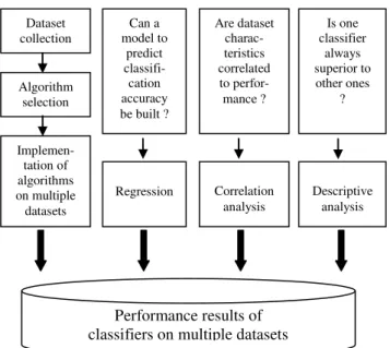
The methodological framework maintained during the research study is shown in Figure 1. Since research study is interested in multiple datasets, in the implementation phase sample datasets have been used. On the experimental datasets, the selected classification algorithms have been implemented. WEKA has been utilised as the tool to run Naïve Bayesian, AIRS, Logistics and MLP algorithms. SPSS has been utilised as the tool to run the Chaid algorithm since it is available in SPSS. The results of the implementations have been tabulated. Afterwards, a descriptive analysis has been conducted to find answers to the first research question. Correlation analysis has been studied to answer the second research question and lastly, a regression model has been built to deal with the third research question.
Figure 1: Methodological Framework
A. Data collection
Sample datasets have been collected from internet repositories, mainly from the UCI Machine Learning Repository. The experimental datasets are Acute, Breast Cancer, Cars, Chess, Credits, Iris, Letters, Red wine, White wine and Wine. Table I summarises the attributes of each dataset.
B. Algorithms
Although many classification models exist, only some have been selected within the scope of this study. The selected algorithms are Naïve Bayesian algorithm, Chaid decision tree algorithm, Multilayer perceptron (MLP), Artificial Immune Recognition Systems (AIRS) and Logistics Regression.
The Naïve Bayesian model defines the classification problem with respect to probabilistic idioms, and supplies statistical methods to classify the instances based on probabilities [8].
In decision tree algorithms, the classification process is summarised by a tree. After the model is built, it is applied to the database [10]. The Chaid algorithm grows the tree by finding the optimal split until the stopping criteria is met with
respect to the chi-squares [1]. It can handle missing values and the target function has discrete outputs [14].
Multilayer perceptron is a type of artificial neural network algorithm which regards the human brain as the modelling tool [8]. It provides a generic model for learning real, discrete and vector target values. The ability to understand the hidden model is hard and training times may be long [14].
As the human natural immune system distinguishes and remembers the intruders, the AIRS algorithm is a cluster-based approach that learns the structure of the data and performs a k-nearest neighbour search [12].
Logistic regression makes use of independent variables to predict the probability of events by fitting the data to a logistic curve [2].
Each algorithm can make use of both numerical and categorical variables as inputs. They can handle target classes with more than two class types. Algorithms can also be referred to as classifiers or models.
Table I: Dataset characteristics
Dataset Name
Number of Variables
Number of Nominal Variables
Number of Numerical Variables
Target Class Types
Number of Instances
acute 7 6 1 2 120
breast
cancer 9 0 9 2 684
cars 6 4 2 4 1727
chess 6 3 3 18 28056
credits 15 9 6 2 653
iris 4 0 4 3 150
letters 16 0 16 26 20000
wineall 11 0 11 7 6497
wine red 11 0 11 6 1599
wine
white 11 0 11 7 4898
C. Implementation
First, data cleaning was applied on the datasets selected. According to the missing data analysis, missing data have been removed from the datasets. Other than missing data analysis, datasets were also cleaned to remove noisy data. Unnecessary space characters or other spelling mistakes were also cleaned in the datasets.
Another usual step in data pre-processing is data discretisation. Although some algorithms are said to perform better when the numerical input variables are discretised [4], in this study numerical variables have not been put into binned intervals in order to maintain the same conditions for all algorithms.
Once the data pre-processing steps have been completed, all 10 datasets (Acute, Breast Cancer, Cars, Chess, Credits, Iris, Letters, Red wine, White wine and Wine) have been used to run the 5 classification algorithms (Naïve Bayesian, Chaid, MLP, AIRS and Logistics algorithms). For all algorithms, splitting the data into train and test splits has been selected as the validation method. 66% of the data has been set as the training part and the rest has been set as the testing part. Then 10-fold cross validation has been implemented on the same Dataset
collection
Can a model to
predict classifi-
cation accuracy be built ?
Are dataset charac- teristics correlated to perfor- mance ?
Is one classifier
always superior to other ones
? Algorithm
selection
Implemen- tation of algorithms on multiple datasets
Regression Correlation analysis
Descriptive analysis
datasets for the selected algorithms. In other words, both splitting and 10-fold cross validation methods have been applied.
IV. EXPERIMENTAL RESULTS AND DISCUSSIONS In this section the performance results of each algorithm on each dataset will be discussed and research questions will be answered accordingly.
When pointing at the performance results of the classifier, its classification accuracy is actually measured. Accuracy is calculated by determining the percentage of instances correctly classified [10]. Costs for wrong assignment can also be applied in classification problems; however, misclassification costs are not within the scope of this study.
The accuracy values of the multiple dataset implementations according to each classifier can be seen in Tables II and III.
Table II: Accuracy results / 10-fold cross validation Airs Chaid Logistics Mlp
Naive Bayes acute 100.0 91.7 100.0 100.0 95.8
breast
cancer 96.2 93.0 96.8 96.0 96.3
cars 94.6 81.9 93.4 99.6 85.2
chess 38.0 39.9 30.8 54.1 34.1
credits 82.5 86.4 86.1 82.7 78.3
iris 95.3 66.7 96.0 97.3 96.0
letters 86.5 53.8 77.4 82.2 64.0
wineall 86.5 53.8 77.4 54.9 64.0
winered 51.3 59.4 59.8 60.7 55.0
winewhite 48.3 54.6 53.7 55.2 44.3
Table III: Accuracy results / 66% train-test split Airs Chaid Logistics Mlp
Naive Bayes acute 100.0 61.9 100.0 100.0 95.1
breast
cancer 96.1 93.2 97.0 96.6 96.1
cars 92.9 81.3 90.5 98.8 87.6
chess 36.6 37.0 32.6 53.8 33.6
credits 78.5 88.1 83.0 79.7 75.3
iris 98.0 23.5 92.2 98.0 94.1
letters 83.6 54.5 77.0 82.8 64.4
wineall 83.6 54.5 77.0 56.3 64.4
winered 51.8 57.7 57.9 62.5 52.0
winewhite 46.0 53.9 52.3 51.2 43.2 A. Research question 1: Does one classifier always outperform the others?
Based on the findings of the empirical study, it can be seen in Tables II and III that the same classifier is not the best one for all datasets and always outperforms the other classifiers. For each dataset the best predictive classifier has been defined. So we can conclude that a classifier cannot be said to outperform the others in every dataset.
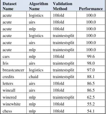
According to Table IV, the overall best accuracy is obtained as 100% in the “acute” dataset. The classifiers producing that rate of accuracy are Logistics, AIRS and MLP.
Table IV: Overall best accuracy results
Dataset Name
Algorithm Name
Validation
Method Performance
acute logistics 10fold 100
acute airs 10fold 100
acute mlp 10fold 100
acute logistics traintestsplit 100
acute airs traintestsplit 100
acute mlp traintestsplit 100
Table V displays the detailed accuracy results for the best result cases of each dataset. Logistics has the best performance for „acute‟ and „breast cancer‟ datasets; AIRS has the best accuracy for „acute‟, „iris‟, „letters‟ and „wine all‟ datasets and lastly, MLP has the best accuracy for „acute‟, „cars‟, „wine red‟, „wine white‟ and „chess‟ datasets. Chaid produces better performance only for the „credits‟ dataset. Interestingly, Naïve Bayesian has never produced the best result for a dataset from those classifiers.
Table V: Best accuracy results for each dataset
Dataset Name
Algorithm Name
Validation
Method Performance
acute logistics 10fold 100.0
acute airs 10fold 100.0
acute mlp 10fold 100.0
acute logistics traintestsplit 100.0
acute airs traintestsplit 100.0
acute mlp traintestsplit 100.0
cars mlp 10fold 99.6
Iris airs traintestsplit 98.0
breastcancer logistics traintestsplit 97.0 credits chaid traintestsplit 88.1
letters airs 10fold 86.5
wineall airs 10fold 86.5
winered mlp traintestsplit 62.5
winewhite mlp 10fold 55.2
chess mlp 10fold 54.1
Table VI: Distribution of classifiers across performance intervals
Performance (Binned)
Total
Low Middle Good Very Good Algorithm
Name
Airs 6 0 8 6 20
Chaid 3 10 7 0 20
Logistics 2 4 9 5 20
Mlp 1 7 4 8 20
Naïve Bayes
4 6 5 5 20
Total 16 27 33 24 100
B. Research question 2: Are dataset characteristics correlated to the performance of classifiers?
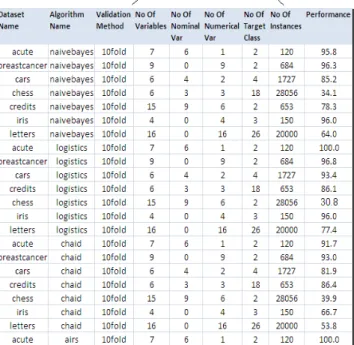
Once all of the iterations have been completed in the implementation step, a dataset of 100 rows including the combinations of the datasets, the algorithms and the validation methods with 9 columns for the variables have been obtained.
The first eight columns in Table VII have been set as input variables, which are dataset name, algorithm name, validation method, number of variables, number of nominal variables, number of numerical variables, number of target class types and number of instances. The last column in Table VII shows the performance variable, which is set as the dependent variable. Since the second research question is interested in dataset characteristics, independent variables have been defined based on dataset attributes such as number of variables, number of nominal variables, number of numerical variables, number of target class types and number of instances.
Table VII: An excerpt from the Results dataset
On the newly created dataset, which is referred to as the Results dataset, some kind of correlation analysis can be
conducted in order to determine if any of the input variables affect the performance results significantly.
Firstly, in order to conduct the correlation analysis, all variables have been coded into numerical variables, and Z-score normalisations have been applied to them. SPSS has been used for implementation.
Table VIII: Correlation between accuracy and number of variables
Performance
Number of Variables Performance Pearson
Correlation
1 -.509** Sig.
(2-tailed)
.000
N 100 100
Number Of Variables
Pearson Correlation
-.509** 1
Sig. (2-tailed)
.000
N 100 100
Table IX: Correlation between accuracy and number of nominal variables
Performance
Number of Nominal Variables Performance Pearson
Correlation
1 -.058
Sig.
(2-tailed)
.566
N 100 100
Number Of Nominal Variables
Pearson Correlation
-.058 1
Sig. (2-tailed)
.566
N 100 100
Table X: Correlation between accuracy and number of numerical variables
Performance
Number of Numerical Variables Performance Pearson
Correlation
1 -.370** Sig.
(2-tailed)
.000
N 100 100
Number of Numerical Variables
Pearson Correlation
-.370** 1
Sig. (2-tailed)
.000
Table XI: Correlation between accuracy and number of target class types
Performance
Number of Target
Class Types Performance Pearson
Correlation
1 -.115
Sig.
(2-tailed)
.255
N 100 100
Number Of Target Class Types
Pearson Correlation
-.115 1
Sig. (2-tailed)
.255
N 100 100
Table XII: Correlation between accuracy and number of instances
Performance
Number of Instances Performance Pearson
Correlation
1 -.564** Sig.
(2-tailed)
.000
N 100 100
Number of Instances
Pearson Correlation
-.564** 1
Sig. (2-tailed)
.000
N 100 100
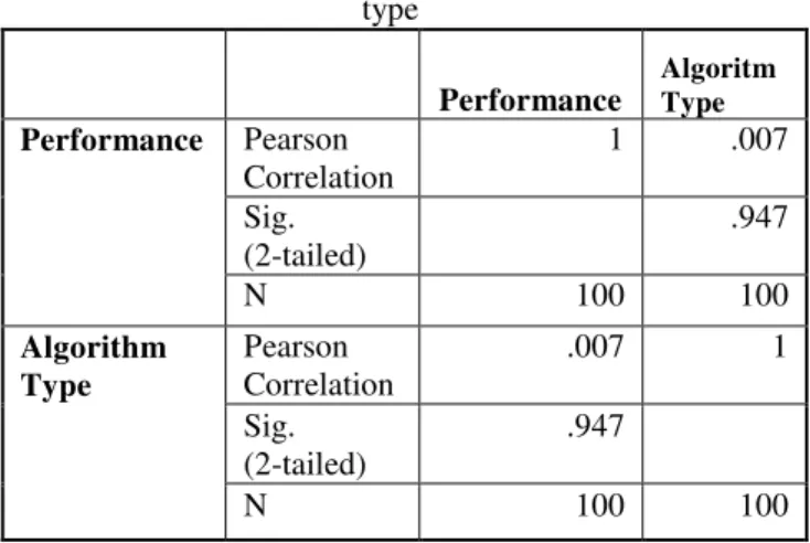
Table XIII: Correlation between accuracy and algorithm type
Performance
Algoritm Type
Performance Pearson Correlation
1 .007
Sig.
(2-tailed)
.947
N 100 100
Algorithm Type
Pearson Correlation
.007 1
Sig. (2-tailed)
.947
N 100 100
Table XIV: Correlation between accuracy and validation methods
Performance
Validation Method Performance Pearson
Correlation
1 -.051
Sig.
(2-tailed)
.611
N 100 100
Validation Method
Pearson Correlation
-.051 1
Sig. (2-tailed)
.611
N 100 100
According to Tables VIII to XIV, some of the input variables have been found to be significantly correlated to the dependent variable, which is the performance of the classifier. Based on these results, the number of variables in the dataset (-0.509 Pearson value), the number of numerical variables in the dataset (-0.370 Pearson value) and the number of instances in the dataset (- 0.564 Pearson value) have been found to go hand in hand with the classifier performance. On the other hand, the number of nominal variables in a dataset, the number of target class types, algorithm name and validation method have been found not to be significantly correlated to classifier accuracy. As a result, the answer to the second question can be concluded in such a way that some of the dataset characteristics can affect the classifier performance.
C. Research question 3: Can a model to predict the classifier performance be built?
A regression model has been developed to answer the last research question. Due to finding the correlations between the selected independent and dependent performance variable in the previous stage, it is important to design a regression model.
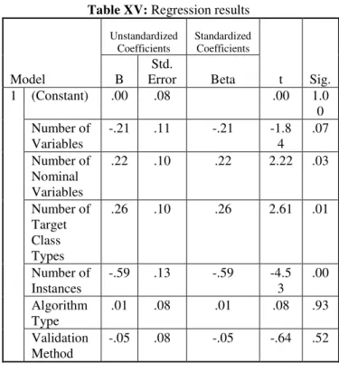
Since there is a Results dataset containing the algorithm and dataset specific attributes in Table XV, it is possible to use these in a regression model and see their causal effects on the dependent performance variable.
According to the regression results, it is possible to build a model to predict the performance result. Figure 2 shows the regression function for predicting the performance.
Figure 2: Regression function
The aim of running a regression is to figure out whether the coefficients on the independent variables are really different from 0; in other words, whether the independent variables are having an observable effect on the dependent variable. If coefficients are different than 0, this means the null hypothesis (the dependent not affected by the
Performance =
-0.210 * Number of Variables
independents) can be rejected. Based on the regression equation in Figure 2, some of the independent variables have been found to affect the dependent variable‟s performance. As a result, the number of variables, number of instances, algorithm type and validation method have a negative effect on performance. On the other hand, the number of nominal variables and number of target classes have a positive effect on the performance.
Within a 95% confidence interval, p values in Table XV should be close to or lower than 0.05 in order to be accepted as significant enough. With respect to p values (sig. column), the effect of the number of nominal variables, number of target class types and number of instances on performance is said to be more certain.
Table XV: Regression results
Model
Unstandardized Coefficients
Standardized Coefficients
t Sig. B
Std.
Error Beta 1 (Constant) .00 .08
.00 1.0
0 Number of
Variables
-.21 .11 -.21 -1.8
4 .07 Number of
Nominal Variables
.22 .10 .22 2.22 .03
Number of Target Class Types
.26 .10 .26 2.61 .01
Number of Instances
-.59 .13 -.59 -4.5
3 .00 Algorithm
Type
.01 .08 .01 .08 .93
Validation Method
-.05 .08 -.05 -.64 .52
V. CONCLUSION
In this study, CHAID, MLP, Logistics, AIRS and Naïve Bayesian classification algorithms have been implemented on 10 datasets.
According to the accuracy results, AIRS, MLP and Logistic Function algorithms proved to have the best performances. However, none of the algorithms can outperform the others in every case.
Another interest has been to find out the correlations between the accuracy results of classifiers and the dataset attributes. Based on the correlation analysis, the number of variables, number of numerical variables and number of instances in the dataset have been found to be significantly correlated with performance.
Based on the findings of this study, it can also be said that a regression model can be built to predict the performance of a classifier on a given dataset.
In this study, the factors affecting the classification algorithm performance have been underlined based on the empirical results of correlation and regression studies. The fact that dataset characteristics influence the accuracy of the algorithm cannot be denied. The deviation of algorithm accuracies across different datasets is observable. The
business and academic community should take these results into consideration, since establishing a knowledge discovery process on the same algorithm may not always be certain. The model assessment and selection phase should be paid the utmost attention in an iterative manner, because any difference in dataset characteristics can change the model‟s accuracy, and switching to another classifier may be a better decision. The regression model also gives some hints about the importance of a dataset, and that the accuracy can be predicted based on the instances or the field attributes of the dataset.
It is not an easy task to decide which classifier to use in a data mining problem; thus this study shows the importance of model selection and explains that an algorithm is not the best choice for all datasets.
Certainly, conclusions are based on the scope of this study; therefore, increasing the scope may help to develop an extended framework for predicting the accuracy of classifiers. Obviously, there may be other factors influencing the accuracy of a model, thus input variables of the regression function should be increased in the future.
REFERENCES
[1] A. Berson, S. Smith, K. Thearling, Building Data Mining Applications for CRM. McGraw Hill, 1999, pp.166.
[2] D.Hand, H.Mannila, P.Smyth, Principles of Data Mining. Cambridge: The MIT Press, 2001, pp.140-352.
[3] E. Keogh, S. Kasetty, “On the Need for Time Series Data mining benchmarks: a survey and empirical demonstration”, Data Mining and Knowledge Discovery, Vol. 7, pp. 349-371.
[4] Ge, E., Nayak, R., Xu, Y. and Li, Y., “Data mining for lifetime prediction of metallic components”, In Proc. Fifth Australasian Data Mining Conference (AusDM2006), Sydney, Australia, 2006. [5] He, H., Jin, H., Chen, J., McAullay, D., Li, J. and Fallon, T., “Analysis
of breast feeding data using data mining methods”, In Proc. Fifth Australasian Data Mining Conference (AusDM2006), Sydney, Australia, 2006.
[6] J. Han, M. Kamber, Data Mining Concepts and Techniques. 2nd ed., Academic Press, Morgan Kaufmarm Publishers, 2005, pp.5-360. [7] J. R. Quinlan, "Comparing connectionist and symbolic learning
methods," in Computational Learning Theory and Natural Learning Systems: Constraints and Prospect, vol. 1, S. J. Hanson, G. A. Drastal, and R. L. Rivest, Ed. Cambridge: MIT Press, 1994, pp. 445–446. [8] K. J. Cios, W. Pedrycz, R. W. Swiniarski, L. A. Kurgan, Data Mining A
Knowledge Discovery Approach. USA: Springer, 2007, pp.52-440. [9] L. P. Kaelbling, "Associative methods in reinforcement learning: an
emprical study," in Computational Learning Theory and Natural Learning Systems: Intersection Between Theory and Experiment, vol. 2, S. J. Hanson, T. Petsche, M. Kearns and R. L. Rivest, Ed. Cambridge: MIT Press, 1994, pp. 145–153.
[10] M. H. Dunham, Data Mining Introductory and Advanced Topics. New Jersey: Prentice Hall, 2002, pp.75-92.
[11] O. Maimon, L.Rokach, The Data Mining and Knowledge Discovery Handbook. USA: Springer, 2005, pp.150.
[12] P. v.d. Putten, L. Meng, J. N. Kok, “Profiling novel classification algorithms: Artificial Immune System”, Available: http://www.liacs.nl/~putten/library/200809vdPuttenKokMengCIS.pdf, Retrieved 2009-12-01.
[13] S. Hacker, L.v. Ahn, “Matchin: eliciting user preferences with an online game”, In CHI '09: Proceedings of the 27th international conference on Human factors in computing systems, New York, USA, ACM, 2009.
[14] T. M. Mitchell, Machine Learning. McGraw Hill, 1997, pp.54-85. [15] W. Finnoff, F. Hergert, H. G. Zimmermann, "Improving model