Enrique Martínez-Galán*; Isabel Proença*; Maria Paula Fontoura* TRADE POTENTIAL REVISITED: A PANEL DATA
ANALYSIS FOR ZIMBABWE
WP14/2015/DE/UECE/CEMAPRE
_________________________________________________________ De pa rtme nt o f Ec o no mic s
W
ORKINGP
APERS1
TRADE POTENTIAL REVISITED: A PANEL DATA ANALYSIS FOR ZIMBABWE
Enrique Martínez-Galán*
School of Economics and Management and Portuguese (ISEG), Universidade de Lisboa, and Portuguese Finance Ministry.
Isabel Proença*
School of Economics and Management and Portuguese (ISEG) and CEMAPRE, Universidade de Lisboa
Maria Paula Fontoura*
School of Economics and Management and Portuguese (ISEG) and UECE, Universidade de Lisboa
ABSTRACT
This paper notes that previous results on trade potential based on a panel data set may be biased and proposes the adequate Poisson Pseudo Maximum Likelihood method to estimate trade potential based on the elasticity estimates generated by a gravity model, with conclusions on trade potential based on confidence intervals estimated with the Delta method. This approach had not been yet considered in the literature for panel data. This methodology is used to evaluate Zimbabwe export potential in a period characterized by strong restrictions on trade, based on the elasticity estimates generated by an augmented gravity model for six Southern African Development Community member countries and their exports to the rest of the world. Results show that Zimbabwe has a large unexploited trade potential which will not be realized without political stability and structural reforms. For comparison purposes, we also present the gravity coefficients calculated with other estimation methods.
JEL Classifications: F14, F15, F16
Keywords: gravity model, export potential, Poisson Pseudo-Maximum Likelihood estimator, panel data, confidence intervals, Delta method, Zimbabwe, Southern Africa Development Community.
2 INTRODUCTION
Evaluation of the trade potential between countries or groups of countries is usually based on the well-diffused method of estimating a log-linearised version of a gravity model and using the parameters to project expected trade, which is compared with observed trade1 The assumption is that potential trade is equal to fitted trade (“expected” trade), i.e. trade projected by using the coefficients of the estimated gravity model. If the ratio between fitted trade and observed trade is higher than one, the conclusion is that the country may expand trade in the future; if instead it is lower than one, the increase in trade flows is only possible if the country improves some of its characteristics.
Three shortcomings to this traditional procedure on predicting trade need, however, to be highlighted.
First, Santos Silva and Tenreyro (2006) argue that estimation of the gravity model using Ordinary Least Squares (OLS) and the log transformation may be inconsistent in the presence of heteroscedasticity. They instead recommend the estimation of the gravity equation by Poisson Pseudo Maximum Likelihood (PPML), a method scarcely used in previous papers. Their conclusion is drawn for cross-section data but it can be easily extended to panel data, where the same units are observed for several periods of time.
Second, even if the log-linear equation is consistently estimated, it leads to the consistent estimation of the expected log of trade. However, trade potential is based on the estimated expected trade. Because of Jensen inequality, expected trade is not just the exponential of the expected log of trade and it in fact tends to be higher than the latter. Therefore, the usual procedure consisting on estimating trade potential based on exponentiation of the projections given by the log linear model displays, in general, a negative bias.
Third, accuracy of predictions depends on sampling variation of the ratio between projected and observed trade, which can be accounted for by means of confidence intervals. Breuss and Egger (1999) are the first, and the few, to do so. However, they use the OLS estimator with cross-section data and they obtain huge interval spreads that unable to draw unequivocal conclusions on the potential of trade of a country. The problem with their result is not only that they make use of an estimation method that may be inadequate, but also that they are considering ill-suited prediction intervals. Indeed, the large confidence intervals obtained by those authors are a typical result of predicting the individual behavior of the country pair trade without taking into account that prediction intervals for an individual country are commonly large when data is quite heterogeneous (which is the case of most trade data).This happens due to the large uncertainty arising from the individual idiosyncratic unobserved error term.
3
confidence intervals for that mean trade as the base of inference for trade potential. The reasoning is that prediction intervals for the mean are more reliable and precise since they overcome that sort of uncertainty detected in Breuss and Egger (1999) approach. Because aggregate flows are a sum of non-linear functions of the parameters, Proença et al (2008) adopted the Delta method to calculate the variance of the preditictions2.
Proença et al (2008) approach not only leads to confidence intervals with reasonable lengths but it also allows a clearer interpretation of the trade potential results: if a ratio higher than one is not rejected, one can conclude that observed trade is below the average and therefore, the country may expand future trade by employing more efficiently its trade determinants; if a ratio lower than one is not rejected, the country has only scant possibilities of improving its trade as it is already operating above the average (op. cit, pp. 207-8).
This paper estimates a gravity model to determine trade potential with the adequate PPML method and, additionally, conclusions on trade potential are based on prediction intervals built according to Proença et al (2008) approach, i.e. we use the mean trade flow and the Delta method to estimate the variance of the predictions. However, unlike these authors, who have built a cross section model, in this paper we opt for a panel data set; such an approach had not been yet considered in the literature for panel data, to the best of our knowledge.
To control for country-pair unobserved heterogeneity we opt for the PPML with random effects and Mundlak device. The latter intends to correct for an eventual dependency between the unobserved heterogeneity term and the explanatory variables. This approach was used in Proença et al (2015) to explain trade flows within the European Union together with a semiparametric extension, and also had never been adopted to calculate trade potential.
To exemplify the approach that we propose, we estimate Zimbabwe´s export potential with a panel data set including nine Southern Africa Development Community (SADC) member countries and their exports to their 50 major world trading partners between 2007 and 2011. The estimates are then used to predict, out of sample, Zimbabwe’s exports to those destinations, as explained by the force its economy exerts within world trade on grounds of the market size (economic mass) and the “distance” from other markets, measured by factors such as geographical distance and the existence of cultural, language and other specific ties with trading partners.
4
2. MODEL SPECIFICATION OF THE GRAVITY MODEL
The gravity model for panel data to be used in the empirical study is based on the following equation:
0
| , , , exp log( ) log( )
ijt ijt ij ij ij ijt ij ij ij t ijt
E T x Dist D x β Dist D γ u
where Tijtis trade from country ito country jat timet, xijtis a vector of time-varying explanatory variables, Distijis the distance between countries iand j, Dijis a vector of (time-invariant) Dummy variables, ijis a random effect rendering the unobserved
heterogeneity in trade specific to each bilateral partner,
t is the fixed time effect,ijt
u is the idiosyncratic error term, while
0, β,
andγare unknown parameters to be estimated. To prevent from inconsistency in estimation due to an eventual correlation between the unobserved heterogeneity term and the explanatory variables the approach of Mundlak(1978) is used which amounts to assume that the means of the explanatory variables that vary in time capture all the dependency between the unobserved heterogeneity term,ij, and the regressors according to the following specificationij log(xijt)' aij
with log( ijt) 1 / T1log( ijt) t
T x
x and aij a pure unobserved random effect with a
known distribution form verifyingE a ij |xij1,...,xijT,Distij,Dij 0 and a vector of parameters to be estimated. Therefore, the panel data gravity equation becomes
' 0
| , , , exp log( ) log( ) log( )
ijt ijt ij ij ij ijt ij ij ijt t ij ijt
E T x Dist D a x β Dist D γ x a u
(1)
Assuming that the conditional expectation in (1) is well specified and that exp(aij)is distributed as Gamma( , ) and independent of the other explanatory variables, the unknown parameters in (1) can be estimated by Poisson Pseudo Maximum Likelihood known as Poisson panel regression (panel PPML) with random effects. Given that trade data is not truly Poisson distributed and, therefore, only the mean is correctly specified, variances have to be estimated robustly to misspecification in order to make inference valid.
3. AN EMPIRICAL EXAMPLE: ZIMBABWE’S TRADE POTENTIAL
5
explain the expectation of a large unexploited trade potential of the country in the period analyzed. Next we show data on Zimbabwe´s external trade, with a special emphasis on exports. Finally, section 3.2 presents the estimates for Zimbabwe´s export potential to fifty destination countries.
3.1. An overview of Zimbabwe´s history and external trade
Zimbabwe achieved de jure sovereignty from the United Kingdom in April 1980, after more than a decade of soft guerrilla that followed the unilateral declaration of independence in 1965. By that time, in 1966, the former Rhodesia was the first autonomous state where the United Nations imposed a mandatory trade embargo to, which was extended two years later in 1968. After a difficult post-independence two decades, with coexisting of an authoritarian regime and civil unrests, the mandatory confiscation and land redistribution of farmland initiated in 2000, which evicted more than 4,000 white farmers, led to a sharp decline in agricultural exports of a country once considered as the farmland of Africa. As a result, Zimbabwe experienced a severe currency shortage that led to hyperinflation and chronic critical deficiency in imported fuel and consumer goods. Inflation rose from an annual rate of 16 per cent in 1996 to an official estimate of 231,150,889 per cent in July 2008 3, after which conventional inflation measures stopped being published.
Moreover, a wide range of sanctions were imposed by the United States government and the European Union (EU) in 2001 and 2002 against President Mugabe and his regime, charged with committing numerous human rights abuses,
electoral irregularities and pre-election violence. These sanctions meant de facto a
trade embargo, in particular regarding business owned or controlled by government officials, with huge consequences for the economy. In 2002 Zimbabwe was suspended from the Commonwealth of Nations and the government had its lines of credit at international financial institutions frozen.
The food and economic crisis, together with an HIV/AIDS epidemic, a drought that affected the entire country and the Zimbabwe’s involvement in the war in the Democratic Republic of Congo from 1998-2002, led to economic collapse, a formal 80 per cent unemployment rate and a dramatic humanitarian crisis (life expectancy at birth for males dramatically declined from 60 years in 1990 to 42 years in 2010). Real gross domestic product (GDP), which had already decreased by five percent in 2000, recorded a cumulated fall of 43.5 per cent in the next eight years, with two peaks of negative growth higher than 17 per cent in 2002 and 2008 (OECD, 2004 and AfDB, 2012). In 2008, the country’s economy had lost nearly 56 per cent of its annual production when compared to 2000 and industries were operating at only 20 to 30 per cent of their capacity.
6
including the euro, the sterling Pound, the South African rand and the Botswana’s pula. Real GDP inverted the previous negative tendency and grew by about 6 per cent in 2009 and 9 per cent in 2010 (AfDB, 2012) buoyed by high mineral prices and the improving agricultural sector. In November 2010, the IMF described the Zimbabwean economy as "completing its second year of buoyant economic growth after a decade of economic decline", briefly citing "strengthening policies" and "favorable shocks" as main reasons for the economic growth (IMF, 2010). By the end of October 2012, the IMFannounced the relaxation of restrictions on technical assistance opening way for future staff-monitored reform programs (IMF, 2012).
The turn of the decade brought in addition some important signs of openness in the external front. The EU provisionally started implementing a new commercial partnership agreement with Zimbabwe in May 2012, together with Madagascar, Mauritius and Seychelles (EU, 2009). These countries will gradually open their markets to European exports over the course of 15 years. The deal implies that the EU will allow products imported from its partners on its markets without applying any special taxes or quotas (no tax, no quota). Furthermore, the EU foreign minister stated in 2012 that the Union was available to suspend most sanctions against Zimbabwe once it has held a credible referendum on a new constitution (EU, 2012). As a new constitution was approved by an overwhelming majority in an incident-free referendum in 16 March 2013, the EU officially suspended sanctions with Zimbabwe on 25 March 20134, while the World Bank and the African Development Bank Groups initiated re-engagement processes with Zimbabwe by providing technical assistance and institutional capacity building..In addition, in 2010 was created the Zimbabwe Multi-Donor Trust Fund, managed by the African Development Bank, with approximately USD 9 million to invest, at least initially, in water supply and sanitation rehabilitation and energy infrastructures.
There is hope in the international community that the Zimbabwe has started a period of national reconciliation and peaceful activity that can lead the country to implement the needed reforms. According to World Bank 5, agriculture, mining and banking are key sectors where reforms are necessary. In agriculture, a transparent framework for the adjudication of land rights will be important to making Zimbabwe’s farms more productive. Landholders need to obtain title to their property in order to build a private property market in Zimbabwe and unlock access to credit for farmers. In mining, the poor transparency in the mineral sectors deprives the government of revenue that it could invest in people and infrastructure, and the authorities are urged to move forward on efforts to update the legislative and regulatory framework for mining. With regard to banking, the recent authorities’ decision to strengthen capital requirements must be welcomed and banking supervision must also be strengthened to address signs of deteriorating portfolio performance in certain banks
7
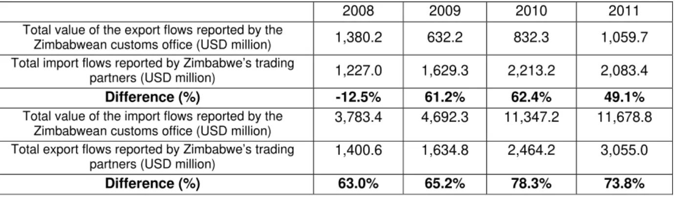
Data on Zimbabwe as reported by its trading partners to the United Nations Statistical Department are derived from a world trade matrix compiled from COMTRADE at five digits of the Standard Industry Trade Category (SITC) classification, rev. 4. We believe that this is the proper way to assess Zimbabwe’s trade, due to the fact that Zimbabwe consistently ranks in the lowest positions in country classifications in quality of public institutions, governance and political stability. The difference between the total value of the trade flows reported to the United Nations Statistical Department by the Zimbabwean customs office and the mirrored flows reported by its trading partners is in fact relatively high (see table 1 below).
Table 1 – Comparison between the total value of the trade flows reported by the Zimbabwean customs office and the total value of those same flows when reported by Zimbabwe’s trading partners
2008 2009 2010 2011
Total value of the export flows reported by the
Zimbabwean customs office (USD million) 1,380.2 632.2 832.3 1,059.7
Total import flows reported by Zimbabwe’s trading
partners (USD million) 1,227.0 1,629.3 2,213.2 2,083.4
Difference (%) -12.5% 61.2% 62.4% 49.1%
Total value of the import flows reported by the Zimbabwean customs office (USD million)
3,783.4 4,692.3 11,347.2 11,678.8
Total export flows reported by Zimbabwe’s trading partners (USD million)
1,400.6 1,634.8 2,464.2 3,055.0
Difference (%) 63.0% 65.2% 78.3% 73.8%
Source: Authors’ estimation based on UNCOMTRADE, accessed on 6 February 2013.
The table above also shows that exports inverted their decreasing trend in 2009, rising from USD 1.6 billion in 2009 to USD 2.1 billion in 2011. Imports also increased in terms of their growth rate in the same period from USD 1.6 billion to USD 3.1 billion, respectively. These increases, of 31 per cent and 94 per cent, respectively for exports and imports, can be interpreted as being a result of the improvement in Zimbabwe’s political situation and the start of the uplifting of at least some of the abnormal hurdles that were constraining both the country’s economy and its trade flows. As it would have been expected, the demand for foreign goods increased much more quickly than the capability to export, as the latter depends for critically in the country’s infrastructures and productive capacity.
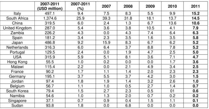
8
Table 2 – Zimbabwe’s twenty largest importing countries (2007-2011, cumulated)
2007-2011 (USD million)
2007-2011
(%) 2007 2008 2009 2010 2011
Italy 497.1 9.4 7.5 8.3 5.5 9.9 15.2
South Africa 1,374.6 25.9 39.3 31.8 18.1 13.7 14.5
China 319.5 6.0 2.4 1.3 6.7 13.6 10.6
United Kingdom 287.0 5.4 3.6 3.8 10.5 4.1 7.9
Zambia 226.2 4.3 0.0 4.3 7.4 6.4 6.3
Spain 181.2 3.4 2.3 3.5 1.6 3.5 5.8
Japan 486.8 9.2 15.9 8.3 6.7 6.2 5.2
Netherlands 316.3 6.0 6.4 3.7 8.8 7.8 5.2
Portugal 129.5 2.4 0.0 1.9 4.7 2.5 5.0
USA 315.9 5.9 5.1 8.1 3.6 7.1 4.7
Hong Kong 55.5 1.0 0.2 0.0 0.0 1.7 3.6
Malawi 115.4 2.2 0.0 2.1 4.9 3.4 2.5
France 90.2 1.7 1.1 1.4 2.0 2.3 2.3
Germany 195.1 3.7 5.5 3.7 4.2 3.0 1.5
Jordan 97.4 1.8 1.9 1.4 3.2 2.6 1.0
Belgium 56.7 1.1 1.0 0.5 2.7 1.4 0.7
South Korea 79.4 1.5 2.7 2.3 0.5 01 0.6
Namibia 54.6 1.0 1.3 2.0 0.7 0.2 0.2
Singapore 37.1 0.7 0.9 0.4 1.5 1.1 0.1
Sudan 93.8 1.8 0.0 6.8 0.0 0.0 0.0
Source: Authors’ estimation based on UNCOMTRADE, accessed on 6 February 2013.
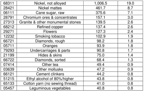
Zimbabwe’s export basket can be described as basically consisting of natural resources. Mining represented more than 55 per cent of the country’s exports between 2007 and 2011. Together with food, livestock, beverages, tobacco and crude materials, they represented 82 per cent. Ferrochromium and nickel only represented almost half of total Zimbabwean exports in that same period (see table 3 for a brief view of Zimbabwe’s export structure, and also table 4 for a more disaggregated presentation).
Table 3 – Zimbabwe’s exported goods (2007-2011, total, cumulated)
Sector 2007-2011
(USD million)
2007-2011 (%)
Mining 2,946.2 55.5
Food, livestock, beverages and tobacco 953.9 18.0
Manufactured goods 614.6 11.6
Crude materials (wood, seeds, pulp, crude fertilizers) 454.9 8.6
Machinery and transport equipment 225.0 4.2
Chemicals 94.3 1.8
Mineral fuels 21.9 0.4
Source: Authors’ estimation based on UNCOMTRADE, accessed on 6 February 2013.
Table 4 – Zimbabwe’s twenty largest exported goods (5-digit SITC rev. 4) (2007-2011, cumulated)
Code Good 2007-2011
(USD million)
2007-2011 (%)
9
68311 Nickel, not alloyed 1,006.5 19.0
28421 Nickel mattes 461.7 8.7
06111 Cane sugar, raw 375.6 7.1
28791 Chromium ores & concentrates 157.1 3.0
27313 Granite & other monumental stones 139.5 2.6
68212 Refined copper 137.4 2.6
29271 Flowers 127.3 2.4
12232 Smoking tobacco 102.9 1.9
66721 Diamonds, rough 98.2 1.8
05711 Oranges 93.9 1.8
79293 Undercarriages & parts 90.8 1.7
21199 Hides & skins 75.0 1.4
66722 Diamonds, sorted 68.4 1.3
07414 Other tea 49.4 0.9
03639 Other mollusks 47.2 0.9
66121 Cement clinkers 44.2 0.8
51215 Ethyl alcohol of 80%/higher 43.8 0.8
65133 Cotton yarn (no sewing thread) 41.0 0.8
05457 Leguminous vegetables 40.8 0.8
Source: Authors’ estimation based on UNCOMTRADE, accessed on 6 February 2013.
The composition of exports does not vary much by trading partner, with only a few exceptions presenting a more diversified demand, such as Zambia (see table 5 below).
Table 5 – Main imports by Zimbabwe’s eleven largest importing countries (2007-2011, cumulated)
2007-2011 (USD million)
2007-2011
(%) Main imports
South Africa 1,374.6 25.9 Nickel (63.8%)
Italy 497.1 9.4 Ferrochromium (71.5%), Granite & other monumental stones (19.1%)
Japan 486.8 9.2 Nickel (75.4%), Ferrochromium (21.0%)
China 319.5 6.0 Chromium ores (45.0%), Ferrochromium (41.6%)
Netherlands 316.3 6.0 Flowers (32.0%), Ferrochromium (28.6%), Oranges (16.3%)
USA 315.9 5.9 Ferrochromium (55.1%), Nickel (25.3%)
United Kingdom 287.0 5.4 Cane sugar (52.2%), Diamonds (31.3%)
Zambia 226.2 4.3 Cement (15.0%), Coal (6.9%), Fish (6.0%)
Germany 195.1 3.7 Copper (50.7%)
Spain 181.2 3.4 Ferrochromium (60.6%), Cane sugar (19.9%)
Portugal 129.5 2.4 Cane sugar (96.7%)
Source: Authors’ estimation based on UNCOMTRADE, accessed on 6 February 2013.
10 3.2. Estimating trade potential
The counterfactual sample
The basis for predicting Zimbabwean export volumes are the elasticity estimates generated by the gravity model fitted to the observed exports of nine SADC countries to fifty destination countries. The fifty target markets represent 87.7 per cent of the sample country exports and 94.1 per cent of world exports. The predictions are out-of-sample as observations for Zimbabwe are excluded from the benchmark regressions.
The reference countries selected as counterfactual were Angola, Botswana, Democratic Republic of Congo, Malawi, Mozambique, Namibia, South Africa, United Republic of Tanzania and Zambia. Other SADC member countries were excluded from the sample due to their small size (Lesotho and Swaziland) or for being islands (Madagascar, Mauritius and Seychelles).
Trade data for these nine countries is not always complete. As in the case of Zimbabwe, they can, at the very least, be described as patchy. Fortunately, trade transactions are typically recorded twice: once by the exporting country when the merchandise is leaving its territory and a second time by the importing country when it enters through customs. Following on this rationale, very detailed merchandise trade statistics can be compiled to the extent that trading partners have been reporting these transactions. This is typically the case for these nine countries. The compilation of relevant data from the point of view of the trading partners instead of following the reporting made by the SADC country allows us to increase the total number of observations for the five years in study from 1,117 to 1,854.
Within the relative homogeneity provided by the SADC framework, these nine countries are similar enough in terms of socio-economic framework and export structure to provide a reasonable benchmark for the trade determinants of Zimbabwean exports, had there been no sanctions and less political instability.
Table 6 below records the main exports of the sample countries in 2010, showing they are basically based on mining and other natural resources, even in the case of South Africa, despite the latter displaying a more diversified industrial base. Note that, by considering the 4-digit level of disaggregation, we conclude that the item "non-metallic mineral manufactures" consists almost entirely of diamonds (88 per cent in the case of Botswana, 99 per cent in the case of Namibia, and even 92 per cent in the case of South Africa), so it’s fair to state that the main exports from all the countries in the sample are specialized in natural resources (with the only exception being the "road vehicles" produced by South Africa, with 7.3 per cent of the total).
Table 6: Main exports by sample countries (2-digit SITC rev. 4) (2010)
Main exports
11
South Africa Non-ferrous metals (15.1%), Metalliferous ores (13.3%), Iron and steel (8.1%), Road vehicles (7.3%), Gold (6.8%), Non-metallic mineral manufactures (6.7%)
Democratic
Republic of Congo Non-ferrous metals (44%), Metalliferous ores (30.3%), Inorganic chemicals (3.4%)
Mozambique Non-ferrous metals (51.3%), Electric current (7.5%), Metalliferous ores (6.3%), Gas (5.1%), Tobacco and tobacco manufactures (4.8%)
Malawi
Tobacco and tobacco manufactures (56.1%), Coffee, tea, cocoa, spices, and manufactures thereof (7.7%), Inorganic chemicals (6.8%), Sugars, sugar preparations and honey (6.2%), Vegetables and fruit (5.7%),
Metalliferous ores (4.6%)
Tanzania Metalliferous ores (16.9%), Vegetables and fruit (12.5%), Coffee, tea, cocoa, spices, and manufactures thereof (9.9%), Tobacco and tobacco manufactures (9.3%), Non-ferrous metals (7.9%), Fish (7.4%)
Zambia Non-ferrous metals (80.5%), Tobacco and tobacco manufactures (4.4%)
Namibia Inorganic chemicals (27.4%), Non-ferrous metals (21.9%), Non-metallic mineral manufactures (19.2%), Fish (12.2%), Metalliferous ores (6.8%)
Botswana Non-metallic mineral manufactures (60%), Metalliferous ores (23.1%), Meat and meat preparations (2.6%) Source: Authors’ estimation based on UNCOMTRADE, accessed on 7 March 2013.
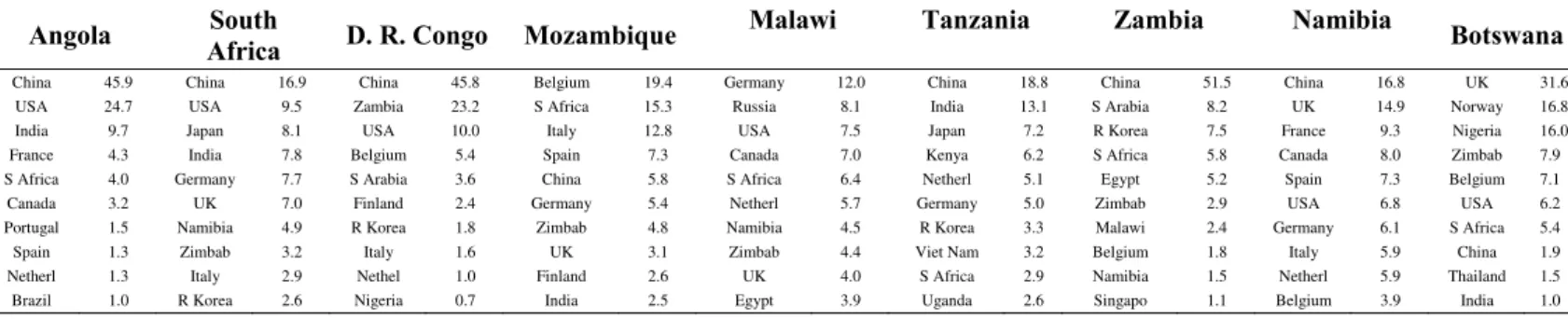
Table 7 presents the largest target markets of the countries in the sample in 2010. As expected, there are differences among them. Nonetheless, the similarities prevail once more. The destination markets consist primarily of industrialized and emerging countries, which is characteristic of countries with the above presented export structure. Noteworthy is the general importance of the People’s Republic of China as a destination market, which in the case of Zimbabwe already ranked first in 2010, together with South Africa (see table 2 above). A less prominent presence of the People’s Republic of China is only observed in Mozambique, Malawi and Botswana.
Table 7: Largest destination markets of the sample countries by decreasing order
(% of country total, 2010)
Angola South
Africa D. R. Congo Mozambique
Malawi Tanzania Zambia Namibia Botswana
China 45.9 China 16.9 China 45.8 Belgium 19.4 Germany 12.0 China 18.8 China 51.5 China 16.8 UK 31.6 USA 24.7 USA 9.5 Zambia 23.2 S Africa 15.3 Russia 8.1 India 13.1 S Arabia 8.2 UK 14.9 Norway 16.8 India 9.7 Japan 8.1 USA 10.0 Italy 12.8 USA 7.5 Japan 7.2 R Korea 7.5 France 9.3 Nigeria 16.0 France 4.3 India 7.8 Belgium 5.4 Spain 7.3 Canada 7.0 Kenya 6.2 S Africa 5.8 Canada 8.0 Zimbab 7.9 S Africa 4.0 Germany 7.7 S Arabia 3.6 China 5.8 S Africa 6.4 Netherl 5.1 Egypt 5.2 Spain 7.3 Belgium 7.1
Canada 3.2 UK 7.0 Finland 2.4 Germany 5.4 Netherl 5.7 Germany 5.0 Zimbab 2.9 USA 6.8 USA 6.2 Portugal 1.5 Namibia 4.9 R Korea 1.8 Zimbab 4.8 Namibia 4.5 R Korea 3.3 Malawi 2.4 Germany 6.1 S Africa 5.4
Spain 1.3 Zimbab 3.2 Italy 1.6 UK 3.1 Zimbab 4.4 Viet Nam 3.2 Belgium 1.8 Italy 5.9 China 1.9 Netherl 1.3 Italy 2.9 Nethel 1.0 Finland 2.6 UK 4.0 S Africa 2.9 Namibia 1.5 Netherl 5.9 Thailand 1.5
Brazil 1.0 R Korea 2.6 Nigeria 0.7 India 2.5 Egypt 3.9 Uganda 2.6 Singapo 1.1 Belgium 3.9 India 1.0 Source: Authors’ estimation based on UNCOMTRADE, retrieved on 7 March 2013.
Explanatory Variables
12
recorded by the fifty trading partners of the selected SADC members in 2001 according to UN COMTRADE database. The dependent variable Xij will be therefore
the nominal import (cif) flows of country j from country i of manufactured products,
measured in millions of US dollar, current prices, accessed from UN COMTRADE.
With regards to the independent variables, the GDP and GDP per capita (GDPpc) of countries involved in the bilateral trade flows are used as proxies for the “economic mass” variables. The intensity of bilateral trade variables is also captured by an absolute distance variable between both countries (DIST), namely the distance between capitals, which is assumed to be a proxy for the “economic centre” of a country. We added dummy variables to capture both countries sharing a common border (CONTIG), the same official language (COMLANG_OFF), a language spoken at least by 20 % of the population (COMLANG_ETHN), the same colonizer (COLONY), and if they belong to the same free trade area (FTA).
The GDP variables are calculated at market exchange prices (MES), following the argument of authors such as Gros and Gonciarz (1996) or Frankel (1997), according to which the proper measure of a country’s trade potential should be based on the international value of goods and services and not on how affluent its inhabitants are, as would be the case if GDP were calculated in terms of purchasing power parity (PPP).
Another question that has arisen in the literature is whether trade values and GDP data should be expressed in nominal or real terms. However, as summarized
by Shepherd (2012), trade flows should be in nominal, not real, terms. The reason
is that these variables are already deflated by the multilateral resistance terms, which are unobserved price indices.
All the above variables are expected to promote bilateral trade flows with the exception of CONTIG, which is expected to be negatively correlated with trade.
The Appendix presents the list of countries included in the data set (A.1) the variables introduced in the gravity model including their statistical sources (A.2) and
table 8 shows the descriptive statistics of the variables.
Table 8 – Descriptive statistics
Variable Mean Std. Dev. Min Max N
Xij 288506.8 1399665.00 0.00 2.49E+07 2077
GDPi 5.67E+10 1.04E+11 4.28E+09 4.09E+11 2077 GDPj 1.10E+12 2.05E+12 3.65E+09 1.51E+13 2077
POPi 2.42E+07 2.03E+07 1767758.00 7.26E+07 2077 POPj 9.85E+07 2.48E+08 764049.80 1.35E+09 2077
DISTW 7466.44 3240.29 0 15491.10 2077
CONTIG 0.04 0.19 0 1 2077
COMLANG_ETHN 0.25 0.43 0 1 2077
COMLANG_OFF 0.24 0.43 0 1 2077
COLONY 0.02 0.15 0 1 2077
COMCOL 0.12 0.33 0 1 2077
13 Econometric results
Estimations were performed with STATA. Results are included in table 9. The simple pooled PPML regression, that ignores the existence of country unobserved heterogeneity, was included for comparison. For the panel PPML with random effects, variances were corrected by panel bootstrap using 10000 replicas. Both regressions control the effect of time by including time dummies.
Table 9 – Estimates of the gravity equation
PPML with random effects and Mundlak device
(1)
Pooled PPML (2)
Bootstrap Robust
Coef.
Std.
Err. z P>z Coef. Std.
Err. z P>z
constant -27.164 3.254 -8.35 0.000 -30.198 4.683 -6.45 0.000
lGDPi 0.838 0.229 3.67 0.000 0.989 0.100 9.85 0.000
lGDPj 0.871 0.330 2.64 0.008 0.766 0.207 3.71 0.000
lpopi -1.935 2.879 -0.67 0.501 -0.211 0.122 -1.72 0.085
lpopj -1.365 1.800 -0.76 0.448 0.413 0.199 2.08 0.037
lDistW -1.198 0.285 -4.20 0.000 -0.730 0.475 -1.54 0.124
contig 1.069 0.421 2.54 0.011 2.101 0.829 2.53 0.011
comlang_ethn. -0.076 0.296 -0.26 0.798 -0.480 0.366 -1.31 0.190
comlang_off 0.466 0.291 1.60 0.110 0.200 0.307 0.65 0.515
colony 0.987 0.483 2.04 0.041 1.032 0.339 3.04 0.002
comcol -0.499 0.370 -1.35 0.178 -0.502 0.477 -1.05 0.292
FTA 1.041 0.380 2.74 0.006 0.176 0.342 0.51 0.608
y2008 0.132 0.065 2.03 0.042 0.083 0.047 1.78 0.075
y2009 -0.165 0.122 -1.36 0.174 -0.244 0.071 -3.45 0.001
y2010 -0.063 0.188 -0.33 0.739 -0.255 0.092 -2.77 0.006
y2011 -0.060 0.252 -0.24 0.812 -0.329 0.149 -2.20 0.028
lGDPibar 0.183 0.247 0.74 0.458
lGDPjbar 0.054 0.335 0.16 0.872
lpopibar 1.773 2.876 0.62 0.537
lpopjbar 1.486 1.802 0.82 0.410
Number of obs. 1812 1812
Log pseudo-lik. -21752080 -368185456
R-squared 0.171 0.433
Notes: Bootstrap standard errors were obtained with 10000 Bootstrap replications based on 456 clusters. Robust standard errors are robust by 456 clusters. Variables lGDPibar, lGDPjbar, lpopibar, lpopjbar are equal to the average of lGDPi, lGDPj, lpopi, lpopj respectively for each country i and j in the observed period and result from the Mundlak device to control from an eventual endogeneity in the random effect. R-squared was calculated as the square of the empirical correlation coefficient between the observed and the fitted exports.
14
within the same free trade area. These effects are statistically significant at 5%. On the other hand, variables like population, the existence of an official common language or a common language spoken by a minority in the other country and the existence of a common colonizer have no statistically significant effect in exports.
Comparing to the pooled PPML there are some differences that deserve to be mentioned indicating that to control for unobserved heterogeneity with and eventual dependency of explanatories may be an important issue in the gravity equation estimation for panel data to prevent from inconsistency in estimation. These differences concern the effect of population of exporter and importer countries, which are statistically significant (the first positive and the latter negative) in the pooled estimation, while distance between countries and to belong to the same free trade area have no effect in trade, which does not agree with the economic theory and the majority of empirical results found in the literature.
Other regression methods like the pure random effects PPML, the fixed effects PPML or the PPML with a fixed effect by each exporter country and each importer country (captured by an appropriate dummy variable) were also tried and are included in the table A-3 in the Appendix. However, they are not appropriate to estimate trade potential and therefore are not considered. On one hand, in terms of predicting exports for Zimbabwe, the pure random effects model (without the Mundlak correction) and the fixed effects model severely underestimate trade. This result is not so unexpected. In fact, as mentioned before, the fixed effects model uses only time variant variables to fit trade while in the random effects model these effects are part of the unobserved error term and cannot be predicted. On the other hand, the PPML with a fixed effect by each exporter country and each importer country lead to huge variances for the predictions denoting a severe lack of accuracy and unreasonable confidence intervals. This result is not surprising giving the not so large number of periods of time of the panel data used and the relatively large number of parameters to estimate implied by such fixed effects. Our preferred model is not the one with the highest R-squared but we valued more consistency in estimation than goodness-of-fit.
Trade potential at the country level
Table 10 includes the results for the estimated trade potential (TP) concerning exports of Zimbabwe in relation to each of the fifty trade partners for 2007, 2011 and the average for the all period.
We define trade potential from Zimbabwe to importer j as the ratio between the out-of-sample predicted (gravity) exports and the actual Zimbabwean exports. Confidence intervals for this ratio were obtained with the Delta method and then transformed into the desired ratio. The limits for the confidence interval, calculated with an approximated 90 per cent confidence level, were obtained by dividing the lower and upper limits of the confidence interval at approximately 90% for the predicted exports of Zimbabwe in each year by its actual exports. Exports were predicted from the estimated model (1), being the results in Table 9.
15
same characteristics. On the other hand, a ratio smaller than one means that the country’s exports are higher than those expected of a country with the same characteristics of the counterfactual sample of countries, implying that it has exhausted its current export capacities.
Of course, the existence of a trade potential is beneficial only if Zimbabwe is able to perform adjustments to make a better use of its current capacities. Besides, if the ratio is lower than one, it is possible to increase trade by changing the trade determinants.
Table 10 shows that had Zimbabwe the same relative ability to export and restrictions to trade no higher than the SADC sample of countries and its exports would have been almost 30 times higher on average in the period analyzed. Thus, in the 5 years to 2011, Zimbabwe has exploited only 3 per cent of its (gravity) export potential.
Also according to Table 10, the ratio of gravity to actual exports enormously increased from 2007 to 2011 (from 9.7 to 31.8), proving the limited effect of the measures taken in 2009-2010, quickly absorbed by the downward spiral of the economy in part driven by the lack of structural measures aiming the productive capacity of the country.
Table 10 – Trade Potential of Zimbabwe by country with confidence intervals
TP for 2007 TP for 2011 Average for 2007-2011
Country TPlow TP TPupp TPlow TP TPupp TPlow TP TPupp
Algeria 0.40 0.68 0.97 0.51 0.84 1.18 0.46 0.78 1.09
Argentina 83.17 143.71 204.24 2.34 3.88 5.43 27.56 47.55 67.54
Australia 1.09 2.45 3.81 3.18 7.10 11.01 2.57 5.72 8.88
Austria 0.62 2.34 4.06 3.47 13.31 23.16 3.23 11.81 20.39
Bahrain 2167.01 2680.04 21193.08 4.68 18.18 31.69 59.67 241.73 423.79
Belgium 0.45 1.75 3.05 1.18 4.62 8.06 0.74 2.87 5.00
Brazil 19.43 116.14 122.86 2.77 4.55 6.33 12.46 20.14 27.82
Canada 3.76 8.98 14.20 2.63 6.08 9.53 3.34 7.76 12.19
China 0.26 0.58 0.90 0.21 0.47 0.74 0.27 0.61 0.94
China, Hong Kong 0.20 0.64 1.08 0.03 0.09 0.14 2.02 6.25 10.48
Czech Rep. 2.00 7.15 12.30 6.56 23.62 40.67 3.38 12.01 20.63
Denmark 0.79 3.66 6.53 26.44 124.61 222.78 7.50 34.86 62.21
Finland 5.11 25.08 45.05 70.88 351.68 632.49 18.42 90.44 162.46
France 2.28 8.51 14.74 2.66 10.09 17.52 2.65 9.82 16.98
Germany 0.40 1.60 2.79 1.49 6.12 10.75 1.04 4.15 7.26
Ghana 3142.26 3523.70 3905.13 116.94 429.03 741.12 129.60 476.36 823.13
Hungary 0.55 1.94 3.32 5.36 18.99 32.62 7.39 24.65 41.92
India 20.28 22.50 24.72 1.26 11.07 20.88 0.71 6.50 12.28
Indonesia 30.66 31.18 31.69 1.01 1.71 2.42 0.84 1.45 2.05
Ireland 9.82 66.84 123.87 6.12 38.26 70.40 12.68 79.15 145.63
Israel 3.07 9.02 14.96 18.29 50.50 82.72 156.86 446.58 736.30
16
Japan 0.15 0.27 0.40 1.08 2.00 2.92 0.65 1.18 1.70
Kenya 11.25 15.31 19.37 30.50 31.95 33.39 0.69 2.88 5.06
Malawi 0.01 0.19 0.36 0.03 0.35 0.67 0.02 0.26 0.49
Malaysia 20.23 20.64 21.06 0.16 0.43 0.71 0.40 1.13 1.85
Mauritius 10.11 10.42 10.73 0.08 0.31 0.53 0.10 0.36 0.62
Mexico 18.69 117.96 127.23 2.35 4.55 6.75 4.18 8.35 12.52
Namibia 0.12 0.36 0.61 1.68 5.15 8.61 0.73 2.13 3.54
Netherlands 0.12 0.48 0.84 0.23 0.88 1.54 0.19 0.72 1.26
Nigeria 25.35 225.52 245.69 7.25 32.68 58.12 5.19 23.99 42.79
Norway 0.93 4.96 8.98 2.95 15.93 28.91 1.36 7.21 13.05
Oman 0.31 0.82 1.33 40.31 40.82 41.33 0.31 0.82 1.33
Pakistan 10.39 12.00 13.61 0.52 2.23 3.95 0.52 2.37 4.22
Poland 1.01 3.31 5.62 0.45 1.50 2.54 0.99 3.20 5.41
Portugal 0.54 1.92 3.30 0.10 0.36 0.62 0.22 0.76 1.31
Rep. of Korea 0.10 0.30 0.50 1.06 3.03 5.00 0.86 2.44 4.02
Russian Federation 0.62 1.01 1.40 1.61 2.64 3.67 1.24 1.98 2.73
Saudi Arabia 3.35 5.75 8.14 342.78 370.67 398.57 17.21 28.58 39.94
Singapore 0.08 0.23 0.39 0.42 1.19 1.97 0.19 0.53 0.88
South Africa 0.26 1.04 1.82 0.91 3.78 6.66 0.84 3.28 5.72
Spain 0.86 2.95 5.04 31.09 33.70 36.30 1.36 4.48 7.59
Sweden 3.16 13.68 24.20 50.88 224.48 398.08 14.33 62.50 110.67
Switzerland 1.99 7.83 13.68 2.41 9.83 17.25 2.90 11.34 19.78
Thailand 0.12 0.21 0.30 0.25 0.43 0.60 0.18 0.30 0.43
Turkey 0.66 1.02 1.39 4.05 6.14 8.23 2.44 3.68 4.92
USA 1.24 3.58 5.91 2.69 7.50 12.31 2.04 5.69 9.34
Unit. Arab Emirates 10.13 10.38 10.63 10.13 10.38 10.63 0.13 0.38 0.63
United Kingdom 0.49 12.93 25.37 0.00 8.84 17.68 0.29 10.94 21.60
U. Rep. of Tanzania 1-0.42 18.54 117.49 -0.11 2.92 5.95 -0.41 10.97 22.35
Viet Nam 10.32 10.72 11.12 30.18 30.37 30.57 0.25 0.55 0.84
Zambia 10.23 10.68 11.13 0.46 1.42 2.38 0.37 1.10 1.82
Total 3.63 9.70 15.77 7.83 31.84 55.86 8.87 29.46 50.05
Notes: Standard errors of predicted trade were obtained with the Delta Method. TP is the estimated trade potential while TPlow and TPupp are respectively the lower and upper limits of the interval with approximated 90% confidence level.
1 refers to values for 2008, 2 refers to values for 2009, 3 refers to values for 2010 and 4 refers to values for 2007.
17 4. CONCLUSIONS
Relatively to previous literature we have shown that conclusions on trade potential on other papers that are not based on the appropriate PPML estimator to estimate the gravity model may be biased in terms of the variables’ individual coefficients and hence, of the potential trade evaluation. Comparing for instance to the pooled PPML, we found some important differences in the estimates. Besides, previous studies with panel data do not take into account sampling variation of the ratio of predicted to actual exports.
Using the appropriate PPML estimator and taking into account sampling variation with the Delta method, we have concluded that, in the empirical example proposed for Zimbabwe, as expected, the country displayed a large unexploited trade potential in the period under analysis. However, we expect a decline in the ratio of gravity to actual exports in the aftermath of the period covered by the gravity model, as economic sanctions were uplifted and the country´s economic performance increased with greater political stability.
In any case, Zimbabwe’s path towards fulfilling its trade potential will require a fundamental restructuring of its export base, which is mostly based on natural resources, similarly to the sample of countries used as counterfactual. In a first step, a boost to exports, at least to the industrialized countries and some emerging countries, will likely derive from its natural resources endowment, such as the large platinum, diamonds and gold reserves, agricultural products and tourism. However, to effectively capitalize its potential, Zimbabwe will have to resume the path to a market-oriented economy and overcome some of the present constrains put into evidence in this paper, such as supply shortages, soaring inflation, shortage of foreign exchange, as well as mismanagement and corruption. Key reforms aimed at addressing external indebtedness and improving the investment climate, especially in the areas of property rights, indigenization and land reform, will also be vital if the economy is to continue to make progress. Meanwhile, the diversified group of countries to which Zimbabwe displays unexploited trade potential allows us to consider that it should also broaden the export basket by sowing the seeds of an industrial structure.
APPENDIX
A.1 Countries included in the data set
SADC members: Angola, Botswana, Democratic Republic of Congo, Malawi,
18
Fifty major trading partners of the SADC members above in 2011 according to UN
COMTRADE database (accessed in 16 November 2012): Algeria, Argentina, Australia,
Austria, Bahrain, Belgium, Brazil, Canada, China and China Hong Kong SAR, Czech Republic, Denmark, Finland, France, Germany, Ghana, Hungary, India, Indonesia, Iran, Ireland, Israel, Italy, Japan, Kenya, Kuwait, Malaysia, Mexico, the Netherlands, Nigeria, Norway, Oman, Pakistan, Poland, Portugal, Qatar, Republic of Korea, Romania, Russian Federation, Saudi Arabia, Singapore, South Africa, Spain, Sweden, Switzerland, Thailand, Turkey, United Arab Emirates, United Kingdom, United States of America and Viet Nam.
A.2 Variables
Dependent variable: Xij — Nominal Export (fob) flows from country i to country j of
manufactured products (covering Comext’s 2-digit Combined Nomenclature, codes 16 to 98), measured in thousands of US dollars , current prices. Source: UN COMTRADE database, accessed in 16 November 2012.
Independent variables
GDPi — Gross Domestic Product of country i, current prices, in US dollar billions –
Source: IMF’s World Economic Outlook database, accessed in 16 November 2012;
GDPpci — Gross Domestic Product per capita of country i, current prices, in US
dollars – Source: IMF’s World Economic Outlook database, accessed in 16 November 2012;
DISTWij— weighted city-level distance between country i and country j, as presented
by CEPII GeoDist database, accessed in 16 November 2012 – See MAYER and ZIGNAGO (2011) for more information on GeoDist database;
CONTIGij— dummy variable taking value 1 if country i and country j are contiguous
(taking 0 otherwise), as presented by CEPII GeoDist database, accessed in 16 November 2012;
COMLANG_ETHNij— dummy variable taking value 1 if country i and country j share
a language that is spoken by at least 20% of the population (taking 0 otherwise), as presented by CEPII GeoDist database, accessed in 16 November 2012;
COMLANG_OFFij— dummy variable taking value 1 if country i and country j share
an official language (taking 0 otherwise), as presented by CEPII GeoDist database, accessed in 16 November 2012;
COLONYij— dummy variable taking value 1 if country i and country j have ever had
a colonial link (taking 0 otherwise), as presented by CEPII GeoDist database, accessed in 16 November 2012;
COMCOLij— dummy variable taking value 1 if country i and country j have ever had
a common colonizer after 1945 (taking 0 otherwise), as presented by CEPII GeoDist database, accessed in 16 November 2012; and
FTAij— dummy variable taking value 1 if country i and country j are within the same
Free Trade Area (taking 0 otherwise), as presented by Development Foundation for
Zimbabwe (www.dfzid.com), accessed in 16 November 2012.
A.3 Alternative estimates of the gravity equation
Table A-3 Alternative estimates of the gravity equation
PPML with Fixed Effects by
19
Robust Robust Bootstrap
Coef.
Std.
Err. z P>z Coef.
Std.
Err. z P>z Coef.
Std.
Err. z P>z
constant 11.409 49.531 0.23 0.818 19.400 61.729 0.31 0.753
lGDPi 0.858 0.202 4.25 0.000 0.838 0.001 1208.18 0.000 0.838 0.229 3.66 0.000
lGDPj 1.000 0.280 3.57 0.000 0.871 0.000 2078.65 0.000 0.871 0.332 2.63 0.009
lpopi 0.893 2.329 0.38 0.701 -1.935 0.004 -508.97 0.000 -1.934 2.837 -0.68 0.495
lpopj -3.587 1.403 -2.56 0.011 -1.365 0.004 -318.43 0.000 -1.362 1.785 -0.76 0.445
lDistW 0.063 0.724 0.09 0.930 0.913 2.574 0.35 0.723
contig 0.990 0.527 1.88 0.060 3.177 3.021 1.05 0.293
comlang_ethno -0.563 0.489 -1.15 0.249 1.582 3.145 0.50 0.615
comlang_off 0.797 0.468 1.70 0.088 -1.364 3.654 -0.37 0.709
colony 0.913 0.406 2.25 0.024 -2.514 3.821 -0.66 0.511
comcol 0.163 0.473 0.34 0.731 -2.003 2.433 -0.82 0.410
FTA 0.508 0.428 1.19 0.236 0.149 3.203 0.05 0.963
y2008 0.070 0.072 0.98 0.329 0.132 0.000 690.54 0.000 0.132 0.065 2.04 0.041
y2009 -0.244 0.115 -2.12 0.034 -0.165 0.000 -712.65 0.000 -0.165 0.120 -1.38 0.168
y2010 -0.203 0.187 -1.09 0.277 -0.063 0.000 -182.39 0.000 -0.063 0.186 -0.34 0.735
y2011 -0.312 0.249 -1.25 0.212 -0.060 0.000 -124.44 0.000 -0.060 0.249 -0.24 0.809
Number of obs 1812 1812 1812
Log pseudo-lik. -170613078 -21746412 -21752454
R-squared: 0.832 0.003 0.002
Notes: Bootstrap standard errors were obtained with 10000 Bootstrap replications based on 456 clusters. Robust standard errors are robust by 456 clusters. R-squared was calculated as the square of the empirical correlation coefficient between the observed and the fitted exports.
ENDNOTES
*We acknowledge the financial support from Fundação para a Ciência e Tecnologia through national funds (SFRH/BD/71528/2010 and UID/Multi/00491/2013). The usual disclaimer applies.
1 See, for instance, among the pioneers, Wang and Winters (1992), Hamilton and Winters
(1992) and Baldwin (1994).
2 The Delta method is used to obtain the variance of non-linear functions of parameter’s
estimators. See Greene (2007) for details.
3 Reserve Bank of Zimbabwe (2008), Monthly Review, July 2008, available at
www.rbz.co.zw/publications/monthlyeb.asp
4 Sanctions remained in force against ten other officials, including Zimbabwe’s President
Robert Mugabe, and two other firms.
5 World Bank (2005), Zimbabwe – Interim Strategy Note.
REFERENCES
AfDB (2012), African Economic Outlook: Zimbabwe’s Country Note, African
20
Baldwin, Richard (1994), Towards an integrated Europe, Centre for
Economic Policy Research, London.
Breuss, Fritz and Egger, Peter (1999), How reliable are estimations of
east-west trade potentials based on cross-section gravity analyses? Empirica, 26, pp.
81-94.
EU (2009), Council decision of 13 July 2009 on the signing and provisional
application of the Interim Agreement establishing a framework for an Economic Partnership Agreement between the Eastern and Southern Africa States, on the one part, and the European Community and its Member States, on the other part. Council of the European Union, published in the EU Official Journal of 24 April 2012, L111/1, Brussels.
EU (2012), Council conclusions on Zimbabwe of the 2183rd Foreign Affairs
Council meeting, Council of the European Union, 23 July, Brussels.
Frankel, Jeffrey (1997), Regional trading blocs in the world economic system,
Institute for International Economics, Washington D.C.
Gros, Daniel. and Conciarz, Andrezej. (1996), A note on trade potential of
Central and Eastern Europe, European Journal of Political Economy, 12, pp.
709-121.
Greene, William (2007), Econometric Analysis, 7th ed., Upper Saddle River,
N.Y. Prentice Hall.
Hamilton,Carl,B. and Winters, L. Alan (1992), Opening up international trade
with Eastern Europe, Economic Policy, 14, pp. 77-116.
IMF (2010), Statement of IMF’ Mission to Zimbabwe, International Monetary
Fund’s Press Release No. 10/420. November 8, available at www.imf.org/external/np/sec/pr/2010/pr10420.htm
IMF(2012), IMF Executive Board Relaxes Most Restrictions on Technical Assistance to Zimbabwe, Opening Way for Future Staff-Monitored Programs, International Monetary Fund Press Release, 12/405, 30 October, available at www.imf.org/external/np/sec/pr/2012/pr12405.htm.
Mayer, Thierry. and Zignago, Soledad (2011), Notes on CEPII’s distances
measures: the GeoDist Database, CEPII Working Paper , 25.
Mundlak, Yair (1978) , On the Pooling of Time Series and Cross Section
Data, Econometrica, vol. 46, pp. 69-85.
OECD (2004), African Economic Outlook 2003/2004 – Country Studies:
Zimbabwe. Organization for Economic Cooperation and Development. Paris. Proença, Isabel, Fontoura, Maria Paula. and Martinez-Galán, Enrique. (2008), Trade in the Enlarged European Union: a new approach on trade potential.
Portuguese Economic Journal, vol. 7, pp. 205-224.
Proença, Isabel., Sperlich, Stefan. and Savasci, Duygu (2015), Semi-mixed effects gravity models for bilateral trade, Empirical Economics, vol. 48, pp. 61–387.
Santos Silva, João and Tenreyro, Silvana (2006), The log of gravity, Review of Economic Statistics, vol. 88, nº 4, pp. 641-658.
Shepherd, Ben (2012), The gravity model of international trade: a user
guide, United Nations, ESCAP, available at
http://www.unescap.org/tid/publication/tipub2645.pdf.
Wang, Z. and Winters, L. Alan (1992), The trading potential of Eastern