Original scientifi c paper UDC 339.5:519.1
The effects of exchange rate volatility on
international trade
fl
ows: evidence from panel data
analysis and fuzzy approach
*1Elif Nuro
ğ
lu
2, Robert M. Kunst
3Abstract
The aim of this paper is to analyze the effects of exchange rate volatility on international trade fl ows by using two different approaches, the panel data analysis and fuzzy logic, and to compare the results. To a panel with the cross-section dimension of 91 pairs of EU15 countries and with time ranging from 1964 to 2003, an extended gravity model of trade is applied in order to determine the effects of exchange rate volatility on bilateral trade fl ows of EU15 countries. The estimated impact is clearly negative, which indicates that exchange rate volatility has a negative infl uence on bilateral trade fl ows. Then, this traditional panel approach is contrasted with an alternative investigation based on fuzzy logic. The key elements of the fuzzy approach are to set fuzzy decision rules and to assign membership functions to the fuzzy sets intuitively based on experience. Both approaches yield very similar results and fuzzy approach is recommended to be used as a complement to statistical methods.
Key words: linguistic modeling, fuzzy relations, exchange rate volatility, bilateral trade, gravity model
JEL classifi cation: C23, F14
* Received: 21-09-2011; accepted: 14-06-2012
1 The authors would like to thank to Prof. Dr. Ertugrul Tacgin from Marmara University in
Tur-key for giving the idea of combining empirical research with the fuzzy logic; to Prof. Dr. Je-sus Crespo-Cuaresmo from the Vienna University of Economics and Business, and Prof. Dr. Mehmet Can from the International University of Sarajevo for their helpful comments.
2 Assistant Professor, International University of Sarajevo, Faculty of Business and Administration,
Hrasnička cesta 15, 71000 Sarajevo, Bosnia and Herzegovina.Scientifi c affi liation: international trade, macroeconomics, gravity model of trade. Phone: +387 33 957 407. Fax: +387 33 957 105. E-mail: [email protected]. Personal website: www.ius.edu.ba/enuroglu (contact person).
3 Full Professor, University of Vienna, Department of Economics, Brünner Straße 72, A-1210
1. Introduction
The objective of this study is to investigate the effects of exchange rate volatility on bilateral trade fl ows across European countries from 1964 to 2003 by employing panel data analysis and a fuzzy approach. The paper uses the gravity model to analyze bilateral trade fl ows among EU-15 countries. Firstly, statistical methods are used to identify the determinants of international trade fl ows and to quantify their effects. The interest focuses especially on the effects of exchange rate volatility on bilateral trade fl ows. After fi nding the individual effect of exchange rates on trade
fl ows, we use the fuzzy approach to see the effect of exchange rate volatility on trade fl ows between EU-15 countries.
The gravity model applied to panel data has already been proven to be a successful and reliable tool in international trade literature. It serves to reveal the factors that infl uence trade fl ows, and the individual impact of each factor on trade fl ows. Moreover, it also reports to the user the overall explanatory power of the model in explaining trade fl ows.
Contrasting statistical methods with artifi cial intelligence methods in the same application allows a detailed comparison of results. In econometric analysis, a large data set and a strong model is needed to obtain reliable results. However, there might be some cases in which it is diffi cult to obtain a suffi ciently large data set to get reliable results, or there may be some missing data which affect the reliability of results. In these cases, combining the fuzzy approach with the expertise in the topic studied could be a good solution to get fi rst approximate results. To this aim, our study compares the results obtained by panel data analysis to the ones given by fuzzy logic. While we have a large data set and thus it can be argued that fuzzy logic is not really necessary, we propose to use this approach as a robustness check on traditional modeling. Once fuzzy logic proves to be a good alternative, it can also be used in cases of data problems that impair the validity of traditional methods.
Our hypothesis in this study is that the fuzzy logic can approximate the effects of exchange rate volatility on trade fl ows and it can be used as a complement to statistical models. Especially in the cases where there is missing data or no data, fuzzy logic can give the user fi rst approximate results if there is some background information about the topic studied.
2. Literature review
The history of international trade shows that different exchange rate regimes were preferred at different periods. Recent decades have seen a tendency towards purely
fi xed or purely fl oating exchange rate regimes. Fischer (2001) indicates that most countries have abandoned intermediate exchange rate regimes and instead prefer a purely fl oating or a purely fi xed exchange rate. From 1991 to 1999, the share of fi xed exchange rate regimes increased from 16% to 24% and the share of fl oating exchange rate regimes from 23% to 42%. By contrast, the intermediate regimes declined sharply from 62% to 34%. According to Fischer (2001), this movement from the intermediate regimes is towards currency boards, dollarization or currency unions on the hard peg side, and towards a variety of fl oating exchange rate regimes on the other side. The main reason suggested for this change is that “soft pegs are crisis-prone and not viable over long periods”. Moreover, Bubula and Otker-Robe (2003) provide some support for the proponents of the bipolar view. They fi nd that, during 1990–2001, intermediate regimes were more frequently subject to crises as compared with purely fi xed and
fl oating ones, while even the latter have not been totally free of pressures.
The choice of exchange rate regime gives a country the freedom to use macroeconomic policies to manipulate the economy and enables it to fi ght recessions, crises etc. Furthermore, exchange rates infl uence the level of international trade as well. Therefore, the effects of volatility in exchange rates and of exchange rate regimes on the economy and on international trade have long been studied. There are two sides in the literature. One side claims that exchange rate uncertainty/ volatility/variability does not have any impact on trade while there is another side which tries to prove the opposite. Hooper and Kohlhagen (1978) analyze the impact of exchange rate uncertainty on the volume of the US – German trade between 1965 and 1975 and conclude that there is no statistically signifi cant effect. Gotur (1985) reaches the same conclusion by analyzing the effects of exchange rate volatility on the volume of trade among the US, Germany, France, Japan and the UK. A famous IMF study (1984) summarizes that the large majority of empirical studies could not
fi nd a signifi cant relationship between exchange rate variability and the volume of trade either on aggregated or bilateral basis. More recently, this view was supported by Bacchetta and van Wincoop (2000), who fi nd that exchange rate uncertainty, or different exchange rate systems do not have any impact on trade.
that volatility depresses the volume of trade. De Grauwe and De Bellefroid (1987) employ cross sectional techniques for the European Economic Community countries for 1960-1969 and 1973-1984, and investigate the effects of variability in real exchange rates on trade. They fi nd signifi cant negative effects. Lane and Milesi-Ferretti (2002) examine the effects of appreciation and depreciation of exchange rates on trade and conclude that in the long run, larger trade surpluses are to be expected with more depreciated real exchange rates. Viane and de Vries (1992) study this issue from a different perspective, by analyzing the effects of exchange rate volatility on exports and imports separately and fi nd that exporters and importers are affected differently by the changes in exchange rates, because they are on opposite sides of the forward market.
The theory of fuzzy sets has been applied fi rst to engineering fi elds and then spread to a wide range of areas such as economics, management, artifi cial intelligence, psychology, linguistics, information retrieval, medicine etc. (Fu and Yao, 1980). In the last decade, artifi cial intelligence methods such as neural networks and fuzzy logic have been employed in econometric studies especially in time series analysis. Tseng et al. (2001) propose a fuzzy model and apply it to forecast foreign exchange rates. Lee and Wong (2007) use an artifi cial neural network and fuzzy reasoning to improve the decision making under foreign currency risk and analyze the effect of trading strategy on the changes in exchange rates. They use fuzzy logic because they claim that it is capable to perform text reasoning of macroeconomic news. Moreover, Bencina (2007) introduce fuzzy logic in coordinating investment projects in two Slovenian municipalities, while Oyuk et al. (2007) analyze the effects of exchange rates on international trade fl ows by using fuzzy logic. Their panel results show that changes in real exchange rates affect bilateral trade fl ows in a negative way and by -0.60%. They fi nd very similar ---0.61%--- effect of exchange rate volatility on trade fl ows using the fuzzy approach. In this paper, we think that “volatility of exchange rates” can explain bilateral trade fl ows better than “changes in real exchange rates”. Therefore, we estimate the effects of exchange rate volatility on bilateral trade fl ows and compare the results given by panel data analysis with the ones given by the fuzzy approach.
3. Methodology
3.1. The gravity model
According to the Gravity Model, trade fl ows between two countries depend on their income positively and on the distances between them negatively as shown in Equation 1
ij
j i ij
D Y Y C
where C is a constant term, Tij is the value of trade between country i and country j,
Yi and Yj denote the real GDP of countries i and j, respectively, and Dij is the distance between countries i and j (see also Krugman and Obstfeld, 2006).
The gravity model says that large economies are expected to spend more on imports and exports; so, the higher the GDP of a country, the higher its total trade. The gravity model can be extended to catch other effects – such as population, exchange rates, having a common language and common border or being in the same trade union – that promote bilateral trade.
In this study, the gravity model is extended with additional variables, namely the population of exporting and importing country and exchange rate volatility. Another difference from the original model is that incomes of country i and j are not taken as products with the same coeffi cient but as separate variables. The same approach applies to the population, where we have different coeffi cients for each country. The proposed model that is used to capture the effects of exchange rate volatility on bilateral trade is:
lnTijt = α + β1lnDij+ β2lnYit+ β3lnYjt+ β4lnPopit+ β5lnPopjt+ β6VolXRijt+ εijt (2)
where Tijt represents total bilateral trade fl ows between country i and country j during time t which is calculated as the sum of exports from country i to country j and imports from country j to country i. Exports and imports are measured in nominal terms and then are converted to the volumes by using GDP defl ators for each country at time t. Dij is the distance between capital cities of country i and country j that is measured in kilometers. Two basic variables of the gravity model are Yitand Yjt, real GDP of country i and j respectively. Popit and Popjt are the populations of country i and country j in time t.
Vol(xrijt) is the volatility of nominal exchange rate between exporter and importer country in year t which is calculated as the moving average of standard deviations of the fi rst difference of logarithms of quarterly nominal bilateral exchange rates (Kowalski, 2006). Vol(xrijt) is the 5-year (“t-4,...,t”) average of standard deviations from the average quarter-on-quarter percentage change in bilateral nominal exchange rate calculated over the last 4 quarters, given by the following formula:
∑
− = 19 20 1 q q q ijtVolxr δ , (3)
where q is the last quarter in year t and
)
∑
− ⎜⎜∑
−⎝ ⎛
−
= 3 3 2
4 1 3 1 q q q q q q
q de de
δq is a standard deviation from the average quarter-on-quarter percentage change in bilateral nominal exchange rate calculated over the last 4 quarters where
deq = eq – eq–1and eq is a logarithm of bilateral exchange rate at the end of quarter q.
3.2. The fuzzy approach
3.2.1. What is Fuzzy Set Theory?
The difference between conventional dual logic and fuzzy set theory is that in conventional dual logic a statement can be either true or false; in set theory, an element can be either a member of a set or not. However, real situations are very often uncertain. Lack of information, for instance, may cause the future state of the system to be unknown. This type of uncertainty has been handled by statistics and probability theory. Fuzziness can be found in many areas of life such as meteorology, medicine, engineering, manufacturing etc. In daily life, the meaning of words is often vague. When we say “tall man”, “beautiful women”, “successful company” the meaning of a word may change from person to person or from culture to culture. Fuzzy set theory provides a mathematical framework to study vague phenomena precisely. It is defi ned as a modeling language for fuzzy relations, criteria and situation (Zimmermann, 2001).
In fuzzy set theory, normal sets are called crisp sets to be differentiated from fuzzy sets (Driankov et al., 1996). Let C be a crisp set and F a fuzzy set defi ned on the universe U. For any element u of U, either u C or u C. However, in fuzzy set theory it is not necessary that either u F or u F. In fuzzy set theory, a membership function μF assigns a value to every u U from the unit interval [0, 1], instead from the two element set {0, 1} as is done in crisp sets. A fuzzy set is defi ned on the basis of a membership function.
According to Zimmermann (2001), major goals of fuzzy set theory are the modeling of uncertainty and the generalization of classical methods based on dual logic from dichotomous to gradual features. Moreover, it aims to reduce the complexity of data to an acceptable degree by means of linguistic variables. Computational units (see Figure 4) process these linguistic expressions, use membership functions of fuzzy sets and fi nally retranslate the fuzzifi ed result into the words via linguistic approximation which is explained in the following section.
3.2.2. Linguistic variables in Fuzzy Set Theory
The following framework, cited from Driankov et al. (1996), explains the notions of linguistic variable, linguistic value, actual physical domain and semantic function:
(X, � X , �, Mx .
Here, X represents the symbolic name of a linguistic variable, for example age, temperature, error, weight, etc. In section 3, instead of X we have “A” and “B”
which are the linguistic variables representing “exchange rate volatility” and “total trade” respectively.
� X denotes the set of linguistic values that X can take. Again, in our case
A = {high, medium, low}.� X can also be called the term-set or the reference- set of X.
Furthermore, � is the actual physical domain over which the linguistic variableX
can take its quantitative values. In the case of the linguistic variable “exchange rate volatility”, �is the interval [ %, %] with 0.1 increments.
Mxis a semantic function which gives a quantitative interpretation of a linguistic value from the interval � and is defi ned as
Mx: � X → ˜L(X)
where˜L( is a denotation for a fuzzy set deX) fi ned over �. Put differently, Mx returns the meaning of a word into the fuzzy terms. Instead of L˜( it is also possible to use X) μLX which is the membership function.
The symbolic translation of natural language in terms of linguistic variables is explained by Driankov et al. (1996) as follows. The symbolic representation of the natural language expression “Error has the property of being negative-big” is written as “E is NB” and called an atomic fuzzy proposition.4 The interpretation of this atomic representation is defi ned by the fuzzy set ˜NB or the membership function μNB on the normalized physical domain ε=[–6,6] of the physical variable “error”, e ε˜NB = μNB = “membership function”
where μNB shows the degree to which a specifi c quantitative crisp value of the physical variable error, e, belongs to the set ˜NB. For example, the degree of membership of -3.2 to the fuzzy set of negative big is μNB (–3.2) = 0.7. Thisdegree of membership shows the degree to which the symbolic expression “E is NB” is satisfi ed given the following circumstances: NB is interpreted as μNB and E takes the value -3.2.
4 The symbol E denotes the physical variable “error” and NB the particular value “negative big” of
3.2.3. Fuzzy if-then statements
A fuzzy conditional or a fuzzy if-then statement describes the relationship between process state (which contains a description of the process output) and control output variables (which describe the control output that should be produced given the particular process output).
The meaning of the expression
ifX is A, thenY is B
is represented as a fuzzy relation defi ned on �Υ where �and Υ are the physical domains of the linguistic variables X andY. The meaning of “X is A” is called the
rule antecedent and represented by the fuzzy set .
The meaning of “Υ is B” is called the rule consequent and represented by the fuzzy
set .5
Then, the meaning of the fuzzy conditional is a fuzzy relation such that
where “ ” can be either Cartesian product or any fuzzy implication operator (Driankov et al., 1996).
To give an example, fi rst of the three if-then rules used in section 4.2 is:
if <increase in exchange rate volatility is high> then
<decrease in total trade is medium>
represented by in Table 4. Cartesian product is used to process the relation between the variable “exchange rate volatility” and “total trade”.
3.2.4. Fuzzy Set mathematics
The following defi nitions except Defi nition 2 and 6 will be cited from Zimmermann (2001).
Defi nition 1: If X is a collection of objects denoted generically by x, then a fuzzy set
A~ is a set of ordered pairs: {(x, (x) |x ∈X}
5 This fuzzy set was in error in the mentioned source, therefore it was corrected by the author of this
where is called the membership function of x in A~ that maps X to the membership space M. The range of the membership function is a subset of the nonnegative real numbers whose supremum is fi nite. However, as a matter of convenience it is assumed that fuzzy sets are normalized to the range [0, 1].
The membership function is the fundamental part of a fuzzy set. Therefore, operations with fuzzy sets are defi ned through their membership functions. It is defi ned by Driankov et al. (1996) as follows:
Defi nition 2: The membership function of a fuzzy set F is a function
So, each element u from U (universe) has a membership degree
F is completely determined by the set of tuples .
Defi nition 3: The membership function of the intersection
C
~
=
A
~
∩
B
~
is pointwise defi ned by.
Defi nition 4: The membership function of the union D~= A~∪B~is pointwise
defi ned by .
Defi nition 5: The Cartesian product of fuzzy sets is defi ned as follows: Let
n A A
A~1,~2,....,~ be fuzzy sets in X1,....,Xn. The Cartesian product is then a fuzzy set
in the product space X1×X2×...×Xn with the membership function
.
Defi nition 6: Compositional Rule of Inference: If is a fuzzy relation from U to V, and is a fuzzy subset of U, then the fuzzy subset of V which is induced by is given by the composition of and ; that is in which plays the role of a unary relation (Zadeh, 1973).
4. Data and results
4.1. Results obtained by panel data analysis
population of exporting and importing countries and exchange rate volatility as explanatory variables. This model is estimated for a data set of EU15 countries from 1964 to 2003. The sample period covers 40 years. Belgium and Luxembourg are treated as one country because of data availability. From the data set of 14 countries, 91 bilateral trade fl ows are obtained during fi xed, fl exible and Euro periods which means that for 14 countries we obtain 91 unidirectional trade fl ows for 40 years, which makes 3640 observations. Since the data for Belgium is missing for the years 1991 and 1992, total number of observations is 3601. The sources for the data are World Bank`s World Development Indicators 2005, OECD`s International Trade by Commodity Statistics and IMF`s International Financial Statistics.
Instead of using only cross-sectional or time-series data alone, combining both might give econometrically more effi cient results. In the cross-sectional part we have total trade fl ows between two countries, i.e. exports from Austria to Belgium plus imports from Belgium to Austria. In times series dimension, we have total trade fl ows for each country pair in each year between 1964 and 2003. We prefer using panel data in our estimates due to its advantages such as increasing degrees of freedom and reducing the collinearity between explanatory variables. Moreover, cross sectional data cannot give information about the dynamic effects. On the other hand, using time series data alone can only give information about one individual over a certain time period (Hsiao, 2003). In our estimates period fi xed effects model has been used since it is suspected that during the 40 years period there might have been some period specifi c events which affect all countries in the sample in the same way.
Table 1 reports the results from estimating Equation 2 obtained by using the software package Eviews. According to the gravity theory, the income of a country is expected to affect its trade in a positive way. Table 1 shows that both income terms for countries i and j have the expected positive sign. The difference from previous studies is emphasized by the discrepancy in the two coeffi cients. The contributions by the income terms of each country to the bilateral trade are quite different. We fi nd that a 1 percent increase in the income of the exporting country
i entails a 0.09% higher bilateral trade. On the other hand, a 1% increase in the income of the importing country j boosts bilateral trade by 1.1%.
Moreover, population has a negative sign for the importing country. This negative coeffi cient, which is smaller than the positive coeffi cient of aggregate income, refl ects the positive effect of per capita income Y/Pop and a net effect of population on imports. On the other hand, population of the exporting country has a positive effect on bilateral trade, which by the same token suggests a strong net effect of country size measured by population on exports.
its expected sign is negative, as a larger distance tends to decrease international trade by increasing transportation costs and imposing other impediments to trading such as informational and psychological frictions (Huang, 2007). Finally, exchange rate volatility has a negative effect on bilateral trade. According to our results, an increase in volatility by 1% entails a percentage change in bilateral trade of -0.21%.
Table 1: Balanced panel estimates with period fi xed effects for time range 1964-2003.
Explanatory variable Coeffi cient T-statistic P-value
Intercept -14.57 -20.38 0.00
Distance -0.85 -41.18 0.00
Exporter GDP 0.09 2.30 0.02
Importer GDP 1.10 35.64 0.00
Exporter Population 0.67 16.50 0.00
Importer Population -0.41 -12.11 0.00
Exchange-Rate Volatility -0.21 -3.29 0.00
Note: Dependent variable is log of total bilateral trade; R² = 0.85, 3601 observations, 40 time periods, 91 cross sections.
Source: Estimation results obtained by using software package “E-views”
4.2. The application of a fuzzy approach to total trade
As shown in section 4.1, exchange rate volatility leads to fl uctuations in the volume of trade. The objective of this study is to compare the results obtained by panel data analysis with the ones obtained by using fuzzy logic to see how close they are. If fuzzy rules are set appropriately, and if their intuition is realistic and in accordance with theory, fuzzy reasoning may give very similar results to panel data analysis without requiring a very large data set that is necessary in panel data analysis. For econometric methods, the data set is crucially important. When there is any problem in obtaining or processing the data or in the specifi cation of the model, it is impossible to get reliable results. Moreover, if no suffi cient data is available, conventional models cannot give reliable results. For these cases, fuzzy reasoning can be suggested as an alternative to get some approximate results.
In this section, the effects of exchange rate volatility on bilateral trade will be analyzed using fuzzy reasoning. Steps to be taken to apply a fuzzy approach to total trade are:
(i) setting the fuzzy decision table;
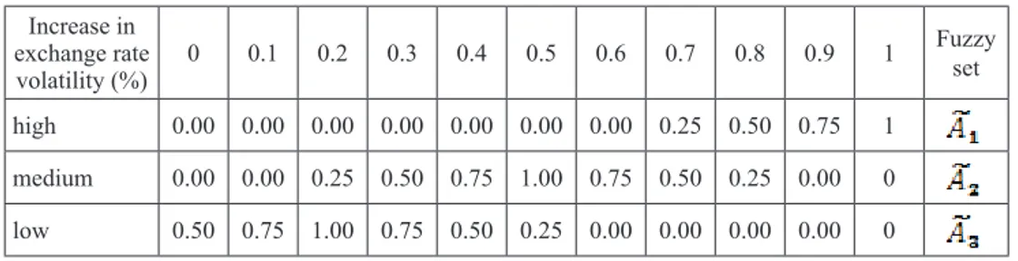
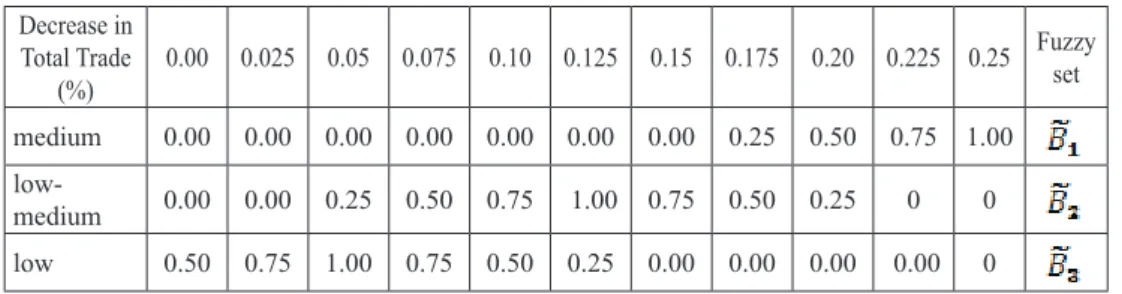
To start with, it is necessary to fuzzify exchange rate volatility and the decrease in bilateral trade. Describing process states by means of linguistic variables and using these variables as inputs is a very important step in the fuzzy approach. Table 2 shows the partitioning of the universe of exchange rate volatility into three fuzzy sets: ‘high’, ‘medium’ and ‘low’. Table 3 shows an analogous partitioning of the universe of total trade. When defi ning these expressions, membership values are assigned to each state intuitively based on experience (McNeill and Thro, 1994). A fuzzy set is defi ned solely by its membership function (Zimmermann, 2001). Membership degrees lie between 0 and 1. If an object completely belongs to the fuzzy set it has a membership value of 1. If an object does not belong to the fuzzy set at all, it has a membership value of 0. Membership degrees of borderline cases lie between 0 and 1. The more an element is characteristic of a fuzzy set, the closer to 1 is its membership degree (Driankov et al., 1996).
According to Table 2, “high increase in exchange rate volatility” is meant to be a 1% increase in volatility. If the increase is 0.9%, this volatility is considered to be high with a membership value of 0.75. When the volatility increases by 0.8%, the membership value for a high volatility decreases to 0.5. in Table 2 is the fuzzy set that describes a high increase in exchange rate volatility. Furthermore, a 0.5% increase in exchange rate volatility is defi ned as being medium and therefore it is assigned a membership value of 1 in , which is a fuzzy set that describes a medium increase in exchange rate volatility. Similarly, represents the fuzzy set that describes a low increase in exchange rate volatility. These three fuzzy sets are fully described by their membership functions. In fuzzy language, “high”, “medium” and “low” (increase in exchange rate volatility) are called linguistic values. “A” in general is the linguistic variable that represents “exchange rate volatility”.
On the other hand, , and are the fuzzy sets that describe a “medium”, “low-medium” and “low” decrease in total trade respectively. “B” in general is the linguistic variable that stands for “total trade”.
Table 2: Increase in exchange rate volatility partitioning
Increase in exchange rate
volatility (%)
0 0.1 0.2 0.3 0.4 0.5 0.6 0.7 0.8 0.9 1 Fuzzy
set
high 0.00 0.00 0.00 0.00 0.00 0.00 0.00 0.25 0.50 0.75 1
medium 0.00 0.00 0.25 0.50 0.75 1.00 0.75 0.50 0.25 0.00 0
low 0.50 0.75 1.00 0.75 0.50 0.25 0.00 0.00 0.00 0.00 0
Table 3: Decrease in total trade partitioning
Decrease in Total Trade
(%)
0.00 0.025 0.05 0.075 0.10 0.125 0.15 0.175 0.20 0.225 0.25 Fuzzy set medium 0.00 0.00 0.00 0.00 0.00 0.00 0.00 0.25 0.50 0.75 1.00
low-medium 0.00 0.00 0.25 0.50 0.75 1.00 0.75 0.50 0.25 0 0
low 0.50 0.75 1.00 0.75 0.50 0.25 0.00 0.00 0.00 0.00 0
Source: Authors`own description
We note the basic concepts of fuzzy set theory. A number is not necessarily high or low with a 100% certainty. If a value is closer to the target, its membership value is closer to 1. For example, in Table 2, a 0.7% increase in exchange rate volatility is categorized as a high increase with a 0.25 membership degree, while it is classifi ed as a medium increase with a membership value of 0.5. The membership degree to the fuzzy set is higher than because 0.7% is closer to 0.5% than it is to 1%. By contrast, in crisp sets, variables are categorized into specifi c classes, and they can only belong to one class. If a number belongs to one class, it cannot be member of another.
In this study, triangular membership functions are used due to computational effi ciency (Figure 1). Alternative often used functions are the trapezoidal and the bell-shaped functions. The triangular membership function
is defi ned by Driankov et al. (1996) as follows6:
⎪ ⎪ ⎩ ⎪ ⎪ ⎨ ⎧ > ≤ ≤ − − ≤ ≤ − − < = Λ γ γ β β γ γ β α α β α α γ β α u u u u u u u for 0 for ) /( ) ( for ) /( ) ( for 0 ) , , ; ( (5)
Figure 1: An example of a triangular function
1
α
β γSource: Driankov et al. (1996)
Figures 2 and 3 show the partitioning of the universe of exchange rate volatility and that of total trade into three fuzzy sets. These fi gures depict the information given in Tables 2 and 3 respectively. The linguistic variable “exchange rate volatility” in Figure 2 is described via 3 linguistic values which are “high”, “medium” and “low” increase in exchange rate volatility. Similarly, in Figure 3 the linguistic variable is “total trade” and linguistic values for it are “medium”, “low-medium” and “low” decrease in total trade.
Figure 2:Linguistic values for variable “exchange rate volatility”
0.2 0.4 0.5 0.6 0.8 1
1
μ Low Medium High
% change in volatility
0.1 0.3 0.7 0.9
0 0.5
Source: Authors`own drawing
Figure 3: Linguistic values for variable “total trade”
1
μ Low Low -Medium Medium
% change in total trade
0.5
0.05 0.1.0.125 0.15 0.2 0.25
0.025 0.075 0.175 0.225
0
When dealing with fuzzy sets, the entire knowledge of the system is stored as rules in the knowledge base (Zimmermann, 2001). Thus, the rules play a very important role in fuzzy systems and therefore a considerable effort should be taken when defi ning the rules. Detailed information on the problem to be solved and experience are necessary to design a reliable fuzzy rule set and to obtain good results. If the designer does not have suffi cient prior knowledge about the system or topic, it becomes impossible to develop a reliable fuzzy rule (Aliev et al., 2004). Fuzzy rules are the means that will translate inputs into the actual outputs (McNeill and Thro, 1994).
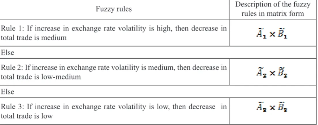
Under normal circumstances, traders do expect a stable economic environment and also no high volatility in exchange rates, as high volatility in exchange rates means high volatility in their revenues as well. When exchange rates fl uctuate a lot, the impact of this change on total trade will be considerable, as economic agents do not expect enormous changes in exchange rate volatility. The construction of the fuzzy rule used in this study follows the assumption that, while any increase in exchange rate volatility will affect total trade, the amount of decrease in total trade will not be exactly by the same percentage but lower. According to the fuzzy rule used (see Table 4), a high increase in exchange rate volatility (1 percent) results in a medium (0.25 percent) decrease in bilateral trade, while a medium (0.5 percent) increase in exchange rate volatility leads to a low-medium (0.125 percent) decrease in bilateral trade. Furthermore, a low increase in exchange rate volatility causes a low decrease in bilateral trade.
Table 4: Fuzzy rules for explaining the effects of increase in exchange rate volatility on bilateral trade
Fuzzy rules Description of the fuzzy
rules in matrix form Rule 1: If increase in exchange rate volatility is high, then decrease in
total trade is medium Else
Rule 2: If increase in exchange rate volatility is medium, then decrease in total trade is low-medium
Else
Rule 3: If increase in exchange rate volatility is low, then decrease in total trade is low
Source: Authors`own description
via linguistic values and quantitative values are assigned to these values. Then, possible consequences are defi ned for each possible input with ‘if-then’ rules (see Table 4), and the consequences are aggregated into a fuzzy set (see Figure 4). The last step is defuzzifi cation, where one crisp value is generated from the fuzzy output set. The crisp value obtained after defuzzifi cation enables the interpretation of the effect of a “1% increase in exchange rate volatility” on bilateral trade as a percentage value. Figure 4 shows how the whole process works.
Figure 4: The process of fuzzifi cation and defuzzifi cation
Fuzzy Rules
Fuzzification Computational
Unit Defuzzification
Input Output
Fuzzy World Crisp World
Source: Reconstructed from Zimmermann (2001) and Driankov et al. (1996)
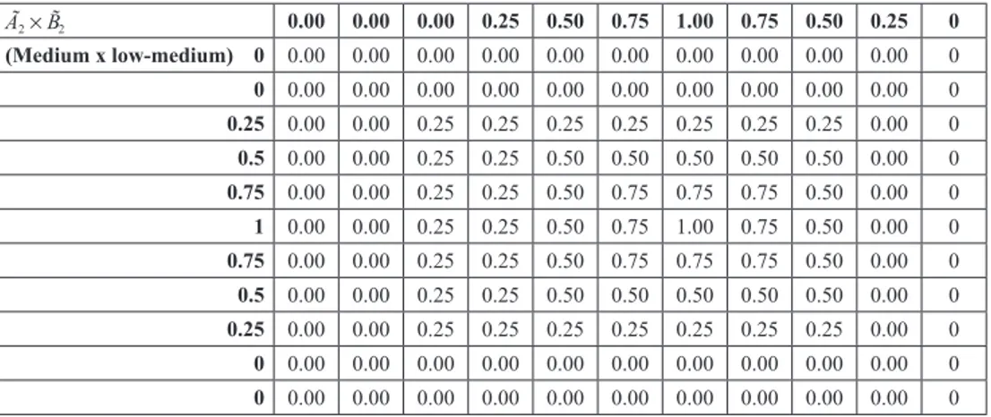
Given the conclusions obtained by individual fuzzy rules shown in Table 4, the overall fuzzy relation ( ) is calculated by taking the union of all individual effects:
(6)
where and are fuzzy sets and “x” denotes the Cartesian product. The Cartesian product of and shows the impact of a high increase in exchange rate volatility on bilateral trade in a matrix form. Similarly, and depict the effect of a medium and a low increase in exchange ra te volatility on bilateral trade respectively, again in a matrix form. The combination of these three individual effects is obtained by applying the union operator to these three matrices and the resultant matrix is . Using this fuzzy relation ( ) in matrix form, the impact of a “1 percent increase in exchange rate volatility” on bilateral trade will be determined (See Section 3.2.4 for fuzzy mathematics used and Appendix for the calculation of
To determine this effect we need to fuzzify “1% increase in exchange rate volatility”. The fuzzy set , called “1% increase in exchange rate volatility”, is described by the membership function illustrated in Figure 57.
Figure 5: Membership function for a “1% increase in volatility”
μ 1
0.5
% increase in volatility 1
0.8 0.6
Source: Authors`own drawing
According to this membership function, a 1% increase in exchange rate volatility has a membership value of 1 to the fuzzy set . When the increase in exchange rate volatility is nearer to 1%, for example 0.9%, its membership value is 0.75. A 0.8% increase in exchange rate volatility is the member of the fuzzy set of “1% increase in exchange rate volatility” with a degree of 0.5.
The effect of a 1 percent increase in exchange rate volatility on bilateral trade can be obtained by applying the compositional rule of inference to the fuzzy set and fuzzy relation : (see A.4 Defi nition 6 for details about the compositional rule of inference and operator “ ”).
,
where C˜ = [0 0 0 0 0 0 0 0.25 0.5 0.75 1] as shown in Figure 5.
is the fuzzifi ed decrease in bilateral trade, where each number is a weight factor between 0 and 1, corresponding to the percentage values between 0 and 1 with an increment of 0.025 (see Table 3).
The last step requires the defuzzifi cation process, which converts the overall fuzzy conclusion ( ) into a real number that represents the decrease in bilateral
7 Although it appears that the membership function of “1% increase in exchange rate volatility”
trade following a 1% increase in exchange rate volatility. There are different defuzzifi cation methods. Here, the centroid method—the center of the output membership function–is employed in the defuzzifi cation process. This method uses a weighted average. Mathematically, it corresponds to the expected value of probability (Zimmermann, 2001). The centroid method yields that:
0x0+ 0.025 x0+0.05 x0.25+ 0.075 x0.25+ 0.1x0.25+ 0.12 5x0. 25+ 0.15 x0.25+ 0.175x0.25+ 0.2x0.5+ 0.225 x0.75+0.25 x1
0 + 0 + 0 .25 +0. 25 + 0. 25 + 0.2 5 + 0. 25 + 0.2 5 + 0.5 + 0.75 + 1
= 0.183 % Change =
In words, this means that a 1 percent increase in exchange rate volatility leads to a 0.18 percent decrease in bilateral trade. It is evident that this result is in accordance with the coeffi cient of 0.21 that was obtained by using panel data analysis with period fi xed effects and is reported in Table 1.
5. Conclusion
The results prove the hypothesis that the fuzzy logic can approximate the effects of exchange rate volatility on trade fl ows and it can be used as a complement to statistical models. This paper contributes to international economics literature with the robustness check it made. On the one hand, it analyzes bilateral trade fl ows using a large data set and obtains results in line with the literature. On the other hand, it uses a totally different approach to analyze the same issue. It is quite reasonable to make this robustness check in a case where we have suffi cient data to see what can be done in the absence of adequate data. In this study, the interest focuses especially on the effects of exchange rate volatility on bilateral trade fl ows. Therefore, only the effects of exchange rate volatility on trade fl ows are compared using two different approaches.
References
Akhtar M.A. and R.S. Hilton (1984) “Effects of Exchange Rate Uncertainty on German and US Trade”, Federal Reserve Bank of NewYork Quarterly Review
9(1), pp. 7-16.
Aliev R. A. et al. (2004) Soft Computing and its Applications in Business and Economics, Springer Verlag: Berlin Heidelberg.
Baccheta P., van Wincoop E. (2000) “Does Exchange Rate Stability Increase Trade and Welfare?”, The American Economic Review 90(5), pp. 1093-1108.
Benčina J. (2007) “The use of fuzzy logic in coordinating investment projects”, Zbornik radova Ekonomskog fakulteta u Rijeci 25 (1), pp. 113-140.
Bubula A., Otker-Robe I. (2003) “Are Pegged and Intermediate Exchange Rate Regimes More Crisis Prone?”, IMF Working Paper.
Cushman D. O. (1983) “The Effects of Real Exchange Rate Risk on International Trade”, Journal of International Economics 15(1), pp. 45-63.
De Grauwe P., de Bellefroid B. (1987) “Long run exchange rate variability and international trade”, In: Arndt S., Richardson J.D. (Eds.), Real Financial Linkages Among Open Economies, London: MIT Press.
Driankov D. et al. (1996) An Introduction to Fuzzy Control, Berlin-Heidelberg-NewYork: Springer.
Ethier W. (1973) “International Trade and the Forward Exchange Market”,
American Economic Review 63(3), pp. 494-503.
Fischer S. (2001) “Distinguished Lecture on Economics in Government: Exchange Rate Regimes: Is the Bipolar View Correct?”, The Journal of Economic Perspectives 15(2), pp. 3-24.
Fu K.-S., Yao J. T. P. (1980) “Application of Fuzzy Sets in Earthquake Engineering”,
Working Paper Purdue University.
Gotur P. (1985) “Effects of Exchange Rate Volatility on Trade”, IMF Staff Papers
32, pp. 475- 512.
Hsiao C. (2003) Analysis of Panel Data, Cambridge: Cambridge University Press. Hooper P., Kohlhagen S. W. (1978) “The effects of Exchange Rate Uncertainty
on the Prices and Volume of International Trade”, Journal of International Economics 8(4), pp. 483-511.
Huang R. R. (2007) “Distance and trade: disentangling unfamiliarity effects and transport cost effects”, European Economic Review 51, pp. 161-181.
International Monetary Fund (1984) “Exchange Rate Volatility and World Trade: A Study by the Research Department of the IMF”, Occasional Paper 28.
Kowalski P. (2006) The Impact of the Economic and Monetary Union in the EU on International Trade- A Reinvestigation of the Exchange Rate Volatility Channel, Ph.D Thesis, University of Sussex.
Krugman P. R., Obstfeld M. (2006) International Economics: Theory and Policy, London: Pearson Addison Wesley.
Lane P.R., Milesi-Ferretti G. M. (2002) “External Wealth, the Trade Balance and the Real Exchange Rate”, European Economic Review 46, pp. 1049-1071 Lee V. C.S., Wong H. T. (2007) “A Multivariate Neuro-fuzzy System for Foreign
Currency Risk Management Decision Making”, Neurocomputing 70, pp. 942-951. McNeill F. M., Thro E. (1994) Fuzzy Logic: A Practical Approach, London:
Academic Press Limited.
Oyuk E. et al. (2007)“The Impact of Exchange Rates on International Trade in Europe from 1960s till 2000 Using a Modifi ed Gravity Model and Fuzzy Approach”, In: Proceedings of the 9th International Symposium on Operations Research, 26–28 September, Nova Gorica, Slovenia, pp. 219-224.
Tseng F.-M. et al. (2001) “Fuzzy ARIMA Model for Forecasting the Foreign Exchange Market”, Fuzzy Sets and Systems 118, pp. 9-19.
Viane J.-M., de Vries C. G. (1992) “International Trade and Exchange Rate Volatility”, European Economic Review 36(6), pp. 1311-21.
Zadeh L. A. (1973) “Outline of a new approach to the analysis of complex systems and decision processes”, IEEE Transactions on Systems, Man and Cybernetics
3, pp. 28-44.
Zadeh L.A. (1975) “The concept of a linguistic variable and its application to approximate reasoning – I”, Information Science 8, pp. 199-249.
Utjecaj volatilnosti te
č
aja na me
đ
unarodne trgovinske tijekove
Elif Nuroğlu1, Robert M. Kunst2
Sažetak
Cilj ovog rada je analizirati utjecaj volatilnosti tečaja na međunarodne trgovinske tijekove pomoću dva različita pristupa i to panel analize podataka i fuzzy logike, te potom usporediti rezultate. Prema platformi presjeka dimenzija 91 par EU15 zemlje s vremenskim rasponom 1964–2003. godine primjenjuje se prošireni gravitacijski model trgovine kako bi se utvrdili utjecaji volatilnosti tečaja na bilateralne trgovinske tijekove u zemljama EU15. Procijenjeni utjecaj je jasno negativan, što znači da volatilnost tečaja ima negativan utjecaj na bilateralne trgovinske tijekove. Potom, ovaj tradicionalni platformni pristup je u suprotnosti s alternativnom istragom temeljenom na fuzzy pristupu. Ključni elementi fuzzy pristupa su intuitivno postaviti fuzzy pravila odlučivanja i dodijeliti funkcije članstva fuzzy skupovima temeljem iskustva. Vidljivo je da oba pristupa daju vrlo slične rezultate, te se fuzzy pristup preporuča kao dopuna postojećih statističkih metoda.
Ključne riječi: jezično modeliranje, fuzzy odnos, volatilnost tečaja, bilateralna trgovina, gravitacijski model
JEL klasifi kacija: C23, F14
1 Docentica, Internacionalno sveučilište u Sarajevu, Fakultet menadžmenta i javne uprave,
Hrasnička cesta 15, 71000 Sarajevo, Bosna i Hercegovina. Znanstveni interes: međunarodna trgovina, makroekonomija, trgovinski model gravitacije. Tel.: +387 33 957 407. Fax: +387 33 957 105. E-mail: [email protected]. Osobna web stranica: www.ius.edu.ba/enuroglu (kontakt osoba).
2 Redoviti profesor, Sveučilište u Beču, Odsjek ekonomije i Institut za napredne studije, Brünner
Appendix
Calculation of Overall Fuzzy Relation
Table 1: Calculation of the decrease in total trade according to the Fuzzy Rule 1 in Table 4
à 1 B̃1 0.00 0.00 0.00 0.00 0.00 0.00 0.00 0.25 0.50 0.75 1
(High x medium) 0 0.00 0.00 0.00 0.00 0.00 0.00 0.00 0.00 0.00 0.00 0
0 0.00 0.00 0.00 0.00 0.00 0.00 0.00 0.00 0.00 0.00 0
0 0.00 0.00 0.00 0.00 0.00 0.00 0.00 0.00 0.00 0.00 0
0 0.00 0.00 0.00 0.00 0.00 0.00 0.00 0.00 0.00 0.00 0
0 0.00 0.00 0.00 0.00 0.00 0.00 0.00 0.00 0.00 0.00 0
0 0.00 0.00 0.00 0.00 0.00 0.00 0.00 0.00 0.00 0.00 0
0 0.00 0.00 0.00 0.00 0.00 0.00 0.00 0.00 0.00 0.00 0
0.25 0.00 0.00 0.00 0.00 0.00 0.00 0.00 0.25 0.25 0.25 0.25
0.5 0.00 0.00 0.00 0.00 0.00 0.00 0.00 0.25 0.50 0.50 0.5
0.75 0.00 0.00 0.00 0.00 0.00 0.00 0.00 0.25 0.50 0.75 0.75
1 0.00 0.00 0.00 0.00 0.00 0.00 0.00 0.25 0.50 0.75 1 Source: Authors’ calculation according to the fuzzy rule described in Table 4
Table 2: Calculation of the decrease in total trade according to the Fuzzy Rule 2 in Table 4
à 2 B̃2 0.00 0.00 0.00 0.25 0.50 0.75 1.00 0.75 0.50 0.25 0
(Medium x low-medium) 0 0.00 0.00 0.00 0.00 0.00 0.00 0.00 0.00 0.00 0.00 0
0 0.00 0.00 0.00 0.00 0.00 0.00 0.00 0.00 0.00 0.00 0
0.25 0.00 0.00 0.25 0.25 0.25 0.25 0.25 0.25 0.25 0.00 0
0.5 0.00 0.00 0.25 0.25 0.50 0.50 0.50 0.50 0.50 0.00 0
0.75 0.00 0.00 0.25 0.25 0.50 0.75 0.75 0.75 0.50 0.00 0
1 0.00 0.00 0.25 0.25 0.50 0.75 1.00 0.75 0.50 0.00 0
0.75 0.00 0.00 0.25 0.25 0.50 0.75 0.75 0.75 0.50 0.00 0
0.5 0.00 0.00 0.25 0.25 0.50 0.50 0.50 0.50 0.50 0.00 0
0.25 0.00 0.00 0.25 0.25 0.25 0.25 0.25 0.25 0.25 0.00 0
0 0.00 0.00 0.00 0.00 0.00 0.00 0.00 0.00 0.00 0.00 0
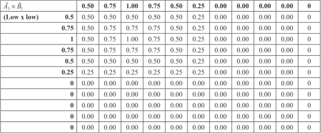
Table 3: Calculation of the decrease in total trade according to the Fuzzy Rule 3 in Table 4
à 3 B̃3 0.50 0.75 1.00 0.75 0.50 0.25 0.00 0.00 0.00 0.00 0
(Low x low) 0.5 0.50 0.50 0.50 0.50 0.50 0.25 0.00 0.00 0.00 0.00 0
0.75 0.50 0.75 0.75 0.75 0.50 0.25 0.00 0.00 0.00 0.00 0
1 0.50 0.75 1.00 0.75 0.50 0.25 0.00 0.00 0.00 0,00 0
0.75 0.50 0.75 0.75 0.75 0.50 0.25 0.00 0.00 0.00 0.00 0
0.5 0.50 0.50 0.50 0.50 0.50 0.25 0.00 0.00 0.00 0.00 0
0.25 0.25 0.25 0.25 0.25 0.25 0.25 0.00 0.00 0.00 0.00 0
0 0.00 0.00 0.00 0.00 0.00 0.00 0.00 0.00 0.00 0.00 0
0 0.00 0.00 0.00 0.00 0.00 0.00 0.00 0.00 0.00 0.00 0
0 0.00 0.00 0.00 0.00 0.00 0.00 0.00 0.00 0.00 0.00 0
0 0.00 0.00 0.00 0.00 0.00 0.00 0.00 0.00 0.00 0.00 0
0 0.00 0.00 0.00 0.00 0.00 0.00 0.00 0.00 0.00 0.00 0 Source: Authors’ calculation according to the fuzzy rule described in Table 4
Table 4: The overall fuzzy relation ( )
(R̃) 0.5 0.5 0.5 0.5 0.5 0.25 0.00 0.00 0.00 0.00 0.00
0.5 0.75 0.75 0.75 0.5 0.25 0.00 0.00 0.00 0.00 0.00
0.5 0.75 1 0.75 0.5 0.25 0.25 0.25 0.25 0.00 0.00
0.5 0.75 0.75 0.75 0.5 0.5 0.5 0.5 0.25 0.00 0.00
0.5 0.5 0.5 0.5 0.75 0.75 0.75 0.5 0.25 0.00 0.00
0.25 0.25 0.25 0.5 0.75 1 0.75 0.5 0.25 0.00 0.00
0.00 0.00 0.25 0.5 0.75 0.75 0.75 0.5 0.25 0.00 0.00
0.00 0.00 0.25 0.5 0.5 0.5 0.5 0.5 0.25 0.25 0.25
0.00 0.00 0.25 0.25 0.25 0.25 0.25 0.25 0.5 0.5 0.5
0.00 0.00 0.00 0.00 0.00 0.00 0.00 0.25 0.5 0.75 0.75
0.00 0.00 0.00 0.00 0.00 0.00 0.00 0.25 0.5 0.75 1