School of Economics and Management

(1)

Carlos Pestana Barros & Nicolas Peypoch

A Comparative Analysis of Productivity Change in Italian and Portuguese Airports

WP 006/2007/DE _________________________________________________________

António Afonso and Sebastian Hauptmeier

Fiscal Behaviour in the European Union: Rules, Fiscal Decentralization and Government Indebtedness

WP 23/2009/DE/UECE _________________________________________________________

Department of Economics

WORKING PAPERS

ISSN Nº0874-4548

School of Economics and Management

(2)

Fiscal behaviour in the European Union: rules,

fiscal decentralization and government

indebtedness

*

António Afonso

$ #

and Sebastian Hauptmeier

$

March 2009

Abstract

We assess the fiscal behaviour in the European Union countries for the period 1990-2005 via the responsiveness of budget balances to several determinants. The results show that the existence of effective fiscal rules, the degree of public spending decentralization, and the electoral cycle can impinge on the country’s fiscal position. Furthermore, the results also support the responsiveness of primary balances to government indebtedness.

JEL: C23, E62, H62

Keywords: fiscal regimes, fiscal rules, fiscal decentralization, European Union, panel data

*

We are grateful to Davide Furceri, Geert Langenus, Ad van Riet, Jürgen von Hagen, participants at the Public Finance Workshop Impact of Decentralization on Public Finances, Banque de France, Saint Germain en Laye, 2008, for helpful comments. The opinions expressed herein are those of the authors and do not necessarily reflect those of the ECB or the Eurosystem.

$

European Central Bank, Directorate General Economics, Kaiserstraße 29, D-60311 Frankfurt am Main, Germany, emails: antonio.afonso@ecb.europa.eu, sebastian.haupmeier@ecb.europa.eu.

#

(3)

Contents

Non-technical summary...3

1. Introduction ...4

2. Motivation and empirical strategy...5

2.1. The relevance of fiscal rules ...8

2.2. The degree of government spending decentralization...9

2.3. The relevance of the electoral cycle...10

3. Empirical analysis ...12

3.1. Primary balance reaction functions ...12

3.2. Primary spending reaction functions...15

4. Conclusion ...18

References ...19

Appendix A – Panel unit root results...32

(4)

Non-technical summary

In this paper we employ panel data analysis to assess the determinants of government’s fiscal behaviour for the 27 EU countries for the period between 1990 and 2005. We contribute to the literature by using, in the empirical analysis of government’s fiscal behaviour, both a set of fiscal rules and a government decentralisation measure among the determinants of fiscal discipline. For instance, we assess whether a higher degree of government spending decentralization is detrimental for a country’s fiscal position, a hypothesis that is corroborated by our empirical analysis.

Considering that cross-country dependence can mirror common changes in the behaviour of fiscal authorities (EU membership, run-up to EMU, SGP, peer pressure, capital markets views), that in recent years there is increased economic synchronization in the EU and that common policy shocks can affect fiscal positions in all EU countries, the use of a panel data approach seems therefore adequate. Moreover, the panel framework allows us to use the information contained in the cross-section dimension and increases the performance and accuracy of the estimated specifications. In addition, cross-country heterogeneity can also be captured by interaction terms, while variables may differ regarding their variances either on the cross-section or on the time series dimensions.

According to our results, the EU 27 governments increase the primary balance surplus as a result of increases in the outstanding stock of government debt. Both EMU and SGP arrangements have a statistically significant positive effect on the improvement of the fiscal position, which may imply an increased effort pursued by the EU countries to comply with the existing EU fiscal framework. On the other hand, we do not observe a statistically significant effect on primary spending. It is also possible to conclude that when the debt-to-GDP ratio is below the debt threshold of 80 percent a stronger overall fiscal rule contributes to improve the primary budget balance. Moreover, parliamentary elections negatively impinge on the improvement of the primary balance.

Regarding public spending decentralization, increasing the ratio of state plus local spending over central government spending contributes to an increase in the total primary spending-to-GDP ratio in the subsequent period, and when the debt ratio is above the 80 percent threshold we observe a more negative effect of the decentralisation proxy on primary balances. For instance, an increase of 1 percentage point of GDP in the decentralisation variable worsens the primary balance by 0.1 percentage points of GDP. Moreover, for a higher level of government indebtedness, the positive effect of spending decentralisation on primary spending is also higher.

(5)

1. Introduction

In the context of the European Union (EU), Member States face a fiscal

framework that asks for the implementation of sound fiscal policies, notably within the

Stability and Growth Pact (SGP) guidelines put forward in 1997. Such fiscal framework

is an indispensable tool for the well functioning of the European and Monetary Union

(EMU), which has been gradually put in place since 1992. However, the Member

States’ track records of complying with the fiscal rules laid down in the SGP have been

mixed. Therefore, it is relevant to assess what sort of determinants play a role in

contributing to the improvement of fiscal discipline in EU countries. Certainly, the

degree of national implementation and ownership of the European fiscal framework, i.e.

the existence of supportive and effective fiscal rules at the Member State level, seems to

be of high relevance in this context.

A recent study by the European Commission1 points to significant heterogeneity

of national fiscal frameworks within the European Union and suggests that ‘stronger’

fiscal rules indeed are conducive to sound public finances. Moreover, the study argues

that there seems to be a recent trend to stronger integration of sub-national levels of

government into the national rules framework, an aspect of particular importance in

countries like Germany or Spain which are characterised by a pronounced fiscal

federalism.2 In the absence of fiscal policy coordination at the mentioned level, a high

level of budget decentralisation, for example, might well interfere with the ability to

comply with national or European fiscal targets respectively. Further well-known

determinants of governments’ fiscal behaviour are the level of government

indebtedness, i.e. whether increases of primary surpluses occur as a response to higher

government debt ratios, as well as the relevance of electoral budget cycles.

1

See European Commission (2006).

2

(6)

Therefore, in this paper we employ panel data analysis to assess the

determinants of government’s fiscal behaviour for the 27 EU countries for the period

between 1990 and 2005. We contribute to the literature by using, in the empirical

analysis of government’s fiscal behaviour, both a set of fiscal rules and a government

decentralisation measure among the determinants of fiscal discipline. For instance, we

assess whether a higher degree of government spending decentralization is detrimental

for a country’s fiscal position, a hypothesis that is corroborated by our empirical

analysis.

Considering that cross-country dependence can mirror common changes in the

behaviour of fiscal authorities (EU membership, run-up to EMU, SGP, peer pressure,

capital markets views), that in recent years there is increased economic synchronization

in the EU and that common policy shocks can affect fiscal positions in all EU countries,

the use of a panel data approach seems therefore adequate. Moreover, the panel

framework allows us to use the information contained in the cross-section dimension

and increases the performance and accuracy of the estimated specifications. In addition,

cross-country heterogeneity can also be captured by interaction terms, while variables

may differ regarding their variances either on the cross-section or on the time series

dimensions.

The paper is organised as follows. Section Two provides motivation and

describes the empirical strategy. Section Three presents and discusses our results.

Section Four summarises the paper’s main findings.

2. Motivation and empirical strategy

When thinking about the determinants of fiscal behaviour it seems pertinent to

(7)

the existing stock of general government debt. The underlying idea being that if fiscal

authorities are driven by debt stabilization and sustainability motives, a positive

response of budget balances to the stock of outstanding government debt should be

expected. Therefore, a fiscal policy reaction function where a measure of the primary

balance reacts to the debt variable is a possible avenue for such analysis:

1 1 1

it i it it it it it it

s =

β

+

δ

s ₋ +

θ

b ₋ +

λ

z ₋ +

φ

f +

γ

x +

α

t +u . (1)

In (1) the index i (i=1,…,N) denotes the country, the index t (t=1,…,T) indicates

the period and βi stands for the individual effects to be estimated for each country i. sit is

the primary balance as a percentage of GDP for country i in period t, sit-1 is the

observation on the same series for the same country i in the previous period, and bit-1 is

the debt-to-GDP ratio in period t-1 for country i. z is the output gap, computed as the

difference between actual GDP and potential GDP as a percentage of potential GDP

and, f is a fiscal rule indicator, and x is a vector of additional institutional, political, and

other control variables such as the degree of public spending decentralization, and

specific dummy variables to signal EU enlargement, the run-up phase to EMU and SGP

sub-periods. Additionally, it is assumed that the disturbances uit are independent across

countries and time fixed effects are also included.

The use of primary rather than total balances is justified by the fact that the

intertemporal government budget constraint relates to the primary surplus. Moreover,

the use of the primary balance is logical since primary expenditure is more easily under

the discretionary control of the government. Under such a fiscal reaction function, one

assumes that the primary balance of period t is dependent on last year’s primary

balance. Hence, making the primary balance a function of government debt, allows

testing, for instance, if θ > 0, in other words, if the government tries to increase the

(8)

the government budget constraint, which could be seen as a sign that primary surpluses

positively reacting to government indebtedness.3 In other words, in such a regime,

primary budget balances are expected to react to government debt, in order to ensure

fiscal solvency.

The use of a panel framework, apart from allowing the use of the information

contained in the cross-section dimension, also increases the performance and accuracy

of the estimated specifications. In addition, one should point out that although the

variance of the decentralisation measure is more cross-sectional, the variance of

government indebtedness is both cross-sectional and time series related.

There are some econometric issues that come up when estimating equation (1).

Since our panel has a relatively small time dimension (16 years) with respect to the

number of units in the panel (27countries), it then important to check for the absence of

a bias related to the dynamic specification. In particular, if the Least Square Dummy

Variable estimator (LSDV) is used to estimate a dynamic model, results may suffer

from the well-known “Nickell-Bias” (see Nickell, 1981). While a number of consistent

Instrumental Variables (IV) and General Method of Moments (GMM) estimators4 have

been proposed to deal with this issue in micro panels characterised by a large number of

cross-sectional units, Monte Carlo evidence points to the superiority of bias corrected

LSDV estimators (LSDVC) in relatively narrow macro panels. Among others, Judson

and Owen (1999) present simulation results showing that when N is small bias-corrected

LSDV estimators outperform IV-GMM estimators both in terms of bias and root mean

squared. Therefore, we estimate equation (1) using a LSDVC estimator proposed by

Bruno (2005) which is also suitable for unbalanced panels.

3

See, for instance, Afonso (2008a) for additional discussions and results on this issue, while Favero (2002) also reports that fiscal policy reacts to increases in debt.

4

(9)

2.1. The relevance of fiscal rules

As one of the determinants of fiscal behaviour we also used several fiscal rule

indicators, as described by Ayuso-i-Casals at al. (2007) and EC (2006), which try to

model national numerical fiscal rules in the EU countries from 1990 to 2005. Fiscal

rules played a relevant role during the fiscal consolidations in the latter part of the

1990s.5 Well defined and targeted fiscal rules may help in promoting fiscal

consolidation and can help attain and safeguard a sustainable fiscal position. Such

indicators can be considered as part of the vector x of institutional and other control

variables in (1), and can include, for instance, deficit rules or expenditure rules.

According to Ayuso-i-Casals et al. (2007) there seems to be a link between

numerical rules and budgetary outcomes, with an increase in the share of government

finances covered by numerical fiscal rules leading to lower deficits. Moreover, they also

argue that countries where numerical fiscal rules are designed in such a way as not to

hamper the stabilisation function of fiscal policy the fiscal stance appears to behave

more counter-cyclically. Debrun and Kumar (2007) and Debrun et al. (2008) also report

that stricter and broader fiscal rules are associated with higher cyclically adjusted

primary balances and that lower cyclically adjusted primary balances are also observed

in election years. Wierts (2008) reports empirical evidence that expenditure rules can

limit to some extent the expenditure bias. Additionally, Pina and Venes (2007) provide

evidence that expenditure rules are associated to more prudent budget balance forecast

errors.

5

(10)

2.2. The degree of government spending decentralization

Another piece of information that may influence how successful the fiscal

authorities are in determining fiscal policy can be the degree of government fiscal

decentralization existing in a given country. The most common gauge for measuring

fiscal decentralisation is the sub-national share of government spending and revenue,

which varies considerably across countries.6

For instance, one could think that in a more centralised country, where most of

the government spending occurs at the central government level, may perhaps be less

difficult to reign in the budget deficit. In other words, in more decentralised institutional

fiscal settings, the less significant could be the responses and improvements in the

primary balance, since the coordination/control of the sectors/entities responsible for the

final spending actions can be more difficult.7 Nevertheless, one should be aware that

even if data are available regarding the structure of spending within the general

government sub-sectors, the mandate to spend may still be allocated at the central level,

but such information is then rather difficult to assess empirically.

To assess the validity of the hypothesis that decentralisation at the spending

level matters for fiscal behaviour, naturally linked to the existence and importance of

sub-national government levels, we have built an indicator of government spending

decentralisation, dec. This indicator is based on the general government sub-sectors

classifications and is computed as the sum of government spending from the state

(StateG), regional and local governments (RegLocG) sub-sectors over central (CenG),

state, regional and local government spending, therefore, excluding social security

6

See, for instance, OECD (2003).

7

(11)

spending. Indeed, we should consider the social security funds sub-sector as providing

an overall service that is not directly linked to the spending decisions of the other

sub-sectors of the general government. Therefore, we have, for country i in period t:

decit=(StateGit + RegLocGit)/(CenGit+ StateGit + RegLocGit ), (2)

which is computed with data from Eurostat. 8 In addition, we will also use a so-called

revenue decentralization measure, computed as in (2), both for total revenues and for

the sum of direct and indirect taxes.

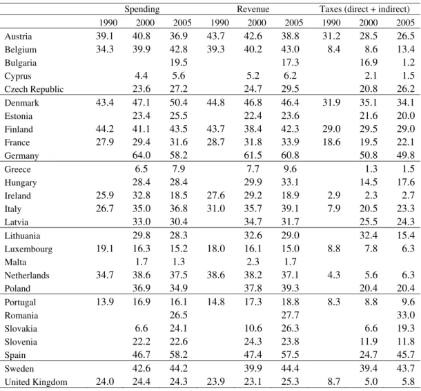
Table 1 illustrates the share of government spending, government revenue and

tax revenue, ascribed to each sub-national government. For instance, it is possible to

observe that the decentralisation of government spending was above 50 percent in 2005

for Spain, Germany and Denmark, while being below 20 percent for Ireland, Portugal or

Greece.

[Table 1]

From an empirical perspective, the indicator of government spending

decentralization can be interacted either with the government debt-to-GDP ratio or with

the fiscal rule indicator. This can provide additional insight on how such variable

influences overall government fiscal behaviour.

2.3. The relevance of the electoral cycle

The differences in government’s behaviour, which take into account the

electoral cycle, are predicted and discussed by the literature on the relations between

elections and fiscal performance, which can be traced back to Nordhaus (1975) and

8

(12)

Hibbs (1977), respectively regarding opportunistic and partisan cycles.9 We assess the

influence of the electoral budget cycle on fiscal behaviour by using a dummy

variable, E it

D , defined as

1, if in country there were elections for the parliament in 0, otherwise

E it

i t

D = ⎨⎧

⎩ . (3)

In order to test the relevance of the electoral cycle, the fiscal policy reaction

function can be amended to include an interaction term between, for instance, b and the

dummy variable for the elections,

1 1 1 2(1 ) 1 1

E E

it i it it it it it it it it it

s = β +δs ₋ +θ D b ₋ +θ − D b ₋ +λz ₋ +φ f +γ x +u . (4)

The hypothesis to be tested is whether when there is an election governments

choose to deliver a more expansionary fiscal policy, therefore allowing for a more

mitigated response of the primary balance to increases in the government debt. In other

words, if indeed electoral budget cycles play a role in the government’s fiscal decisions.

For instance, Afonso (2008a) reports results for the period 1970-2003 showing

that the EU-15 governments have a tendency to use the primary budget surplus to

reduce the public debt-to-GDP ratio. This response seems to be higher the higher is the

level of government indebtedness while governments also seem to improve the primary

budget balance as a result of increases in the outstanding stock of government debt.

Additionally, the results reported by Afonso (2008a) also indicate that primary balances

react positively and in a statistically significant way to government debt, when there are

no parliamentary elections in the next period, but this is not the overall case if there are

elections.

9

(13)

3. Empirical analysis

3.1. Primary balance reaction functions

Our data set is mostly taken from the European Commission Ameco database.

Since we are also interested in assessing the relevance of the existence of fiscal rules,

the data availability for this variable essentially restrains the time series dimension of

our panel to the period 1990-2005.10 We consider the 27 countries of the European

Union at that end of the period under analysis, even if some countries can be excluded

in some specifications due to missing data for some variables, which means we estimate

a dynamic unbalanced panel specification.11 The panel unit root test results, reported in

Appendix A, reveal that the null unit root hypothesis can be rejected at the ten per cent

level of significance for all or most of the cases, thus supporting the stationarity of our

fiscal variables and of the output gap.

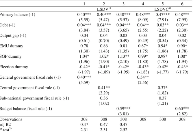
Table 2 presents the results for the baseline fiscal reaction function, drawing on

specification (1) for the primary balance, using the (corrected) least square dummy

variable estimator.12 It is possible to observe that the primary balance reaction to

government debt is statistically different from zero and positive, i.e. θ>0. In other

words, the EU 27 governments seem to act in accordance with the existing stock of

government debt, by increasing the primary balance surplus as a result of increases in

the outstanding stock of government debt. This is consistent with the prevalence of a

10

The data for the fiscal rules were provided by Ayuso-i-Casals et al (2007), and were computed on the basis of the responses to a questionnaire sent by the European Commission to the EU Member States, in the context of the Economic Policy Committee Working Group on the Quality of Public Finances. Data on parliamentary elections were obtained from the following sources:

http://www.idea.int/vt/total_number_of_elections.cfm and http://electionresources.org/.

11

Belgium, Denmark, Germany, Greece, Spain , France, Ireland, Italy, Luxembourg, Netherlands, Austria, Portugal, Finland, Sweden, United Kingdom, Cyprus, Czech Republic, Estonia, Hungary, Latvia, Lithuania, Malta, Poland, Slovakia, and Slovenia.

12

(14)

fiscal regime, where the fiscal authorities respond in a “stabilising” manner by

increasing primary balances when the debt ratio increases.

[Table 2]

Still considering Table 2, the fiscal position also improves when the existing

general government fiscal rule is stronger, i.e. φ>0, and the same is true for the case of

the central and balanced budget fiscal rules. Interestingly, this effect is more absent for

the case of sub-national government fiscal rules (see regressions 2 and 5 in Table 2).

Moreover, results indicate that the existence of parliamentary elections negatively

impinge on the improvement of the fiscal position.

In order to assess the relevance of the run-up to EMU and the importance of the

SGP effect, we have included additional explanatory dummy variables in the baseline

regression. Therefore, the EMU dummy assumes the value one for EU15 countries

between 1994 and 1998, and zero otherwise; the SGP dummy takes the value one after

1997 for the countries that are (adhered) in (to) the EU, and zero otherwise. From Table

2, the results show that both the EMU (only in the LSDVC estimations) and the SGP

dummy variables have a statistically significant positive effect on the improvement of

the fiscal position, which may imply an increased effort pursued by the EU countries to

comply with the existing EU fiscal framework.

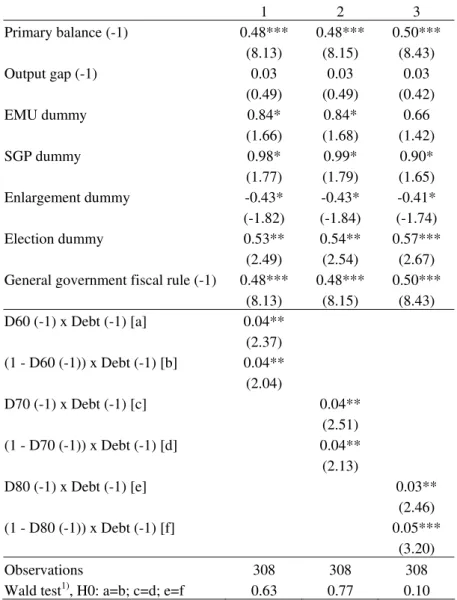
The relevance of government indebtedness can be further assessed using

interaction terms between the level of the debt-to-GDP ratio and alternative debt ratio

thresholds (60, 70, or 80 percent). In other words, the debt threshold dummy

variables, TH it

D , are defined as follows:

1, if debt ratio > T H , in country i in period t

, T H = 0.6, 0.7, 0.8 0, otherw ise

T H it

D = ⎨⎧

(15)

Table 3 provides the set of results with the above mentioned dummy variables,

and it is possible to observe that the responsiveness of the primary balance to

government debt is rather similar and only marginally lower when the debt-to-GDP

ratio is above the higher threshold. This could imply that the authorities find it more

difficult to increase primary surpluses when facing higher government debt ratios.

Interestingly, adding an enlargement dummy, which has the value one for the New

Member States after they join the EU, and zero otherwise, it is possible to capture a

decreasing effect on primary balances.

[Table 3]

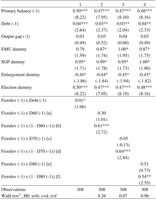
Taking advantage of the debt ratio threshold dummy variables defined in (5) we

can interact them with the overall fiscal rule at our disposal. The results reported in

Table 4 show that when the debt-to-GDP ratio is below the debt thresholds of 60, 70 or

80 percent a stronger overall fiscal rule contributes to improve the primary budget

balance (columns 2, 3 and 4 of Table 4). On the other hand, if the debt ratio is above the

aforementioned debt thresholds, the existence of the fiscal rule does not statistically

contribute to improve the fiscal behaviour of the government. Therefore, both lower

debt ratios and strong fiscal rules seem to be a good strategy for a better fiscal response

from primary balances. Interestingly, at the debt ratio threshold of 80 percent, the effect

of the overall fiscal rule comes out as less relevant for the improvement of the primary

balance. In addition, only for the debt ratio threshold of 70 per cent is the null

hypothesis of equal responses from the primary balance rejected.

[Table 4]

Table 5 reports the results regarding the analysis of whether government

spending decentralisation is relevant for fiscal behaviour using the decentralisation

(16)

[Table 5]

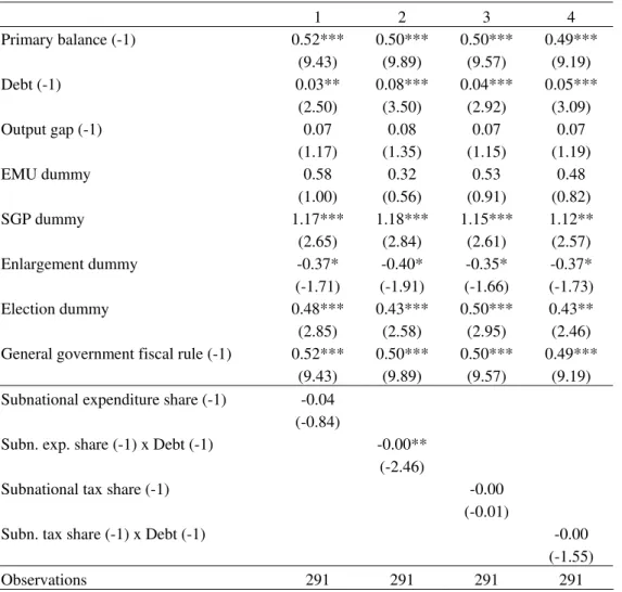
According to Table 5, a higher degree of government spending decentralisation

has a statistically significant negative effect on primary balances, when the

decentralisation variable is used together with the debt ratio. An increase in the

decentralisation variable (an increase in the share of non-central government spending

over total government spending, excluding social security funds) worsens the primary

balance. A similarly constructed tax decentralisation variable does not show up as

statistically significant.

3.2. Primary spending reaction functions

In order to complement our analysis, we also specify a fiscal policy reaction

function for primary spending, along the lines of the one used so far for the primary

balance:

1 1 2 1 3 1 4 5 6

it i it it it it it it

ps = w + w ps ₋ + w b ₋ + w z ₋ + w f + w x + w t +v , (6)

where ps is the primary spending-to-GDP ratio, and the other variables are similar to

what was already mentioned for the primary balance specification in (1). Additionally,

we now also include in the fiscal rule indicator, f, an expenditure rule. Tables 6 to 7

provide the set of results for the alternative estimation of the primary spending reaction

function (6). Again, we take account of a potential bias resulting from the dynamic

specification of our regression equation by using the bias corrected least square dummy

variable estimator.

[Table 6]

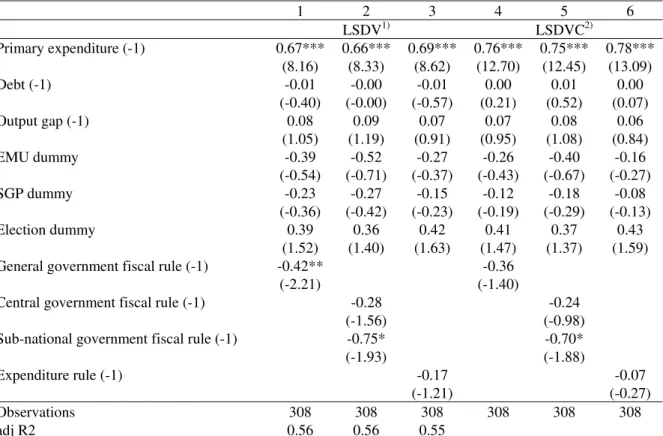
From Table 6 we see that the EMU and the SGP dummy variables, in contrast to

our results for the primary balance, do not affect primary spending significantly. The

(17)

expenditure, which, however, is only statistically significant if we perform standard

least square dummy variable estimation. When correcting for the dynamic panel bias the

effect turns insignificant. In contrast, the negative impact of fiscal rules at the

sub-national level turns out to be robust with regard to the estimation procedure. This

suggests a particular relevance of fiscal rules at the regional/local level for containing

general government spending. Interestingly, the expenditure rule is not statistically

significant, albeit the estimated coefficient has the right sign (columns 3 and 6 in Table

6). On the other hand, elections have the effect of rising primary spending, but this

effect is not statistically significant in all specifications.

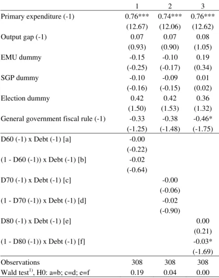
The interaction terms between the level of government indebtedness and the

debt ratio thresholds, reported in Table 7, show that when debt increases the

governments decrease primary spending in the next period but essentially if the debt

ratio is below the 80 percent threshold. This result is consistent with our previous

finding that governments were more able to improve their primary budget balances

when government indebtedness was below the debt thresholds.

[Table 7]

The results of the interaction between the overall general government fiscal rule

and the debt threshold dummy variables are reported in Table 8. In contrast to the case

of the primary balance reaction function, we do not observe that the level of debt

matters for the effectiveness of fiscal rules, regarding the effect on primary spending. In

addition, there is no evidence that the magnitude of the effect of the fiscal rule in

reducing primary spending is higher when the government indebtedness is beyond or

below a certain debt threshold.

(18)

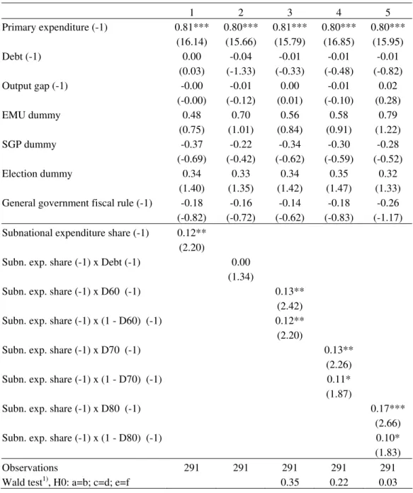
Turning now to the issue of spending decentralisation we observe from Table 9

that higher decentralisation increases primary spending, an effect that is mostly

statistically significant. In addition, it is possible to conclude that for very high levels of

government indebtedness (above 80% of GDP), the positive effect of spending

decentralisation on primary spending is also higher (see column 5 in Table 9).

Therefore, increasing (decreasing) the share of non-central (central) government

spending in total (minus social security) spending contributes to an increase in the total

primary spending-to-GDP ratio in the subsequent period.

[Table 9]

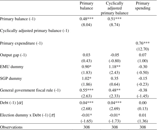
We also report in Table 10 the estimated specifications using the election

dummy variable, for the fiscal reaction function of primary balance, cyclically adjusted

primary balance, and primary spending. Note that we use an alternative version of the

election interaction in (4), in order to more easily discriminate the election effects, since

the estimated coefficients for the version in (4) are quite close. Thus, we estimated, for

instance, the following specification for the primary balance,

1 1

... E ...

it i it it it it

s =

α

+ +

α

b ₋ +

π

D b ₋ + + u , (7)

It is possible to observe, from (7) and from (4), that when there are no elections

(D_itE =0) we have α=θ2and when there are elections (DitE =1) we haveα+π=θ1.

[Table 10]

According to the results from Table 10 we can see, for instance, that the

improvement of the primary balance, as a response to the debt, decreases slightly when

an election occurs (π is negative and statistically significant). The same result is visible

for the cyclically adjusted primary balance. On the other hand, the consolidation effort

via the reduction of primary spending, as a result of an increase in the government

(19)

4. Conclusion

In this paper we estimated dynamic panel data specifications to assess the

determinants of government’s fiscal behaviour for the 27 EU countries for the period

between 1990 and 2005. Our analysis focussed on the responses, to several

determinants, of primary budget balances and primary spending.

According to our results, the EU 27 governments increase the primary balance

surplus as a result of increases in the outstanding stock of government debt. Both EMU

and SGP arrangements have a statistically significant positive effect on the

improvement of the fiscal position, which may imply an increased effort pursued by the

EU countries to comply with the existing EU fiscal framework. On the other hand, we

do not observe a statistically significant effect on primary spending. It is also possible to

conclude that when the debt-to-GDP ratio is below the debt threshold of 80 percent a

stronger overall fiscal rule contributes to improve the primary budget balance.

Moreover, parliamentary elections negatively impinge on the improvement of the

primary balance.

Regarding public spending decentralization, increasing the ratio of state plus

local spending over central government spending contributes to an increase in the total

primary spending-to-GDP ratio in the subsequent period, and when the debt ratio is

above the 80 percent threshold we observe a more negative effect of the decentralisation

proxy on primary balances. For instance, an increase of 1 percentage point of GDP in

the decentralisation variable worsens the primary balance by 0.1 percentage points of

GDP. Moreover, for a higher level of government indebtedness, the positive effect of

(20)

All in all, we can say that the existence of fiscal rules, a lower degree of public

spending decentralization positively contribute to a higher responsiveness of primary

surpluses to government indebtedness (a more Ricardian behaviour of the fiscal

authorities in the EU), while the electoral cycle also has the expected effect. In terms of

future work, one can think, for instance, of assessing other measures of fiscal

decentralization or alternative data regarding the proxy for fiscal rules.

References

Afonso, A. (2008a). “Ricardian Fiscal Regimes in the European Union”, Empirica, 35

(3), 313–334.

Afonso, A. (2008b). “Expansionary fiscal consolidations in Europe: new evidence”.

Applied Economics Letters, forthcoming, DOI

http://dx.doi.org/10.1080/13504850701719892.

Alesina, A. and Roubini, N. (1992). Political Business Cycles in OECD Economies,

Review of Economic Studies, 59 (4), 663-688.

Anderson, T. and Hsiao, C. (1981). “Estimation of Dynamic Models with Error

Components”, Journal of the American Statistical Association, 76, 598-606.

Andersson, B. and Minarik, J. (2008). “Design choices for fiscal policy rules”, in

Servaas, S. and Kastrop, C. (eds.) The quality of public finances. Findings of the

Economic Policy Committee-Working Group (2004-2007), European Economy −

Economy Paper No. 311 (Brussels: European Commission).

Arellano, M. and Bond, S.R. (1991). “Some Tests of Specification for Panel Data:

Monte Carlo Evidence and an Application to Employment Equations”, Review

of Economic Studies, 58, 277-297.

Ayuso-i-Casals, J.; Hernandez, D.; Moulin, L. and Turrini, A. (2007). “Beyond the

SGP: Features and effects of EU national-level fiscal rules”, mimeo, presented at the

Bank of Italy Workshop held in Perugia, 29-31 March 2007.

Blundell, R. and Bond, S. (1998). “Initial conditions and moment restrictions in

(21)

Breitung, J. (2000). “The Local Power of Some Unit Root Tests for Panel Data” in

Baltagi, B. (ed.), Nonstationary Panels, Panel Cointegration, and Dynamic Panels.

Advances in Econometrics, Vol. 15. Amsterdam: JAI.

Bruno, G. (2005). “Approximating the bias of the LSDV estimator for dynamic

unbalanced panel data models”, Economic Letters, 87, 361–366.

Dában, T.; Detragiache, E.; di Bella, G.; Milesi-Ferretti, G. and Symansky, S. (2003).

“Rules-Based Fiscal Policy in France, Germany, Italy, and Spain”, IMF Occasional

Paper 225.

Debrun, X. and Kumar, M. (2007). “The Discipline-Enhancing Role of Fiscal

Institutions: Theory and Empirical Evidence”, IMF WP/07/171.

Debrun, X.; Moulin, L.; Turrini, A.; Ayuso-i-Casals, J and Kumar, M. (2008). “Tied to

the mast? National fiscal rules in the European Union”, Economic Policy, 23 (54),

297–362.

European Commission (2006). “Public Finances in EMU,” European Economy, No 3,

2006.

Favero, C. (2002). “How do Monetary and Fiscal Authorities Behave?” CEPR

Discussion Paper 3426.

von Hagen, J. and Eichengreen, B. (1996). “Federalism, Fiscal Restraints, and European

Monetary Union”, American Economic Review, 86 (2), 134-138.

Hibbs, D. (1977). “Political Parties and Macroeconomic Policy”, American Political

Science Review. 7, 1467-1487.

Hauptmeier, S.; Heipertz, M. and Schuknecht, L. (2007). “Expenditure reform in

industrialised countries: a case study approach”, Fiscal Studies, 28 (3), 293-342.

Im, K., Pesaran, M. and Shin, Y. (2003). “Testing for Unit Roots in Heterogeneous

Panels”, Journal of Econometrics, 115 (1), 53-74.

Judson, R. and Owen, A. (1999). “Estimating dynamic panel data models: a guide for

macroeconomists”, Economics Letters, 65, 9-15.

Levin, A., Lin, C.-F. and Chu, C.-S. (2002). “Unit Root Tests in Panel Data:

Asymptotic and Finite Sample Properties”, Journal of Econometrics, 108 (1), 1-24.

Maddala, G. and Wu, S. (1999). “A Comparative Study of Unit Root Tests and a New

Simple Test”, Oxford Bulletin of Economics and Statistics, 61 (1), 631-652.

Nickell, S. (1981). "Biases in Dynamic Models with Fixed Effects", Econometrica, 49,

(22)

Nordhaus, W. (1975). “The Political Business Cycle”, Review of Economic Studies. 42,

169-190.

Oates, W. (1999). “An essay on fiscal federalism”, Journal of Economic Literature, 37,

1120-1149.

OECD (2003). “Fiscal relations across levels of government”, OECD Economic

Outlook 74, December, 143-160.

Pina, A. and Venes, N. (2007). “The political economy of EDP fiscal forecasts: an

empirical assessment”, ISEG/UTL Department of Economics, Working Paper

023/2007/DE/UECE.

Stegarescu, D. (2005). “Public Sector Decentralisation: Measurement Concepts and

Recent International Trends”. Fiscal Studies, 26 (3), 301–333

Rogoff, K. and Sibert, A. (1988). Elections and Macroeconomic Policy Cycles, Review

of Economic Studies, 55 (1), 1-16.

Wierts, P. (2008). “How do expenditure rules affect fiscal behaviour?” DNB Working

(23)

Table 1 – Share of sub-national spending/revenue in government spending/revenue (State + Local)/(Central+ State + Local), %

Spending Revenue Taxes (direct + indirect) 1990 2000 2005 1990 2000 2005 1990 2000 2005 Austria 39.1 40.8 36.9 43.7 42.6 38.8 31.2 28.5 26.5

Belgium 34.3 39.9 42.8 39.3 40.2 43.0 8.4 8.6 13.4

Bulgaria 19.5 17.3 16.9 1.2

Cyprus 4.4 5.6 5.2 6.2 2.1 1.5

Czech Republic 23.6 27.2 24.7 29.5 20.8 26.2

Denmark 43.4 47.1 50.4 44.8 46.8 46.4 31.9 35.1 34.1

Estonia 23.4 25.5 22.4 23.6 21.6 20.0

Finland 44.2 41.1 43.5 43.7 38.4 42.3 29.0 29.5 29.0

France 27.9 29.4 31.6 28.7 31.8 33.9 18.6 19.5 22.1

Germany 64.0 58.2 61.5 60.8 50.8 49.8

Greece 6.5 7.9 7.7 9.6 1.3 1.5

Hungary 28.4 28.4 29.9 33.1 14.5 17.6

Ireland 25.9 32.8 18.5 27.6 29.2 18.9 2.9 2.3 2.7

Italy 26.7 35.0 36.8 31.0 35.7 39.1 7.9 20.5 23.3

Latvia 33.0 30.4 34.7 31.7 25.5 24.3

Lithuania 29.8 28.3 32.6 29.0 32.4 15.4

Luxembourg 19.1 16.3 15.2 18.0 16.1 15.0 8.8 7.8 6.3

Malta 1.7 1.3 2.3 1.7

Netherlands 34.7 38.6 37.5 38.6 38.2 37.1 4.3 5.6 6.3

Poland 36.9 34.9 37.8 39.3 20.4 20.4

Portugal 13.9 16.9 16.1 14.8 17.3 18.8 8.3 8.8 9.6

Romania 26.5 27.7 33.0

Slovakia 6.6 24.1 10.6 26.3 6.6 19.3

Slovenia 22.2 22.6 24.3 23.8 11.9 11.8

Spain 46.7 58.2 47.4 57.5 24.7 45.7

Sweden 42.6 44.2 39.9 44.4 39.4 43.7

United Kingdom 24.0 24.4 24.3 23.9 23.1 25.3 8.7 5.0 5.8

(24)

Table 2 – Fiscal reaction function for the primary balance (fixed-effects, 1990-2005)

Notes: The t (z) statistics are in parentheses in specifications 1-3 (4-6).

*, **, *** - statistically significant at the 10, 5, and 1 percent level respectively. EMU dummy, 1 for EU15 countries between 1994 and 1998, 0 otherwise. SGP dummy, 1 after 1997 for the countries that are (adhered) in (to) the EU, 0 otherwise.

1) _{Standard least square dummy variable estimator.}

2) _{Bias corrected least square dummy variable estimator proposed by Bruno (2005).}

3) _{F-statistic tests for fixed effects,}_{H0: fixed effects jointly insignificant.}_{F(24,262)-values reported, 1% critical} value = 1.83.

1 2 3 4 5 6

LSDV1) LSDVC2)

Primary balance (-1) 0.40*** 0.40*** 0.40*** 0.48*** 0.47*** 0.48*** (5.59) (5.47) (5.57) (8.09) (7.91) (7.95)

Debt (-1) 0.04*** 0.04*** 0.04*** 0.04** 0.03** 0.03**

(3.84) (3.57) (3.65) (2.55) (2.22) (2.30)

Output gap (-1) 0.04 0.04 0.03 0.03 0.04 0.02

(0.61) (0.70) (0.49) (0.49) (0.54) (0.34)

EMU dummy 0.78 0.86 0.81 0.87* 0.94* 0.90*

(1.30) (1.43) (1.35) (1.75) (1.86) (1.78)

SGP dummy 1.04* 1.02* 1.13** 0.99* 0.98* 1.08*

(1.96) (1.90) (2.10) (1.80) (1.78) (1.94)

Election dummy -0.42* -0.41* -0.42* -0.43* -0.42* -0.43*

(-1.97) (-1.89) (-1.95) (-1.83) (-1.77) (-1.79) General government fiscal rule (-1) 0.40*** 0.54**

(5.59) (2.56)

Central government fiscal rule (-1) 0.41** 0.37*

(2.29) (1.82)

Sub-national government fiscal rule (-1) 0.36 0.37

(1.02) (1.21)

Budget balance fiscal rule (-1) 0.59*** 0.60***

(3.81) (2.82)

Observations 308 308 308 308 308 308

adj R2 0.47 0.47 0.47

(25)

Table 3 – Fiscal reaction function for the primary balance (fixed-effects, 1990-2005), the relevance of debt thresholds (LSDVC)

1 2 3 Primary balance (-1) 0.48*** 0.48*** 0.50***

(8.13) (8.15) (8.43)

Output gap (-1) 0.03 0.03 0.03

(0.49) (0.49) (0.42)

EMU dummy 0.84* 0.84* 0.66

(1.66) (1.68) (1.42)

SGP dummy 0.98* 0.99* 0.90*

(1.77) (1.79) (1.65)

Enlargement dummy -0.43* -0.43* -0.41*

(-1.82) (-1.84) (-1.74)

Election dummy 0.53** 0.54** 0.57***

(2.49) (2.54) (2.67) General government fiscal rule (-1) 0.48*** 0.48*** 0.50***

(8.13) (8.15) (8.43)

D60 (-1) x Debt (-1) [a] 0.04**

(2.37) (1 - D60 (-1)) x Debt (-1) [b] 0.04**

(2.04)

D70 (-1) x Debt (-1) [c] 0.04**

(2.51) (1 - D70 (-1)) x Debt (-1) [d] 0.04**

(2.13)

D80 (-1) x Debt (-1) [e] 0.03**

(2.46)

(1 - D80 (-1)) x Debt (-1) [f] 0.05***

(3.20)

Observations 308 308 308

Wald test1)_{, H0: a=b; c=d; e=f} _0.63 _0.77 _0.10

Notes: The z statistics are in parentheses.

(26)

Table 4 – Fiscal reaction function for the primary balance (fixed-effects, 1990-2005), the relevance of fiscal rules (LSDVC)

1 2 3 4

Primary balance (-1) 0.50*** 0.47*** 0.47*** 0.48***

(8.22) (7.95) (8.10) (8.16)

Debt (-1) 0.04*** 0.03** 0.03** 0.04**

(2.64) (2.37) (2.04) (2.33)

Output gap (-1) 0.03 0.03 0.04 0.03

(0.49) (0.52) (0.60) (0.49)

EMU dummy 0.79 0.87* 1.00* 0.87*

(1.59) (1.74) (1.95) (1.75)

SGP dummy 0.95* 0.99* 0.95* 1.00*

(1.71) (1.78) (1.73) (1.80)

Enlargement dummy -0.44* -0.44* -0.45* -0.43*

(-1.86) (-1.84) (-1.94) (-1.82)

Election dummy 0.50*** 0.47*** 0.47*** 0.48***

(8.22) (7.95) (8.10) (8.16)

Fisrulov (-1) x Debt (-1) 0.01*

(1.66) Fisrulov (-1) x D60 (-1) [a] 0.30

(1.01)

Fisrulov (-1) x (1 - D60 (-1)) [b] 0.61***

(2.72)

Fisrulov (-1) x D70 (-1) [c] -0.05

(-0.13) Fisrulov (-1) x (1 - D70 (-1)) [d] 0.64***

(2.84)

Fisrulov (-1) x D80 (-1) [e] 0.51

(0.73)

Fisrulov (-1) x (1 - D80 (-1)) [f] 0.54**

(2.55)

Observations 308 308 308 308

Wald test1), H0: a=b; c=d; e=f 0.26 0.07 0.96

*, **, *** - statistically significant at the 10, 5, and 1 percent level respectively. EMU dummy, 1 for EU15 countries between 1994 and 1998, 0 otherwise. SGP dummy, 1 after 1997 for the countries that are (adhered) in (to) the EU, 0 otherwise. Enlargement dummy, 1 for the New Member States after entering the EU, 0 otherwise.

(27)

Table 5 – Fiscal reaction function for the primary balance (fixed-effects, 1990-2005), the relevance of government spending and revenue decentralisation (LSDVC)

1 2 3 4 Primary balance (-1) 0.52*** 0.50*** 0.50*** 0.49***

(9.43) (9.89) (9.57) (9.19)

Debt (-1) 0.03** 0.08*** 0.04*** 0.05***

(2.50) (3.50) (2.92) (3.09)

Output gap (-1) 0.07 0.08 0.07 0.07

(1.17) (1.35) (1.15) (1.19)

EMU dummy 0.58 0.32 0.53 0.48

(1.00) (0.56) (0.91) (0.82)

SGP dummy 1.17*** 1.18*** 1.15*** 1.12**

(2.65) (2.84) (2.61) (2.57)

Enlargement dummy -0.37* -0.40* -0.35* -0.37*

(-1.71) (-1.91) (-1.66) (-1.73)

Election dummy 0.48*** 0.43*** 0.50*** 0.43**

(2.85) (2.58) (2.95) (2.46) General government fiscal rule (-1) 0.52*** 0.50*** 0.50*** 0.49***

(9.43) (9.89) (9.57) (9.19)

Subnational expenditure share (-1) -0.04

(-0.84)

Subn. exp. share (-1) x Debt (-1) -0.00**

(-2.46)

Subnational tax share (-1) -0.00

(-0.01)

Subn. tax share (-1) x Debt (-1) -0.00

(-1.55)

(28)

Table 6 – Fiscal reaction function for the primary spending (fixed-effects, 1990-2005)

Notes: The t (z) statistics are in parentheses in specifications 1-3 (4-6).

1) Standard least square dummy variable estimator.

2) Bias corrected least square dummy variable estimator proposed by Bruno (2005).

1 2 3 4 5 6

LSDV1) LSDVC2)

Primary expenditure (-1) 0.67*** 0.66*** 0.69*** 0.76*** 0.75*** 0.78*** (8.16) (8.33) (8.62) (12.70) (12.45) (13.09)

Debt (-1) -0.01 -0.00 -0.01 0.00 0.01 0.00

(-0.40) (-0.00) (-0.57) (0.21) (0.52) (0.07)

Output gap (-1) 0.08 0.09 0.07 0.07 0.08 0.06

(1.05) (1.19) (0.91) (0.95) (1.08) (0.84)

EMU dummy -0.39 -0.52 -0.27 -0.26 -0.40 -0.16

(-0.54) (-0.71) (-0.37) (-0.43) (-0.67) (-0.27)

SGP dummy -0.23 -0.27 -0.15 -0.12 -0.18 -0.08

(-0.36) (-0.42) (-0.23) (-0.19) (-0.29) (-0.13)

Election dummy 0.39 0.36 0.42 0.41 0.37 0.43

(1.52) (1.40) (1.63) (1.47) (1.37) (1.59) General government fiscal rule (-1) -0.42** -0.36

(-2.21) (-1.40)

Central government fiscal rule (-1) -0.28 -0.24

(-1.56) (-0.98)

Sub-national government fiscal rule (-1) -0.75* -0.70*

(-1.93) (-1.88)

Expenditure rule (-1) -0.17 -0.07

(-1.21) (-0.27)

Observations 308 308 308 308 308 308

(29)

Table 7 – Fiscal reaction function for the primary spending (fixed-effects, 1990-2005), the relevance of debt thresholds (LSDVC)

1 2 3

Primary expenditure (-1) 0.76*** 0.74*** 0.76***

(12.67) (12.06) (12.62)

Output gap (-1) 0.07 0.07 0.08

(0.93) (0.90) (1.05)

EMU dummy -0.15 -0.10 0.19

(-0.25) (-0.17) (0.34)

SGP dummy -0.10 -0.09 0.01

(-0.16) (-0.15) (0.02)

Election dummy 0.42 0.42 0.36

(1.50) (1.53) (1.32)

General government fiscal rule (-1) -0.33 -0.38 -0.46*

(-1.25) (-1.48) (-1.75)

D60 (-1) x Debt (-1) [a] -0.00

(-0.22) (1 - D60 (-1)) x Debt (-1) [b] -0.02

(-0.64)

D70 (-1) x Debt (-1) [c] -0.00

(-0.06) (1 - D70 (-1)) x Debt (-1) [d] -0.02

(-0.90)

D80 (-1) x Debt (-1) [e] 0.00

(0.21)

(1 - D80 (-1)) x Debt (-1) [f] -0.03*

(-1.69)

(30)

Table 8 – Fiscal reaction function for the primary spending (fixed-effects, 1990-2005), the relevance of fiscal rules (LSDVC)

1 2 3 4

Primary expenditure (-1) 0.76*** 0.76*** 0.76*** 0.76*** (12.92) (12.79) (13.13) (12.92)

Debt (-1) 0.00 0.00 0.00 -0.00

(0.02) (0.19) (0.26) (-0.04)

Output gap (-1) 0.07 0.07 0.07 0.07

(0.98) (0.96) (0.94) (0.97)

EMU dummy -0.24 -0.25 -0.27 -0.21

(-0.39) (-0.41) (-0.43) (-0.33)

SGP dummy -0.14 -0.12 -0.10 -0.12

(-0.21) (-0.19) (-0.16) (-0.18)

Election dummy 0.40 0.40 0.41 0.40

(1.46) (1.46) (1.50) (1.45)

Fisrulov (-1) x Debt (-1) -0.01

(-1.47) Fisrulov (-1) x D60 (-1)[a] -0.44

(-1.25)

Fisrulov (-1) x (1 - D60 (-1)) [b] -0.35

(-1.26)

Fisrulov (-1) x D70 (-1) [c] -0.26

(-0.58)

Fisrulov (-1) x (1 - D70 (-1)) [d] -0.38

(-1.36)

Fisrulov (-1) x D80 (-1) [e] -0.98

(-1.13)

Fisrulov (-1) x (1 - D80 (-1)) [f] -0.36

(-1.37)

Wald test1), H0: a=b; c=d; e=f 0.79 0.81 0.46 0.79

(31)

Table 9 – Fiscal reaction function for the primary spending (fixed-effects, 1990-2005), the relevance of government spending decentralisation (LSDVC)

1 2 3 4 5 Primary expenditure (-1) 0.81*** 0.80*** 0.81*** 0.80*** 0.80***

(16.14) (15.66) (15.79) (16.85) (15.95)

Debt (-1) 0.00 -0.04 -0.01 -0.01 -0.01

(0.03) (-1.33) (-0.33) (-0.48) (-0.82)

Output gap (-1) -0.00 -0.01 0.00 -0.01 0.02

(-0.00) (-0.12) (0.01) (-0.10) (0.28)

EMU dummy 0.48 0.70 0.56 0.58 0.79

(0.75) (1.01) (0.84) (0.91) (1.22)

SGP dummy -0.37 -0.22 -0.34 -0.30 -0.28

(-0.69) (-0.42) (-0.62) (-0.59) (-0.52)

Election dummy 0.34 0.33 0.34 0.35 0.32

(1.40) (1.35) (1.42) (1.47) (1.33) General government fiscal rule (-1) -0.18 -0.16 -0.14 -0.18 -0.26

(-0.82) (-0.72) (-0.62) (-0.83) (-1.17) Subnational expenditure share (-1) 0.12**

(2.20)

Subn. exp. share (-1) x Debt (-1) 0.00

(1.34)

Subn. exp. share (-1) x D60 (-1) 0.13**

(2.42)

Subn. exp. share (-1) x (1 - D60) (-1) 0.12**

(2.20)

Subn. exp. share (-1) x D70 (-1) 0.13**

(2.26)

Subn. exp. share (-1) x (1 - D70) (-1) 0.11*

(1.87)

Subn. exp. share (-1) x D80 (-1) 0.17***

(2.66)

Subn. exp. share (-1) x (1 - D80) (-1) 0.10*

(1.83)

Observations 291 291 291 291 291

(32)

Table 10 – Fiscal reaction functions (fixed-effects, 1990-2005), the relevance of elections (LSDVC)

Primary balance

Cyclically adjusted primary balance

Primary spending

Primary balance (-1) 0.48*** 0.51***

(8.04) (8.74)

Cyclically adjusted primary balance (-1)

Primary expenditure (-1) 0.76***

(12.70)

Output gap (-1) 0.03 -0.05 0.07

(0.43) (-0.80) (1.00)

EMU dummy 0.90* 1.18** -0.30

(1.83) (2.43) (-0.50)

SGP dummy 1.02* 0.35 -0.15

(1.86) (0.64) (-0.23)

General government fiscal rule (-1) 0.55*** 0.48** -0.38

(2.63) (2.33) (-1.45)

Debt (-1) [α] 0.04*** 0.04*** 0.00

(2.68) (2.69) (0.13)

Election dummy x Debt (-1) [π] -0.01* -0.01* 0.01

(-1.65) (-1.73) (1.36)

(33)

Appendix A – Panel unit root results

The test proposed by Im, Pesaran and Shin (2003) has been widely implemented in

empirical research due to its rather simple methodology and alternative hypothesis of

heterogeneity. This test assumes cross-sectional independence among panel units

(except for common time effects), but allows for heterogeneity in the form of individual

deterministic effects (constant and/or linear time trend), and heterogeneous serial

correlation structure of the error terms. We also provide the results of four other panel

unit root tests: Levin, Lin and Chu (2002), Breitung (2000), and Fisher-type tests using

ADF and PP tests (Maddala and Wu, 1999). The results reveal that the null unit root

hypothesis can be rejected at the ten per cent level of significance for all or most of the

cases, thus supporting the stationarity of our fiscal variables and of the output gap.

Table A1 – Summary of panel data unit root tests for the primary balance (1989-2007)

Method Statistic P-value* Cross-sections Obs

Null: Unit root (assumes common unit root process)

Levin, Lin & Chu t stat -2.96244 0.0015 27 382

Breitung t-stat -3.83851 0.0001 27 355

Null: Unit root (assumes individual unit root process)

Im, Pesaran and Shin W-stat -3.33215 0.0004 27 382

ADF - Fisher Chi-square 90.1764 0.0015 27 382

PP - Fisher Chi-square 139.209 0.0000 27 409

* Probabilities for Fisher tests are computed using an asymptotic Chi-square distribution. All other tests assume asymptotic normality.

Automatic selection of lags based on SIC. Newey-West bandwidth selection using a Bartlett kernel

Table A2 – Summary of panel data unit root tests for the cyclically adjusted primary balance (1989-2007)

Breitung t-stat -2.50251 0.0062 27 335

(34)

Table A3 – Summary of panel data unit root tests for primary spending (1989-2007)

Breitung t-stat -0.72843 0.2332 27 340

Table A4 – Summary of panel data unit root tests for government debt (1989-2007)

Breitung t-stat 1.17238 0.8795 27 347

PP - Fisher Chi-square -4.71615 0.0000 27 374

Table A5 – Summary of panel data unit root tests for the output gap (1989-2007)

Breitung t-stat -2.66883 0.0038 27 358

(35)

Appendix B – OLS results

Table B1 – Fiscal reaction function for the primary balance (fixed-effects, 1990-2005)

1 2 3

Primary balance (-1) 0.47 *** 0.46 *** 0.47 ***

6.56 6.31 6.55

Debt (-1) 0.05 *** 0.04 *** 0.05 ***

4.17 3.98 4.07

Output gap (-1) 0.08 0.08 0.08

1.29 1.31 1.22

EMU dummy 0.70 *** 0.77 *** 0.75 ***

3.21 3.57 3.49

SGP dummy 0.47 * 0.56 ** 0.55 **

1.84 2.27 2.23

Enlargement dummy 0.33 0.24 0.28

0.74 0.54 0.64

Election dummy -0.52 ** -0.51 ** -0.52 **

-2.40 -2.34 -2.40

General government fiscal rule (-1) 0.37 ** - -

2.36

Central government fiscal rule (-1) - 0.35 * - 1.85 Sub-national government fiscal rule (-1) - 0.17 -

0.50

Budget balance fiscal rule (-1) - - 0.39 **

2.41

adj R2 0.71 0.71 0.71

Notes: The t statistics are in parentheses.

(36)

Table B2 – Fiscal reaction function for the primary balance (fixed-effects, 1990-2005), the relevance of debt thresholds

1 2 3

Primary balance (-1) 0.47 *** 0.47 *** 0.48 ***

6.52 6.50 6.47

Debt (-1) - - -

Output gap (-1) 0.08 0.08 0.08

1.29 1.29 1.17

EMU dummy 0.69 *** 0.65 *** 0.55 **

3.19 2.91 2.39

SGP dummy 0.47 * 0.37 0.36

1.83 1.32 1.35

Enlargement dummy 0.33 0.42 0.32 *

0.74 0.91 0.72

Election dummy -0.52 ** -0.53 ** -0.49 **

-2.41 -2.41 -2.25 General government fiscal rule (-1) 0.36 ** 0.36 ** 0.41 ***

2.29 2.34 2.62

D60 (-1) x Debt (-1) 0.05 *** - -

3.93

(1 - D60 (-1)) x Debt (-1) 0.05 *** - -

3.23

D70 (-1) x Debt (-1) - 0.05 *** -

4.21

(1 - D70 (-1)) x Debt (-1) - 0.06 *** -

3.71

D80 (-1) x Debt (-1) - - 0.05 ***

4.25

(1 - D80 (-1)) x Debt (-1) - - 0.07 ***

4.65

adj R2 0.71 0.71 0.72

(37)

Table B3 – Fiscal reaction function for the primary balance (fixed-effects, 1990-2005), the relevance of fiscal rules

1 2 3 4

Primary balance (-1) 0.48 *** 0.47 *** 0.46 *** 0.47 ***

6.67 6.51 6.49 6.47

Debt (-1) 0.05 0.05 *** 0.04 *** 0.05 ***

4.26 4.17 3.77 4.09

Output gap (-1) 0.08 0.08 0.08 0.08

1.18 1.29 1.34 1.29

EMU dummy 0.65 0.70 *** 0.83 *** 0.69 ***

2.94 3.20 3.67 3.09

SGP dummy 0.58 *** 0.48 * 0.47 * 0.47 *

2.22 1.84 1.82 1.80

Enlargement dummy 0.27 *** 0.32 0.28 0.33

0.62 0.72 0.64 0.74

Election dummy -0.53 -0.52 ** -0.54 ** -0.52 **

-2.43 -2.41 -2.47 -2.4

Fisrulov (-1) x Debt (-1) 0.00 *** - - -

1.97

Fisrulov (-1) x D60 (-1) - 0.35 * - -

1.69

Fisrulov (-1) x (1 - D60 (-1)) - 0.37 ** - -

2.16

Fisrulov (-1) x D70 (-1) - -0.143 -

-0.55

Fisrulov (-1) x (1 - D70 (-1)) - - 0.46 *** -

2.71

Fisrulov (-1) x D80 (-1) - - - 0.51

1.06

Fisrulov (-1) x (1 - D80 (-1)) - - - 0.36 ***

2.33

adj R2 0.72 0.71 0.72 0.71

(38)

Table B4 – Fiscal reaction function for the primary balance (fixed-effects, 1990-2005), the relevance of government spending decentralisation

1 2 3 4 5

Primary balance (-1) 0.53 *** 0.51 *** 0.53 *** 0.53 *** 0.54 ***

8.14 7.21 8.12 8.09 8.05

Debt (-1) 0.04 *** 0.09 *** 0.04 *** 0.04 *** 0.05 ***

3.30 4.45 2.90 3.30 3.72

Output gap (-1) 0.09 0.10 0.09 0.09 0.08

1.42 1.45 1.41 1.42 1.21

EMU dummy 0.81 *** 0.88 *** 0.81 *** 0.80 *** 0.68 ***

3.97 4.31 3.97 3.88 3.07

SGP dummy 0.73 *** 0.90 *** 0.73 *** 0.67 ** 0.64 **

2.69 3.16 2.64 2.37 2.30

Enlargement dummy 0.17 -0.20 0.17 0.19 0.17

0.39 -0.43 0.38 0.44 0.39

Election dummy -0.51 ** -0.52 ** -0.51 ** -0.52 ** -0.50 **

-2.41 -2.43 -2.41 -2.42 -2.33

General government fiscal rule (-1) 0.31 ** 0.26 * 0.31 ** 0.30 * 0.34 **

2.02 1.75 1.98 1.95 2.20

Subnational expenditure share (-1) -0.10 ** - - - -

-2.29

Subn. exp. share (-1) x Debt (-1) - 0.00 *** - - -

-2.99

Subn. exp. share (-1) x D60 (-1) - - -0.10 ** - -

-2.23

Subn. exp. share (-1) x (1 - D60) (-1) - - -0.10 ** - -

-2.28

Subn. exp. share (-1) x D70 (-1) - - - -0.10 ** -

-2.39

Subn. exp. share (-1) x (1 - D70) (-1) - - - -0.09 ** -

-2.06

Subn. exp. share (-1) x D80 (-1) - - - - -0.13 ***

-3.03

Subn. exp. share (-1) x (1 - D80) (-1) - - - - -0.09 **

-2.00

Observations 291 291 291 291 291

adj R2 0.76 0.76 0.76 0.76 0.76

(39)

Table B5 – Fiscal reaction function for the primary balance (fixed-effects, 1990-2005), the relevance of government tax decentralisation

1 2 3 4 5

Primary balance (-1) 0.51 *** 0.50 *** 0.51 *** 0.50 *** 0.51 ***

7.01 6.75 6.96 6.83 6.99

Debt (-1) 0.05 *** 0.06 *** 0.05 *** 0.05 *** 0.05 ***

4.03 4.58 3.79 4.16 4.22

Output gap (-1) 0.10 0.09 0.09 0.10 0.09

1.42 1.38 1.41 1.45 1.30

EMU dummy 0.84 *** 0.90 *** 0.85 *** 0.81 *** 0.78 ***

4.07 4.32 4.08 4.15 3.71

SGP dummy 0.62 ** 0.81 * 0.63 ** 0.60 ** 0.62 **

2.40 2.84 2.32 2.35 2.41

Enlargement dummy 0.07 -0.12 0.05 0.04 -0.03

0.45 -0.27 0.11 0.09 -0.07

Election dummy -0.49 ** -0.49 ** -0.49 ** -0.47 ** -0.50 **

-2.26 -2.31 -2.27 -2.18 -2.32

General government fiscal rule (-1) 0.29 * 0.25 0.29 * 0.29 * 0.27 *

1.93 1.63 1.84 1.78 1.76

Subnational tax share (-1) -0.03 - - - -

-1.17

Subn. tax share (-1) x Debt (-1) - 0.00 ** - - -

-2.11

Subn. tax share (-1) x D60 (-1) - - -0.03 - -

-1.06

Subn. tax share (-1) x (1 - D60) (-1) - - -0.03 - -

-1.18

Subn. tax share (-1) x D70 (-1) - - - -0.04 * -

-1.68

Subn. tax share (-1) x (1 - D70) (-1) - - - -0.02 -

-0.94

Subn. tax share (-1) x D80 (-1) - - - - -0.07 **

-2.15

Subn. tax share (-1) x (1 - D80) (-1) - - - - -0.01

0.75

Observations 291 291 291 291 291

adj R2 0.75 0.75 0.75 0.75 0.76

(40)

Table B6 – Fiscal reaction function for the primary spending (fixed-effects, 1990-2005)

1 2 3 4

Primary expenditure (-1) 0.67 *** 0.66 *** 0.68 *** 0.68 ***

8.23 8.31 8.54 8.44

Debt (-1) -0.01 -0.01 -0.01 -0.01

-0.89 -0.60 -0.87 -0.96

Output gap (-1) 0.05 0.06 0.06 0.06

0.72 0.80 0.82 0.76

EMU dummy -0.64 *** -0.71 *** -0.67 *** -0.63 ***

-2.63 -2.98 -2.77 -2.58

SGP dummy -0.38 -0.41 * -0.54 ** -0.57 **

-1.48 -1.75 -2.25 -2.13

Enlargement dummy 0.15 0.23 0.28 0.31

0.32 0.48 0.60 0.66

Election dummy 0.41 0.38 0.42 * 0.43 *

1.65 1.56 1.68 1.73

General government fiscal rule (-1) -0.35 * - - -

-2.01

Central government fiscal rule (-1) - -0.28 - -

-1.55

Sub-national government fiscal rule (-1) - -0.55 - -

-1.45

Budget balance fiscal rule (-1) - - -0.23 -

-1.32

Expenditure rule (-1) - - - -0.18

-1.22

adj R2 0.92 0.92 0.92 0.92

(41)

Table B7 – Fiscal reaction functions (fixed-effects, 1990-2005), the relevance of elections

Primary balance

Cyclically adjusted primary

balance

Primary spending

Primary balance (-1) 0.47*** - -

6.61 Cyclically adjusted primary balance (-1) - 0.47*** -

7.23

Primary expenditure (-1) - - 0.67***

8.27

Output gap (-1) 0.08 - 0.06

1.24 0.75

EMU dummy 0.70*** 0.45** -0.64***

3.21 2.07 -2.62

SGP dummy 0.46* -0.07 -0.36

1.78 -0.31 -1.43

Enlargement dummy 0.36 0.81* 0.13

0.81 1.83 0.27

General government fiscal rule (-1) 0.38** 0.42*** -0.36**

2.44 2.93 -2.07

Debt (-1) [α] 0.05*** 0.048*** -0.01

4.25 4.63 -0.98

Election dummy x Debt (-1) [π] -0.0068** -0.007** 0.006**

-2.38 -2.53 2.00

adj R2 0.71 0.74 0.92