Carlos Pestana Barros & Nicolas Peypoch
A Comparative Analysis of Productivity Change in Italian and Portuguese Airports
WP 006/2007/DE _________________________________________________________
Tanya Araújo and Gérard Weisbuch
The Labour Market on the Hypercube
WP 024/2007/DE/UECE _________________________________________________________
Departament of Economics
W
ORKINGP
APERSISSN Nº0874-4548
School of Economics and Management
The labour market on the hypercube
Tanya Ara´
ujo
ISEG, Universidade T´ecnica de Lisboa (TULisbon) and
Research Unit on Complexity in Economics (UECE)
email:tanya@iseg.utl.pt
G´erard Weisbuch
∗ ∗Laboratoire de Physique Statistique
∗de l’Ecole Normale Sup´erieure,
24 rue Lhomond, F-75231 Paris Cedex 5, France.
email:weisbuch@lps.ens.fr
October 9, 2007
Abstract
Positions offered on a labour market and workers preferences are here described by bit-strings representing individual traits. We study the co-evolution of workers and firm preferences modeled by such traits. Individual ”size-like” properties are controlled by binary en-counters which outcome depends upon a recognition process. De-pending upon the parameter set-up, mutual selection of workers and positions results in different types of attractors, either an exclusive niches regime or a competition regime.
PACS: 89.65.-s Social and economic systems
1
Introduction: hikers of the
hyper-cube
The study of dynamical systems most often concerns systems with few degrees of freedom, or spatial systems. Physicists are less concerned with other high dimensional systems. But many models in biology and the social sciences are based on bit strings of often large dimensions.
If we take the case of biology and especially genomics, the genome or the succession of monomers in biopolymers, is often represented by a bit string. This is e.g. the case for models of the origin of life [1], immunology [2], and of co-evolution [3].
These models are generally based on the following functional scheme:
Genome=⇒recognition=⇒action=⇒results=⇒population change.
The ”genome”, described by a bit string, undergoes selective en-counters with other genomes and some action with more or less suc-cessful results influences a death and/or ”birth” process.
These models also inspired social sciences: Cultural and opinion dynamics have been described by [4, 5]. The minority game [6] applies to finance. Finally the genetic algorithm approach [7] has a wide range of applications ranging from co-evolution to optimisation.
All these algorithms have in common the bit-string description and most often a recognition process, but they differ by the consequences of significant encounters, as stressed by the well known title in psy-chology: ”What do you do after your say Hello?”[8] .
Let us consider a set of job seekers looking for positions which characteristics are described by bit strings. We here simplify by con-sidering binary, independent characteristics.
The preferences of workersi depend upon the overlap qij of their
own ideal string, their requirement stringSi, with the position set of
characteristicsSj:
qij =Pkl=1Sil.EQ.Sjl (1)
Where the symbol EQ stands for the logical equivalence relation, which gives 1 if the two bits are equal and 0 otherwise. The recog-nition condition is that the overlap is larger than a fixed threshold. Encounters, position filling and generated profits (or losses) influence integrated continuous variables which control the persistence of the agents on the labour market. Our model, to be completely defined in the next section, then defines a co-evolution dynamics of workers and positions.
We are interested in the dynamics of population of agents on the string hypercube and in the stable patterns that may arise. We want to know how these patterns depend upon the parameters of the model: what are the different regimes, where are their transitions.
The model is based on a workers/positions co-evolution but it can also be applied to other domains, provided some degree of adjust-ments. One can think of other markets, such as production/consumption markets (as in [11]). In political science, one could model the co-evolution of political party platforms and voter choices as described by bit strings; each bit is now the position of the party (or the voter) on some specific issue, Europe, retirement policy, environment etc.
Such applications can be very concrete. A major car constructor can in principle provide a lot of options: their combination would correspond to more than ten thousands different cars. But not all combinations would sell well; furthermore each change on the produc-tion chain has a cost. The issue for the producers is which combinaproduc-tion of options should I propose to the public in view of its distribution of preferences. The same issue is faced by the local dealer: which stock of combinations should I keep available to the local public?
2
The Model
In the model there are Np firm agents and Nc worker agents. Each
are coded by a ”requirement” string of k bits. Each firm offers posi-tions which characteristics are also coded by a string of k bits. The bit string of a worker represents what the worker agent requests and the bit string of the firm is a code for the positionthat it proposes.
In addition to the two bit strings that code for requirements and position, the ”wealth” of each agent is defined by a scalar variableS
or C, depending upon the agent type (worker or firm, respectively). The variable Si represents the degree of satisfaction of the worker i
and Cj represents the capital accumulated by firmj.
In economy this role is played by money, but in other contexts it could be power or status.
The dynamics of the model is described by: Arecognition and position filling process.
At each time step, all workers look for positions closest to their requirements set (the position string with the largest overlap qij; in
the case of equality among several positions a random choice is made among them). If the relative overlap qij
k between the position and the
worker strings is larger than a thresholdθ, the position is filled by the worker whose satisfaction is changed according to:
Si(t+ 1) =Si(t)−ac+ qij
k (2)
Satisfaction is increased according the relative overlap of the require-ment and position strings. It is decreased by ac representing a
con-stant individual effort made by the worker. The satisfaction of those workers who don’t find accptable positions are simply decreased by
ac.
The equivalent updating of the firm capital is:
Cj(t+ 1) =Cj(t)−ap+Pi(j)qij
k (3)
Capital is increased by the set of filled positions during the time in-terval, according the relative overlaps of the requirement and position strings (workers productivity relates to the overlap). Capital is de-creased by a constant labour and investment cost ap.
APersistence and renewal process.
There is no upper limit to worker satisfaction or to firm capital. But due to the costs terms,ap and ac, they may decrease to zero.
A firm which capital would become negative quits the market and is not renewed.
initial satisfaction S0 and a randomly generated requirement string: we suppose that there exist different labour markets, say in different cities. Our model applies to the dynamics of one local market. Any unsatisfied worker moves to another city. The departures from our lo-cal market are balanced by influx of workers unsatisfied in other cities which look for new opportunities in the local market.
Both assumptions are simplifications. Firms might want to fill different kind of positions: we here assume that positions of a single kind are the most crucial for the survival of the firm. Firms might evolve by adaptation or new firms might appear on a given market. Adaptation is discussed in another report [11], but the present simpler model simply supposes that workers turnover and firm selection are faster processes than firm creation and adaptation.
3
Checking the parameter space
In principle there are eight independent parameters:
• The string lengthkand the thresholdθ for interaction.
• The constantsap and ac.
• The initial numbers of firms (Np) and workers (Nc).
• The initial endowments of firms (Cp) and workers (Sc).
In practice, because of the irreversibility of the firms removal pro-cess, Cp and Np influence mostly the early stages of the dynamics.
In terms of dynamical regimes and transitions, we might expect that the most important parameters are ac and θ (since we keep k
constant).
In equation 1, the positive term θk is between 0 and 1. Then, for large values ofac,aclarger than 1, the change in worker satisfaction is
negative. Workers dynamics is characterised by a renewal process of workers, with a rate of order Sc
ac: workers are created withS=Sc, and
their satisfaction can only linearly decrease to zero when they quit. On average their satisfaction is S = Sc/2. ac = 1 is then the critical
value of the satisfaction parameter separating the regime where some workers may increase their satisfaction with time and remain locally employed, from a renewal regime when all workers are condemned to nomadism across different labour markets.
ns(θ) which Hamming distance to the offered position string is less or
equal to k−θ. Any worker whose string is in the basin of satisfaction of a firm may interact and take the position. Fork= 10, θ= 1 gives a neighbourhood of size 1, size 11 for θ= 0.9, size 56 for θ= 0.8 etc. Comparingns(θ)×Npto 2k = 1024, the number of sites on the hyper-cube, gives an approximation of the condition in threshold separating the competition regime at low θ values, from the ”niche” regime. In the competition regime, workers may choose between different firms in their neighborhood; firms then compete for workers. In the niche regime, they are so far apart that they don’t compete.
In the competition regime, according to ap values, we might
pre-dict that competition will reduce a too large initial number of firms, until they get closer to the critical number where the niche regime is established. But according to initial conditions, essentiallyCpandNp,
the selection of surviving firms may end up in a variety of attractors as shown by simulations. Anyway, a maximum number of firms sur-viving on the local market in the competition regime can be estimated from equation 3. At equilibrium:
ap = NNcp<qkij>
Np= Napc<qkij>
(4)
These equations are based on an approximation of uniform distribu-tion of posidistribu-tion strings on the hypercube. On average each firm is surrounded by Nc
Np workers which contribute to its capital balance.
We will further observe that this upper bound is seldom reached.
4
Simulation results
Most simulations were made for a fixed set of parameters: String length k = 10, firms cost constant ap = 4.5, number of workers
(Nc=1000) and initial endowments of firms (Cp = 200) and
work-ers (Sc= 5). Simulation times were usually 2000, but we checked that
the stationary regime was reached by increasing simulation times up to 10000.
We studied the influence of workers effort constantac, thresholdθ
4.1
Time evolution
Let us first monitor the time evolution of firms capitalCi, of the
aver-age worker satisfaction S, of workers renewal rate and of the number of surviving firms.
0 500 1000 1500 2000
0 2000 4000 6000 8000
C
ap:4.5 ac:1 θ:0.9 Cp:200
0 500 1000 1500 2000
1.5 2 2.5 3 3.5 4 4.5 5
mean S
ac: 1
0 500 1000 1500 2000
0 200 400 600 800
Np:30 Nc:1000
workers renewal rate
0 500 1000 1500 2000
10 15 20 25 30
number of surviving firms
Figure 1: Time evolution of firms capital Ci, of the average worker
satisfac-tion S, of workers renewal rate and of the number of surviving firms. Np
initial was 30, Nc= 1000, ac= 1, Cp = 200, θ=.9.
In figure 1, whereNp initial was 30, Nc= 1000,ac= 1,θ=.9, we
see on the lower right curve that firms are first selected: there number is decreased from 30 to 11, and then business becomes profitable (C
evolution, on the upper left curves). The early firm selection gives figures much lower than the upper bound computed by equation 3 (which should be around 200), but surviving firms make profit.
Workers average satisfaction is always lower than 5: since ac = 1
reflects the division between a fraction f of condensed workers with
S = 5 and of unsatisfied workers with averageS= 2.5. f then obeys:
f×5 + (1−f)×2.5 =< S > (5)
f = < S >−2.5
2.5 (6)
The increase of< S >towards 5 with time then reflects the increase of the fraction of ”condensed” workers towards 1. This effect is confirmed by decrease of the renewal rate on the lower left plot.
0 500 1000 1500 2000
0 1000 2000 3000 4000
C
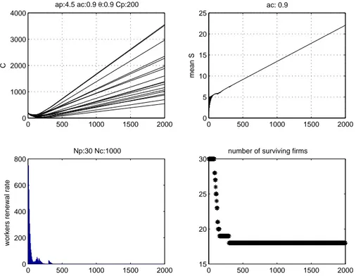
ap:4.5 ac:0.9 θ:0.9 Cp:200
0 500 1000 1500 2000
0 5 10 15 20 25
mean S
ac: 0.9
0 500 1000 1500 2000
0 200 400 600 800
Np:30 Nc:1000
workers renewal rate
0 500 1000 1500 2000
15 20 25 30
number of surviving firms
Figure 2: Time evolution of firms capital Ci, of the average worker
satis-faction S, of worker renewal rate and of the number of surviving firms. Np
initial was 30,Nc= 1000,θ =.9,Cp = 200, as on the previous figure but the
worker’s effort constant is now ac= 0.9 instead of 1.
With ac = 0.9, smaller than one, those condensed workers in the
lower stress on workers, they early find spots where they are able to survive, and they stabilize in the neighborhood of firms much earlier in time. The diversity of firms is higher: 17 survive.
4.2
Attractors
Let us now do a systematic study of the attractors of the dynamics. We checked the asymptotic state of the system through a similar set of variables: firms capitalCi, average worker satisfaction< S >, number
of surviving firms.
We also tried to characterise the degree of order or of diversity of the attractor configuration and used the overlap of workers require-ment strings as the order function. This is the same notion as used in spin glass theory. We then checked the fraction hh(10)(5) of the histogram of overlaps among workers requirement strings. This gives us an in-dication about how many workers are condensed and what is their repartition (even or uneven) in the neighborhood of firms.
In the next four figures, the horizontal variable is Np the initial
number of firms. The four sets of figures correspond to two values of
θ, 09 and 0.8, andac, 0.9 and 1. These results were averaged over 100
different random samplings of initial configurations.
There is not much to add about the influenceacfrom these figures.
But the influence ofθon the transition between a competition regime (θ=.8) and a niche regime (θ=.9) is now made clear.
In the niche regime,θ=.9, few firms survive, even for large initial numbers of firms (figure 3). Their number saturates around 20 for higher values of the initial firm number. Firms make a lot of profit (largeCvalues) (figure 4). Workers satisfaction depends uponac
(fig-ure 5). Significant values of h(10), corresponding mostly to workers which requirement string is exactly a seller position string, are ob-served when acand θ are both large.
On figure 6, the large value of the 10 overlap bin observed when
ac= 1 and θ=.9 is an indication that many workers have the same
requirement string. This concentration of requirement strings, co-occurring with small number of surviving firms, is obviously due to their ”condensation” on firms position strings. Furthermore, the large overlap value of 0.2 observed for ac = 1 and θ = 0.9 tells us that
their distribution among different firms is uneven; an even distribution would correspond to the inverse number of surviving firms, 0.05.
101 102 0
50 100 150
θ=0.8 ac=1
<Suv>
101 102
0 50 100 150
θ=0.8 ac=0.9
<Suv>
101 102
10 15 20 25
θ=0.9 ac=1
<Suv>
101 102
10 15 20 25
θ=0.9 ac=.9
<Suv>
Figure 3: Number of surviving firms. These are taken at time=2000. Np, the
initial number of firms is varied along the x axis (logarithmic scale). Each of the four plots correspond to a given pair of ac andθ values, upper plots to a
101 102 0
2000 4000 6000 8000 10000
θ=0.8 ac=1
<C>
101 102
0 2000 4000 6000 8000 10000
θ=0.8 ac=0.9
<C>
101 102
2000 4000 6000 8000 10000
θ=0.9 ac=1
<C>
101 102
0 2000 4000 6000 8000 10000
θ=0.9 ac=.9
<C>
Figure 4: Averaged firm capital Ci at time=2000. Np is varied along the x
axis (logarithmic scale). Each of the four plots correspond to a given pair of
101 102 4.2
4.4 4.6 4.8 5
θ=0.8 ac=1
<S>
101 102
20 25 30 35 40
θ=0.8 ac=0.9
<S>
101 102
4.7 4.75 4.8 4.85 4.9 4.95 5
θ=0.9 ac=1
<S>
101 102
20 25 30 35 40
θ=0.9 ac=.9
<S>
Figure 5: Average worker satisfaction S at time=2000. Np is varied along
the x axis (logarithmic scale). Each of the four plots correspond to a given pair of ac and θ values, upper plots to a threshold θ = 0.8 lower plots to
a threshold θ = 0.9, left plots to consumption ac = 1 and right plots to
101 102 0
0.1 0.2 0.3 0.4
θ=0.8 ac=1
<h(10/h(5)>
101 102
0 0.01 0.02 0.03 0.04 0.05 0.06
θ=0.8 ac=0.9
<h(10/h(5)>
101 102
0 0.1 0.2 0.3 0.4
θ=0.9 ac=1
<h(10/h(5)>
101 102
0 0.01 0.02 0.03 0.04 0.05 0.06
θ=0.9 ac=.9
<h(10/h(5)>
number, and similar observations on workers clearly demonstrate two phases of the dynamics at least whenac<1 andθis sufficiently large.
• An initial transient period, during which those workers which are not close enough to firms quit. An equivalent selection process occurs for firms which are selected against when workers are not dense enough in their neighborhood to support their economic activity.
• A stationary period, following the selection period. During this period, workers get jobs and firm capital increases. Depending upon workers effort constant ac, their satisfaction may increase
when ac < 1 or saturate when ac = 1. Depending upon the
threshold for recognition θ, two distinct stationary regimes are observed:
– A niche regime when workers condensate close to firms, at lower firm density and higher threshold values.
– A competition regime when firms compete for workers, at higher firm density and lower threshold values.
4.3
Patterns on the hypercube
Further observations show that the selection process does not give rise to uniform densities of workers and firms on the hypercube: this pro-cess is spatially unstable. When a region is depleted say in workers, the density of firms is also depleted, and a further depletion of work-ers also occurs. As a result the selection process goes much further in reducing the number of firms that equation 3 would suggest; surviving firms then make profit and the histogram of their Hamming distance is biased towards the bins lower than 5 (which would correspond to a random distribution), as observed on figure 7. This figure which repre-sent the result of 100 simulations was taken under severe constraints,
ap = 10 and Cp = 1000, but the number of surviving firms is much
less than the prediction of equation 3 (100). Firm strings concentrate in a small region of the hypercube, as observe on the histogram of dis-tances, and by direct examination of the position strings (not shown here).
0 1 2 3 4 5 6 7 8 9 10 0
5 10 15 20 25
N
p=20 Cp=200 theta=0.8 ac=1 ap=10
Suv
−0.20 0 0.2 0.4 0.6 0.8 1 1.2
10 20 30 40 50 60
<firms distances>
Figure 7: Instability of the firm selection process. The histogram of the num-ber of surviving firms on the upper diagram was obtained for 100 runs. It displays a strong reduction from initial firm number, Np = 20, with large
neighborhood of the opposite strings (the random initial population of any 2-neighbourhood is 56 on average). Two growth regimes are observed. The initial population increase (during the first 100 time steps) is due to the fact that any site on the 2-neighbourhood of a firm has a much longer persistence time than those in the desert (the desert persistence time is 5). Close to the firms the persistence time is infinite at 0 distance, 50 at distance 1, 25 at distance 2. Newly arrived workers (1/5) have a 1000/56 chance to get to an attraction basin of a surviving firm, which gives the observed figure of 100 time steps for the steep increase duration. Later the slow growth correspond to the replacement of workers in the attraction basin by those who hit the firm site and thus eternity.
0 500 1000 1500 2000
0 1 2 3 4x 10
4
C
ap:10 ac:1 θ:0.8 Cp:200
0 500 1000 1500 2000
1 2 3 4 5
mean S
ac: 1
0 500 1000 1500 2000
0 100 200 300 400 500 600
Np:20 Nc:1000 Dea.Prod.18
Cons. Death
0 500 1000 1500 2000
0 100 200 300 400
Nº close Neighb.
Figure 8: Time evolution of firms capital Ci, of the average worker
satisfac-tionS, of workers renewal rate and of the number of workers in the attraction
basin of the two surviving firms (rising curves) and of two random sites. Np
initial was 20,Nc= 1000,ac= 1, θ = 1. The large value of ap = 10 gives rise
5
Conclusions
The main conclusions of this admittedly crude model is that according to parameter values, and especially the threshold for recruitment, the worker effort cost and firm density, two different asymptotic regimes can be observed:
• A very stable niche regime, with workers whose preferences are closely aligned to the characteristics of the positions offered by firms. This regime is observed at lower firm density and higher threshold values.
• The competition regime where firms compete for workers is less rigid. It is observed at higher firm density and lower threshold.
The model in its simplest version was applied to a local labour market exchanging unsatisfied workers with external markets. Several generalisations are possible to other markets. We could for instance think of retail markets with shops and consumers looking for goods. Such business is often made in the US in malls. The equivalent in-terpretation of our model would then be in terms of shops (instead of firms), products (instead of positions), malls (instead of local markets) consumers (instead of workers) etc.
An interesting generalisation is to give strategic evolution capaci-ties to firms, or learning abilicapaci-ties to workers searching positions. The line of research of co-evolution when firms are endowed with strategic behaviour has already been investigated by [11]. We can predict from our present study that firms strategies may be influential and provide higher gains in the competition regime. On the opposite when the niche regime is established their efficiency will be extremely limited because of the condensation of workers in the neighbourhood of firms. These predictions are confirmed by the simulations done in reference [11].
In other words, the present study has set the stage for more intri-cate studies in co-evolution.
grant PDCT/EGE/60193/2004. GW was also supported by E2C2 NEST 012410 EC grant.
References
[1] P.W. Anderson; Suggested model of prebiotic evolution: The use of chaos, Proc. Nat. Acad. Sci. U.S.A., 80 (1983), 3386-3390. [2] J.D. Farmer, N.H. Packard, A.S. Perelson; The immune system,
adaptation, and machine learning, Physica D, (1986), 187-204. [3] L. Riolo, Rick, Cohen, D. Michael, R. Axelrod, ; Evolution of
cooperation without reciprocity, Nature, v. 414, (2001), 441-443. [4] R. Axelrod; The Dissemination of Culture: A Model with Local
Convergence and Global Polarization , Journal of Conflict Reso-lution, (1997).
[5] G. Weisbuch, G. Deffuant, F. Amblard, J-P. Nadal;Meet, discuss, and segregate!, Complexity, v.7, 3, (2002), 55-63.
[6] D. Challet, Y-C. Zhang; On the Minority Game: Analytical and Numerical Studies, (1998), arXiv:cond-mat/9805084.
[7] J. H. Holland and J. S. Reitman; Cognitive systems based on adaptive algorithms, ACM SIGART Bulletin archive, 63, ACM Press New York, 1977.
[8] E. Berne; What do you say after you say hello? : the psychology of human destiny, Bantam, New York, 1981.
[9] Shapiro, C. and J. Stiglitz (1984), ”Equilibrium unemployment as a worker discipline device”, American Economic Review, 74, 433-444.
[10] Pissarides, C.A. (2000), Equilibrium unemployment theory. 2nd Edition. MIT Press, Cambridge Mass.