School of Economics and Management

Carlos Pestana Barros & Nicolas Peypoch

A Comparative Analysis of Productivity Change in Italian and Portuguese Airports

WP 006/2007/DE _________________________________________________________

João Silvestre, António Mendonça and José Passos

The Shrinking Endogeneity of Optimum Currency Areas

Criteria: Evidence from the European Monetary Union –

A Beta Regression Approach.

WP 022/2007/DE _________________________________________________________

Departament of Economics

W

P

ISSN Nº0874-4548

School of Economics and Management

The Shrinking Endogeneity of Optimum Currency Areas Criteria:

Evidence from the European Monetary Union – a Beta Regression

Approach

João Silvestre, António Mendonça and José Passos1

First Draft2

Abstract

The endogeneity of optimum currency areas criteria has been widely studied since Frankel and Rose (1998) seminal paper. Literature normally suggests that there is a positive relationship between trade and business cycles correlation. This paper develops work on this subject (Silvestre and Mendonça, 2007) where we confirm this hypothesis in euro area countries and UE-15 for 1967-2003 period using OLS and 2SLS estimates. However, we also find then that trade influence on cycles synchronization diminished in the last years.

Now our goal was precisely to evaluate this question. Using a non-linear model based on Beta distribution in the same sample, we concluded that trade has a decreasing marginal effect on business cycles correlation. This result shows that trade flows are important in the first stages of economic integration, but become less important as trade intensity increases. Other factors must then be considered.

JEL classification numbers: E32; E42

Keywords: European and Monetary Union (EMU); Business Cycles Correlation;

Optimum Currency Areas; International Trade; Beta Regression.

1. Introduction

Economic and Monetary Union (EMU) in Europe provides an excellent research field to economists interested in currency unions. Despite its youth, that should be regarded as an incentive to be cautious in any analysis, is a unique event and has several reasons of interest. Of course, in economic science, as in many other areas, eight years is very short period of time and all the conclusions obtained should not be considered as final ones. No one can assure, definitely, that are not just a product of some initial overshooting that often appears in economics.

This paper is the follow up of our previous work on endogeneity of optimum currency areas criteria. Silvestre and Mendonça (2007) applied Frankel and Rose model (1996) to European Union and Eurozone and confirmed the hypothesis that business cycles correlation and bilateral trade intensities are positively related. But, when we splat, the sample (1967-2003) in four sub-samples (1967-1975; 1976-1985; 1986-1992; 1993-2003) endogeneity just holds in the first two. This suggests that with stronger economic integration, trade role in business cycles correlation tends to decrease.

Probably, when other factors beyond trade are helping business cycles to have closer ties like, for instance, Single European Act that created an European single market or all the Maastricht criteria that countries had to meet to advance to EMU last stage. Now, our goal is precisely to evaluate this specific situation. For that, we replace the linear model (OLS and 2SLS) used then for a non-linear model, based on a beta distribution, in order to estimate the marginal contributions of trade to business cycles correlation.

Beyond this improvement, we use Baxter-King filter (1995) instead of the classic Hodrick-Prescott (1980). Despite the fact that Baxter-King has also some problems with spurious cycles, is normally more appropriate to annual data.

2. The endogeneity of optimum currency areas criteria

The concept of endogeneity of optimum currency areas criteria was first introduced by Frankel and Rose (1998) and has motivated a broad discussion since its publication. In their article, they analysed the business cycles and trade intensities in 20 countries between 1959 and 1993 and found a positive statistical relationship between this two important criteria to define an optimum currency area.

This results lead to the conclusion that the introduction of a common currency could help it to meet the optimum currency areas criteria ex-post even if they were not verified ex-ante. They say it is just an application of “Lucas Critique” (Lucas, 1976) to optimum currency areas, since both business cycles correlation and trade intensities are affected by policies. In fact, if trade could help to closer business cycles, countries with strong bilateral trade ties have a smaller need of monetary integration and could share a common currency.

ranging from very low levels to 376%. For a review of this estimates see, for instance, Rose (2004).

In European experience, long before EMU third phase, member states advanced to previous stages of economic integration, such as free trade arrangements and custom unions. In the nineties, after Maastricht Treaty defined the convergence criteria, countries were forced to meet some conditions to be accepted in euro club. Those included fiscal deficit, public debt, short and long run interest rates, inflation and exchange rate fluctuations. The goal was, precisely, to improve as possible economic integration before adopt a common monetary policy.

However, theoretically speaking, this relationship between trade and cycles correlation could assume positive or negative signs. In other words, an increase in trade flows does not necessary leads to large business cycles synchronization. It depends on the kind of specialization that exists in that region. If there is an inter-industry specialization, i.e., different sectors in different regions, as defended by Krugman (1993) or Kenen (1969), cycles tend to be less symmetrical and coefficient should be negative. On the opposite side, if the specialization process is mainly intra-industry, i.e., the bulk of trade flows are within the same sector, cycles will be more correlated and coefficient is positive. The famous “One Market, One Money” published by European Comission (1992) in the same year Maastricht Treaty defined the path to EMU gave support to this latter view.

Although trade influence in business cycles correlation seems to be unchallenged, of course considering different sign possibilities, many other factors are explaining shock transmission across monetary union members. Events like expansionary fiscal policies, shifts in aggregate supply or private investment increases in a country has unavoidable consequences in other states.

3. Previous empirical results

Relation between business cycles correlation and bilateral trade flows have been

empirically tested several times. Considered the two main criteria to evaluate ex-ante

the expected success of a monetary integration are object of many works with different data samples and methodology.

Fridmuc (2001) tested the endogeneity hypothesis including also intra-industry trade as explaining variable in the same model used by Frankel and Rose and found a positive relation between this variable and business cycles correlation. This confirms the endogeneity hypothesis, i.e., there is a statistical relationship between trade and cycles correlation, but with a Krugman-type specialization process.

In our previous work (Silvestre and Mendonça, 2007), the estimates for European Union and Eurozone for 1967-2003 period confirmed the endogeneity hypothesis. However, despite the fact that business cycles correlation increased in this period, when we splat the sample in four this only occur in the first two (1967-1975 and 1976-1985). This could mean that, after Single European Act in1986, other factors beyond trade were contributing to business cycles correlation.

4. Data and Model

4.1. Data

The data comprises 10 countries of the eurozone (Belgium-Luxembourg, Germany, Italy, Netherlands, Ireland, Finland, Austria, Spain, Greece and Portugal) collected from Chelem Database through the period 1967-2003. To construct the variables the sample was splat in four sub-samples: 1967-1976, 1977-1985, 1986-1992 and

1993-2003. Total trade (TIt) and business cycles correlation (y) were calculated for each

one of the four sub-periods. For total trade between countries i, j in period t, we

consider the ratio,

ijt ijt ijt

it jt it jt

X M

TIt

X X M M

+ =

+ + + ,

where X_it, X_jt, M_it, M_jt are, respectively, the total exports of countries i and j in

period t and the total imports of countries i and j in period t and X_ijt, M_ijt are the

exports and imports from country i to country j in period t, respectively.

For the GDP data, we extracted the cycle from the series (in logarithms) using the

Baxter-King (1999) filter (Q) and calculated bilateral correlation coefficients,

( , )

ijt it jt

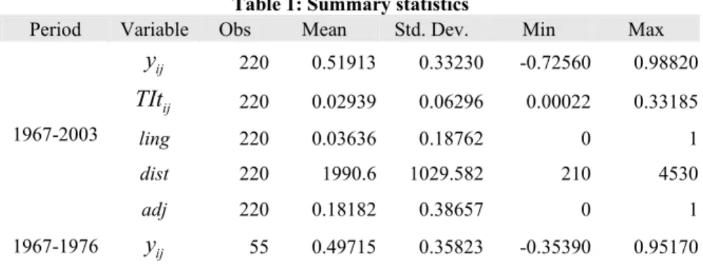
y =corr Q Q , in each of the four sub-periods. Table 1 presents some summary

statistics for the variables considered in the estimation. Figure 1 and 2 present histograms of business cycles correlation and total trade for each sub-period.

Table 1: Summary statistics

Period Variable Obs Mean Std. Dev. Min Max

ij

y 220 0.51913 0.33230 -0.72560 0.98820

ij

TIt 220 0.02939 0.06296 0.00022 0.33185

ling 220 0.03636 0.18762 0 1

dist 220 1990.6 1029.582 210 4530

1967-2003

adj 220 0.18182 0.38657 0 1

ij

TIt 55 0.00806 0.01197 0.00022 0.04309

ij

y 55 0.30947 0.31036 -0.54360 0.92940

1977-1985

ij

TIt 55 0.00791 0.01113 0.00050 0.04113

ij

y 55 0.52111 0.32512 -0.72560 0.95550

1986-1992

ij

TIt 55 0.00934 0.01147 0.00063 0.03775

ij

y 55 0.74879 0.13598 0.46170 0.98820

1993-2003

ij

TIt 55 0.09226 0.10153 0.00760 0.33185

Note: a)y_ij =corr Q Q( _i, _j) where Q_i is the filtered economic activity cycle obtained from the GDP with Baxter-King filter for country i.

b) TIt_ij is the total trade between countries i and j.

c) ling, dist and adj are, respectively, common language, distance and common border.

From Figure 1 we conclude that business cycles correlation is higher on average and much more concentrated around its mean in the last sub-period. From Figure 2 we can also observe an increase in the total trade for the last sub-period.

Figure 1: Histogram of business cycles correlation (y)

0

1

2

3

0

1

2

3

-1 -.5 0 .5 1 -1 -.5 0 .5 1

1967-1976 1977-1985

1986-1992 1993-2003

Hist. of business cycles corr. Hist. of business cycles corr.

Hist. of business cycles corr. Hist. of business cycles corr.

De

ns

it

y

Figure 2: Histogram of total trade (TIt) 0 10 20 30 40 0 10 20 30 40

0 .1 .2 .3 0 .1 .2 .3

1967-1976 1977-1985

1986-1992 1993-2003

Hist. of total trade Hist. of total trade

Hist. of total trade Hist. of total trade

De

ns

it

y

Total Trade:TIt Graphs by period

4.2. Model

Traditional empirical studies relating business cycles correlation and trade intensity employ linear regression models. However business cycles correlation is a limited variable in the interval (-1,1) and the linear regression model is not appropriated since it may yield fitted values outside its range.

In this paper we consider modelling this relationship using the standard beta

distribution. A random variable z is said to follow a beta distribution, with the

parameterization suggested by Ferrari and Cribari-Neto (2004), if its probability density function can be written as,

( ) 1 (1 ( )) 1 ( )

( ; ( ), ) (1 )

( ( ) ) ((1 ( )) )

x x

f z x z z

x x

µ φ µ φ

φ

µ φ

µ φ µ φ

− − −

Γ

= −

Γ Γ − ,

where 0< <z 1, 0<µ( ) 1x < and φ>0. The conditional mean and variance of z are

given respectively by,

E( | )z x =µ( )x ,

and

( )(1 ( ))

Var( | )

1

x x

z x µ µ

φ

− =

+ .

so that ( )µ x is the mean of the response variable an φ can be interpreted as a

precision parameter.

The standard beta distribution is constrained to the unit interval. However it can be

generalized to any interval (a,b). In our case y is a correlation and therefore one would

model z=(y−a) /(b a− )=(y+1) / 2 instead of y, directly. With this transformation

E( | )y x =2E( | ) 1z x −

To model the mean function, E( | )z x =µ( )x , we should consider a specification that

assures it is constrained in the interval (0,1). For this, a useful link is the logit link, exp( ' )

( )

1 exp( ' ) x x x β µ β = + ,

where x is a vector of explanatory variables and β a vector of parameters.

Given a sample of n independent observations, the parameters are estimated by

maximizing the log likelihood function,

1

( , ) ( ; ( ), )

n

i i i

l β φ f y µ x φ

= =

∑

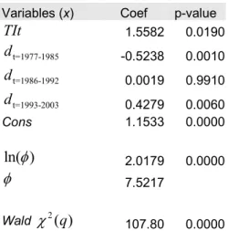
The estimated coefficients are presented in Table 2.

Table 2: Estimated model

Variables (x_{) Coef p-value}

TIt 1.5582 0.0190

t=1977-1985

d _{-0.5238 0.0010}

t=1986-1992

d _{0.0019 0.9910}

t=1993-2003

d _{0.4279 0.0060}

Cons _{1.1533 0.0000}

ln( )φ _{2.0179 0.0000}

φ 7.5217

Wald χ2_{( )q 107.80 0.0000}

Because this is a nonlinear model the estimated coefficient associated with total trade,

TIt, cannot be interpreted as a marginal effect. Since

exp( ' )

E( | ) ( )

1 exp( ' ) x

z x x

x β µ β = = + ,

and x is assumed continuous, the marginal effect of total trade on business cycles

correlation is computed from the derivative,

E( | ) E( | )

2

j j

y x z x

x x

δ δ

δ = δ ,

evaluated at the means of x, x, whose value is given in Table 3, for the whole period.

Table 3: Marginal effet at mean values (1967-2003)

dE(y|x)/dxj

Variable Coef. Std Err

TIt 0.5616 0.2418

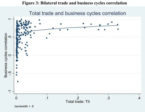
Figure 3: Bilateral trade and business cycles correlation

-1

-.

5

0

.5

1

Bu

si

n

e

ss cycl

e

s

co

rre

la

ti

o

n

0 .1 .2 .3 .4

Total trade: TIt bandwidth = .8

Total trade and business cycles correlation

Figure 4: Estimated business cycles correlation versus total trade

.2

.4

.6

.8

.2

.4

.6

.8

0 .1 .2 .3 0 .1 .2 .3

1967-1976 1977-1985

1986-1992 1993-2003

Estimated y vs. total trade Estimated y vs. total trade

Estimated y vs. total trade Estimated y vs. total trade

mu

=

E(y)

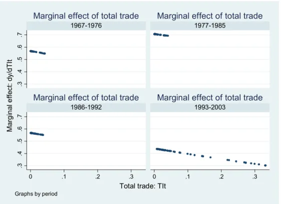
Figure 5: Marginal effect of total trade on business cycles correlation

.3

.4

.5

.6

.7

.3

.4

.5

.6

.7

0 .1 .2 .3 0 .1 .2 .3

1967-1976 1977-1985

1986-1992 1993-2003

Marginal effect of total trade Marginal effect of total trade

Marginal effect of total trade Marginal effect of total trade

M

a

rg

in

al

e

ff

e

c

t:

dy

/d

TI

t

Total trade: TIt Graphs by period

5. Conclusions

In the last four decades, business cycles in eurozone became much more correlated. Europe experienced a unique project of economic and monetary integration with no known precedents in World and the economies gained closer ties. Before the beginning of EMU last stage, in 1999, several other previous steps were taken: free trade arrangements, custom union and, more recently, convergence criteria defined in Maastricht Treaty.

In all this process, trade always was one of the most important variables. An importance justified in the late nineties with the publication of Frankel and Rose “Endogeneity of Optimum Currency Areas Criteria”: This paper showed that trade is positively related with business cycles correlation and, for that reason, a group of countries could become an optimum currency area ex-post, i.e., after the introduction of a common currency. The debate, since then, was about the specific kind of specialization. If it is inter-industry, this relation is negative, but if it is intra-industry, should be positive.

estimates reveal a negative marginal effect with a slope that became more negative in the last decade. This model was applied to eurozone data between 1967 and 2003. Tough this result confirmed the endogeneity hypothesis proposed by Frankel and Rose, it suggests that are trade loosing importance explaining business cycles synchronization, despite this correlation is increasing.

6. References

Artis, M. Is there an European Business Cycle?, CESifo Working Paper, no. 1053, 2003.

Artis, M.; Zhang, W. BInternational Business Cycles and the ERM: Is There a European Business Cycle, International Journal of Finance & Economics, 2 (1), 1997, pp. 1–16.

Babetski, J. EU Enlargement and Endogeneity of some Optimum Currency Area Criteria: Evidence from the CEECs, Czech National Bank, January, 2004.

Bayoumi, T.; Eichengreen, B. BShocking Aspects of European Monetary Integration, In: Torres, F.,Giavazzi, F. Adjustment and Growth in the European Monetary Union, New York: Cambridge University Press, 1993, pp. 193–229.

Baxter, M. And King, R., Measuring Business Cycles: Approximate band-pass filters

for economica time series. The Review of Economics and Statistics, 81(4), pp

575-593, 1999.

Blanchard, O.; Quah, D. The Dynamics Effects of Aggregate Demand and Supply Disturbances, American Economic Review, Q1 4 (79), 1989, pp. 655–673.

Corsetti, G.; Pesenti, P. Self-Validating Optimum Currency Areas, NBER Working Paper, no. 8783, 413 February, 2002.

De Grauwe, P. The Economics of Monetary Union, 5th ed., New York: Oxford University Press, 2003.

De Grauwe, P.; Vanhaverbeke, W. Is Europe an Optimum Currency Area? Evidence from regional data, CEPR Discussion Paper, no. 555, May, 1991.

European Commission. One Market, One Money, New York: Oxford University Press, 1992.

Ferrari and Cribari-Neto, Beta regression for modelling rates and proportions, Journal

of Applied Statistics, vol. 31, nº 7, 2004.

Frankel, J.; Rose, A. The Endogeneity of Optimum Currency Areas Criteria, NBER Working Paper, no 5700, August, 1996.

Frankel, J,; Rose, A. The Endogeneity of Optimum Currency Areas Criteria, The Economic Journal, 421 108 (449), July, 1998, pp. 1009–1025.

Fridmuc, J. The Endogeneity of Optimum Currency Area Criteria, Intra-Industry Trade and EMU Enlargement, Bank of Austria, June, 2001.

Hodrick, R.; Prescott, E. Post-war U.S. Business Cycles: An Empirical Investigation,

Credit and Banking, 29 (1), 1980, pp. 1–16. Hughes Hallett, A.; Piscitelli, L. BEMU in Reality: The Effect of a Common Monetary Policy on Economies with Different Transmission Mechanisms, CEPR Discussion Paper, no. 2068, 1999.

Kenen, P. B. The Theory of Optimum Currency Areas, In: Mundel, R., Swoboda, A.

Monetary Problems of the International Economy, Chicago: Chicago University Press, 1969, pp. 4–60.

Kenen, P. Currency Areas, Policy Domains, and the Institutionalization of Fixed Exchange Rates, Centre for Economic Performance, Discussion Papers, no. 0467, London School of Economics, 2000.

Krugman, P. Lessons of Massachusetts for EMU, In: Torres, F., Giavazzi, F.

Adjustment and Growth in the European Monetary Union, Cambridge: Cambridge University Press, 1993.

Lucas, R. Econometric Policy Evaluation: A Critique, Carneggie-Rochester Conference Series on Public Policy, 1, 1976, pp. 19–46.

Mongelli, F. New Views on the Optimum Currency Area Theory: What is EMU Telling Us?, ECB Working Paper, no. 138, April, 2002.

Mundell, R. BThe Theory of Optimum Currency Areas, American Economic Review, 51 (4), September, 1961, pp. 657–663.

Rose, A. One Money, One Markey? The Effect of Common Currencies on International Trade, Economic Policy, 15 (30), 2000, pp. 7–45.

Rose, A. Meta-Analysis of the Effect of Common Currencies on International Trade,

NBER Working Paper, no. 10373, March, 2004.

Silvestre, J. “Estará a Zona Euro a caminhar para uma Zona Monetária Óptima?,

Master in Economics and European Studies dissertation (supervisor: António Mendonça), Lisbon: Technical University of Lisbon, 2004.