Carlos Pestana Barros & Nicolas Peypoch
A Comparative Analysis of Productivity Change in Italian and Portuguese Airports
WP 006/2007/DE _________________________________________________________
Margarida Chagas Lopes
Time to Complete a Pos-graduation: some evidence of “school effect” upon ISCED 6 trajectories
WP 007/2007/DE/CISEP _________________________________________________________
Departament of Economics
W
ORKINGP
APERSISSN Nº0874-4548
School of Economics and Management
Time to complete a Post-graduation: some evidence on “school effect” upon ISCED 6
trajectories1
Margarida Chagas Lopes2
(http://pascal.iseg.utl.pt/~mclopes )
Technical University of Lisbon (UTL), School of Economics and Management (ISEG)
CISEP – Research Centre on the Portuguese Economy
Abstract
Most Portuguese higher education institutions are increasingly compelled to observe
rather strict arrangements in what concerns time to achieve post-graduation studies. Actually
European equivalence and mobility procedures in the framework of the Bologna process will
not allow for considerable heterogeneity in this light. Nevertheless research carried recently
on four Portuguese higher education institutions’ MSc. and PhD programmes revealed there is
still a large amount of diversity among average time spells required to complete identical
degrees. This outcome suggests that under strict time arrangements Bologna 2nd. and 3rd.
cycles rate of success will widely vary among higher education institutions. Individual
longitudinal data relative to a representative sample of the abovementioned MSc. and PhD.
trajectories allows us to adjust a duration model and thereby investigate some of the main
features behind those so different time spells, that is to say so heterogeneous success patterns.
A quite meaningful “school effect” revealed to be one of the most striking outcomes.
JEL classification: I 23
Keywords: Individual post-graduation trajectories; advanced studies (ISCED 7) organisation;
duration models.
1
Research developed in the framework of Science and Technology Foundation Project Telos II (POCTI/CED/46747/2002).
2
Contents
1. Purpose and General Background
2. Life cycle trajectories and duration models
3. Data
4. Rsults and Discussion
4.1. Adjustment without categorical variable
4.2. Adjustment with categorical variables
Time to complete a Post-graduation: some evidence on “school effect” upon
ISCED 6 trajectories
1. Purpose and General Background
Increasing competitiveness among and for high level skills together with international
policies fostering HRSTE equivalence and mobility both reinforce the role played by
post-graduation programmes assessment (Eggins 2003).
Most research carried on this issue still relies nevertheless upon cross section
methodologies supported by synchronic data most of times. But learning is by itself a
rather complex multidimensional and time dependent process. Likewise analyses on
school success and failure risk neglecting a great deal of the corresponding major
determinants whenever they do not allow for dynamics.
Actually time spells taken by individuals to complete either a Master (MSc.) or a
Doctorate (PhD.) are still quite diverse among and sometimes inside higher education
institutions as it can be confirmed empirically. Therefore it seems quite advisable that
assessment procedures be complemented by specially designed evaluation which should
follow a dynamic methodology supported by longitudinal data on individual
post-graduation trajectories.
Bologna Reform provides a general institutional framework, actually a prerequisite for
further equivalence and mobility. But it will not be powerful enough to foster equal
opportunities among individuals who seek for post-graduation certificates; for those who
come from countries, as Portugal, in which severe limitations have been appointed to
education and training systems chances to become mobile and competitive will inevitably
be fewer. So, it seems to be worthwhile to get a further insight on some of the main
trajectories3, as it will most probably determine further Bologna second and third cycles
rates of success.
Actually, it should be noticed that quite diverse impending restrictions can be at stake
by the time one attends a post-graduation: there can be employment and income
restrictions, family responsibilities, self motivation and resilience, programmes scheduling
and general accessibility, among many other.
OECD Examiners’ Report on higher education in Portugal, for instance, stresses that
“(…) price is a major determinant of student choice (…)” (OECD 2006: 28), an outcome
which doesn’t surprise us given the average level tuition fees can attain against public
social policy narrowness. Most Portuguese post-graduation students have indeed to
depend on a fellowship (or a place in the labour market) as well, according to the
Portuguese Science and Technology Foundation’s (STF) fellowship database. The above
OECD Report states that Graduation students’ motivation depends strongly on the
institutions location and their availability close to the applicant’s residence as well. Will
this same kind of reasons affect also decisions to follow post-graduate studies?
Besides learning obstacles intervening at the time in which a given education level
attendance is taking place many other determinants occur at earlier stages, the role of
which literature and research have been stressing. Among them we must refer to each
individual’s family school level, own previous schooling patterns and the role played by
education institutions successively attended.
Obstacles like the above ones have been emphasized mostly by education sociology
when trying to approach multiple interaction effects exerted by the interplay between
individual and structural factors along life cycle trajectories. By relying upon dynamic
analyses, research of the kind has been enlightening the meaningful role usually played by
one’s previous school record either upon further studying or ulterior employment and
career opportunities. Together with research in economics of education those approaches
outcomes have also been shedding light on the influence exerted by origin (father’s and/or
mother’s) and raised family’s social and educational background upon studies and
3
employment success. Actually they emphasize how these determinants interplay to foster
not only educational access and success (or failure) material requirements but also
background values, beliefs and motivation which shape life cycle trajectories (Plug 2002;
Watson 2003; Devereaux & Salvanes 2004).
Also effects exerted by the education institution upon individual’s opportunities and
success (“school effect”) have been receiving a large concern, mostly in what has to do
with basic and secondary education (Hobcraft 2000; Duru-Bellat 2002; UNICEF 2002).
More recently, in the eve of Bologna agreement, alike research has been developed which
concerns the effects played by higher education institutions (Noyes 2003; Ammermüller
2005).
Research on the Portuguese upper secondary and tertiary patterns has been providing
evidence which confirms the influence exerted by most of the above factors (Chagas
Lopes et all 2004, 2005 a), 2005 b), 2006). Amâncio (2005) and Perista et all (2004),
among other, focus on gender role impact upon graduation and employment opportunities
in Portugal.
So, it seemed to be worthwhile to investigate whether a same kind of reasons could
have any impact upon post-graduation trajectory patterns, as well.
Economic time, e.g. the state of the economy and the labour market by the time when
individuals complete a post-graduation, is also a matter of concern namely when research
is considering post-graduate employment opportunities, which is not the case in this
paper4.
Most of times a compound of the above reasons will be responsible for failure or delay
in studies completion, a great deal of the determinants lying outside the scope of
economics of education. Likewise research approaches on these issues frequently call for
interdisciplinary work, as it is the case with Project Telos II. This should be seen as the
obvious counterpart for trying to build a research methodology robust enough to
disentangle between individuals’ (and their ecosystems) and post-graduation institutions’
4
responsibility for success and failure, an outcome which Bologna Reform should not look
as unworthy, we believe.
Summing up: we intend to assess the joint effect exerted by the abovementioned
determinants, or at least most of them, upon post-graduation trajectories. For that purpose
we take time required to complete a MSc. or a PhD. as an operative proxy for the
dependent variable.
The plan of the paper is as follows: in Section 2 we briefly review literature and
leading issues on life cycle trajectories and duration models. Data description and
questionnaire main contents are addressed in Section 3. In Section 4 we present and
discuss the main outcomes obtained from duration models adjustments, without and with
higher education institution as a categorical variable. Finally, we present the main
conclusions in Section 5.
2. Life cycle trajectories and duration models
Individual longitudinal trajectories have for long deserved increased attention among
research developed in labour economics5.
This growing relevance occurs in the framework of human capital theories criticism
and inscribes into a broader modern approach for which scope the role played by life cycle
theories attracts an increasing concern. The latter main purposes encompass the
identification of the major interactions which take place between education/training and
work/earnings (and family, sometimes) trajectories along individual life cycles6.
Opposite to which happens with those approaches developments in labour market
research, their focus on education and training patterns is deserving a still smaller concern
5
See, for instance, Ben-Porath (1967), Heckman & Macurdy (1980), Willis (1987), Albrecht et all (1991), among other.
6
despite the increasing role played by research on individual decision making relative to
lifelong learning.
Nevertheless, applying life cycle theories to education and training programmes
attendance appears to be quite advisable whenever research concerns the effects exerted
by learning and schooling obstacles upon time needed to complete those programmes.
As far as post-graduate studies are concerned factors such as students’ situation
towards employment and occupational status, learning and career opportunities, family
structure and responsibilities, family’s (father’s and mother’s but also husband’s/wife’s)
human capital, among other, are expected to meaningfully condition both success or
failure outcomes as well as time spells required to complete post-graduation programmes.
Together with the above ones, also individual’s personal characteristics, as age and
gender, own previous schooling landmarks (namely, graduation’s institution, field and
starting and completing dates) and “school effect”, e.g. the influence exerted by
post-graduation institutions upon individual’s learning success, deserve to be investigated. For
that purpose there is a need to assess features such as curricula contents and syllabuses,
course organization and time scheduling, as well as their foreseen adequacy and
pertinence towards further work and career expectations.
When trying to identify such a kind of determinants joint influence upon time spells
required to complete a MSc. or a PhD. applying duration models seems to be particularly
adequate7. Cox proportional hazard models are frequently used to adjust duration models
mostly because they do not impose any specific probability distribution for timeT,
actually a major difficulty most of times. Besides, Cox models allow us to work both with
censored and not censored data, as well.
Likewise, we would let T represent the duration spell needed to complete a
post-graduation programme, being T a random variable with distribution function
( ) ( )
F t =P T ≤t . Therefore, the survivor function would come S t( )=P T( ≥t)and for the
corresponding hazard function we would have h t( )= f t( ) / ( ),S t with f t( ) the density
7
function forT. Adapting duration models conceptualization to the time length required to
complete an advanced studies programme we would say that the hazard function
represents the instantaneous probability of completing the post-graduation at time t, given
the individual was attending it up to that time moment.
For such a duration model, and using the Weibull specification for the baseline
survivor function, we would have (Leão Fernandes, Passos & Chagas Lopes 2004):
( , )
h x t = pt(p-1) exβ
with x representing the characteristic variables, β the corresponding parameters and pstaying for time influence.
Nevertheless, for the specific purpose of this paper we did not consider p, e.g. the
economic time influence. Actually, we are not concerned here with post-graduates’ labour
market insertion conditions once MSc. or PhD. having been completed. Besides, the
relatively close proximity between the two sub-samples completing dates (5 years) did not
allow for meaningful changes in what had to do with most determinants pattern of
influence: cultural and social capital transmission effects are lengthy and evolve slowly as
well as family patterns and also Government transfer and fellowship policies. Even
post-graduation design and organisation arrangements inside institutions were supposed to
remain unchanged along this time interval. Actually, interviews with MSc. and PhD.
coordinators revealed that intervening organisation changes did not meaningfully affect
average duration spells.
Conversely, initial, or previous, conditions, introduced throughout the baseline hazard
( h0 ) concerned us for the reasons we have been describing and therefore we applied
alternatively a continuous time model which proportional hazard rate can be written (see
also Lawless 1982; Kachigan 1986):
( | )
with h0 the baseline hazard function and x the covariates matrix. The corresponding
distribution function being
0
( ) Pr[ ] t ( )
F t = T ≤ =t
∫
f x dxand the survivor function, ( )S t
( ) Pr[
S t = T≥ ] ( )
t
t =
∫
∞ f x dxwith ( )S t continuous, monotonous and decreasing.
Actually, given the methodology applied to the sample design we had not to deal with
censored time intervals, as it will be explained later.
Therefore, we set that time spell required to complete a post- graduation – e.g., the
likelihood that a MSc. would take more than two years to complete – would depend upon:
- initial (baseline) conditions, h0, such as parents’ education level, own
qualifications, field of study, graduation institution and year, situation towards
employment when she/he decided to enrol the post-graduation programme;
- some previously known individual characteristics, like gender, age, place of birth
and residence; other intervening determinants as changing employment and career
status or expectations, changing family structure or size; and post-graduation
institution ( )x .
3. Data
One of the main purposes of Project Telos II consisted in obtaining data on Portuguese
post-graduation patterns in the framework of lifelong learning research studies. The
research methodology design considered the systematic depicting of the sample
Besides this kind of time sensitive data it has also been retrieved a considerable amount of
information on other pertinent fields throughout interviews with post-graduation directors
(UIED 2005), as previously referred.
A survey has been designed and addressed to a representative sample of
post-graduates who had completed a MSc. a PhD., or both, in each one of the four adherent
Portuguese higher education institutions8. This led to address all those who had completed
each one of the above degrees in anyone of the four institutions in the school years
1995-96 and 2000-019:
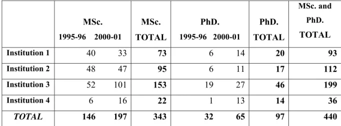
Table 1- Population: Breakdown by Institution, Post-graduation degree and
completing year
MSc.
1995-96 2000-01
MSc.
TOTAL
PhD.
1995-96 2000-01
PhD.
TOTAL
MSc. and
PhD.
TOTAL
Institution 1 40 33 73 6 14 20 93
Institution 2 48 47 95 6 11 17 112
Institution 3 52 101 153 19 27 46 199
Institution 4 6 16 22 1 13 14 36
TOTAL 146 197 343 32 65 97 440
Source: UIED, 2005.
Legend: Institution 1 – New University of Lisbon (FCT)
Institution 2 – Technical University of Lisbon (ISEG)
Institution 3 – University of Aveiro
Institution 4 – University of Lisboa (FPCE)
8
Technical University of Lisbon (School of Economics and Management, ISEG), New University of Lisbon (Faculty of Sciences and Technology), University of Aveiro (Department of Education) and University of Lisboa (Faculty of Psychology and Education).
9
By taking into consideration those two scholar years -1995/96 and 2000/01 – we
would be able to identify and control for the main influence exerted by the economic
cycle upon individuals’ employment opportunities both before and after the
post-graduation attendance, a feature which is not concerning us in this paper.
The sample size was about 33% from that universe (145 individuals) and revealed to
be gender and age representative, 52,4% being the feminization rate and the age
distribution modal class corresponding to the 35-45 years interval. Most respondents (75,2
%) were married/living in a couple with children or other dependents by the time of the
survey; a non negligible number (about 4%) was still living with parents nevertheless.
As to parents’ school level, about 32% among fathers and some 36% among mothers
had not attended school further than the basic education first cycle, actually the most
frequent education level among Portuguese elder population. But some 22% and 29 % (for
fathers’ and mothers’, respectively) were described as performing (or having performed) a
“scientific or intellectual” occupation. Relatively to the husbands’/wives’ school level we
could observe the very well known “endogamic” traits, as expected: most MSc. and PhD.
graduates’ companions have got at least a tertiary level education, about 75,5% among
them performing a “scientific or intellectual” occupation as well. Actually, this is what
since Becker’s approach is usually referred as “assortative mating” (Becker 2005), a
concept which strongly bears within that author’s neo-classical economics focus. A
perspective which has been systematically discussed and set under review by most
sociologists of the family and marriage10.
As an outcome of the survey we obtained data which allowed us to reconstruct 145
post-graduation traectories, being 108 MSc.’s and 37 PhD’s11. For each trajectory it
became possible to establish therefore a time schedule which metric relied upon
post-graduation(s) starting and completing dates (month/year). Likewise we could deal with
closed time intervals for each individual and dated situation avoiding therefore the need to
correct for interval-censored situations. All features we expected to intervene as main
determinants have been dated as well, as we have been describing.
10
For a literature review on this last approach see, for instance, Torres (2001).
11
The main questions addressed by the survey may be described as follows:
- those concerning individuals’ and their close relatives’ personal characteristics,
such as age, gender, place of birth and school level, as well as her/his father’s
/mother’s and husband’s/wife’s school level and occupations;
- questions on each individual’s previous school trajectory, as the field of study
during upper secondary, graduation area, institution and graduation initial and final
year; motivation and reasons to attend post-graduation, as well as the perceived
leading obstacles; higher education institution(s) in which MSc. and/or PhD. had
been completed, as well as the corresponding beginning and completing dates
(month/year);
- questions concerning situation towards employment before, during
post-graduation12 and afterwards, which were classified by occupation, industry, kind of
labour agreement and time to get employment in each search situation;
- family structure: living with parents or raising one’s family, number of children
and/or other relatives before, during and after post-graduation completion;
- respondent’s general assessment on post-graduation main features: syllabuses and
curricula evaluation and adequacy towards occupational requirements, pedagogical
methodologies, contribution to foster skills development, professional attitudes and
personal further learning;
- questions on individual’s sense of fulfilment and satisfaction with the occupational
situation and professional status as a consequence of/after post-graduation
completing.
12
4.Results and Discussion
Our research deals mainly with life cycle transitions, namely in what has to do with
school trajectories and patterns. Likewise, before analysing time influence throughout
duration models we developed an exploratory analysis in order to further investigate on
the transition and dynamic variables main trends.
One of the main questions under research had to do, of course, with studying fields
and possible moving among them from graduation to MSc. and/or PhD. The following
table provides us a meaningful insight on these features:
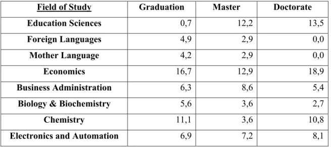
Table 2 - Fields of study: Graduation, Master and Doctorate
Field of Study Graduation Master Doctorate
Education Sciences 0,7 12,2 13,5
Foreign Languages 4,9 2,9 0,0
Mother Language 4,2 2,9 0,0
Economics 16,7 12,9 18,9
Business Administration 6,3 8,6 5,4
Biology & Biochemistry 5,6 3,6 2,7
Chemistry 11,1 3,6 10,8
Electronics and Automation 6,9 7,2 8,1
Source: UIED, 2005
According to the table it seems three leading patterns can be depicted: i) some fields,
like Education Sciences, appear mostly as destination fields, as almost no individual
among the sample graduate in that area; ii) some other, as Foreign and Mother Languages,
seem to appear mostly as career starting domains, the corresponding MSc. and PhD. fields
lying in different research areas, most probably the Education Sciences one; iii) for the
PhD., an outcome which appears mostly striking in Economics, Chemistry and
Electronics.
The above results are expected to affect individual mobility among higher education
institutions when trying to advance towards higher degrees. Actually only 10 among the
145 individuals kept in the same institution from Graduation to PhD, 5 among them in one
of the institutions providing Graduation, MSc. and PhD in Economics.
Another feature requiring a further insight concerns the need to breakdown between
individuals following an academic career and other professionals. Actually, either reasons
and motivations, obstacles and constraints, further occupational outcomes and degree of
fulfilment… will strongly depend upon that decomposition. Analysing the database we
can observe that about one half of the sample individuals (48, 9%) were following an
academic career: 45 among MSc’s and 26 among PhD’s.
To further clarify this latter issue, we applied Contingency Analysis to “time required
to complete a MSc.” and “pursuing an academic career” and obtained for the
χ
2significance level a value equal to 0,081, quite close to the 0,05 tolerance level.
Proceeding identically for PhD., we obtained no conclusive outcome giving the small
number of individuals in this situation. The above results advised us to deal with this
feature with most precaution when applying duration models.
Both exploratory analyses and parallel research on this same database have showed
that gender effects exert a very strong influence upon individuals’ time to complete
post-graduate studies (Chagas Lopes 2006). Therefore every adjustment we made has been
stratified by sex, although we will not discuss here the corresponding outcomes.
As to location, a feature we must remember OECD Examiners’ Report includes
among the main obstacles to further studying, we also investigated on its effect.
Contingency Analyses did not confirm association between higher education institutions
(Graduation, MSc. or PhD) and either origin or present residence location.
residence location (
χ
2 significance level equal to 0,039), a feature which will not concernus as we are dealing with post-graduation trajectories.
As previously referred we are particularly concerned with the influence exerted by
higher education institutions, among other variables, upon time spells individuals need to
complete graduation. Despite Contingency Analyses did not unequivocally allow for those
variables association, we assume that a great deal of other variables intervening
throughout higher education institution may affect those time spells. Therefore, we tried to
assess those variables joint influence upon post-graduation duration.
In face of the obvious differences between MSc. and PhD. grades in as much as
attendance reasons, potential obstacles and success/failure rates are concerned we decided
to analyse separately the corresponding situations. Likewise we considered at a time either
the 108 MSc. or the 37 PhD. trajectories.
As previously referred (Section 2) we applied Cox proportional hazard models to
adjust for our concerning variables (covariates) joint influence upon time length required
to complete a MSc. or a PhD. once started. For the dependent variable, e.g. time needed to
complete either degree (or conversely, the probability that a MSc./PhD. would take, for
instance, longer than two years to complete) we computed it for each observation by
subtracting starting from completing dates once normalised.
Covariates were selected from the database according to literature outcomes, our
research hypothesis developed in Sections 1. and 2. and the above exploratory results. On
account of the outcomes we previously obtained for gender association with other
variables we decided to set sex as a stratification categorical variable, thereby allowing for
separate baseline hazard functions for women and for men.
Also for each grade (MSc. and PhD.) we alternatively computed adjustments
without/with higher education institution as a categorical variable. Likewise, in this latter
situation we could disaggregate among different higher education institutions specific
influence and consider, or not, it to be influent according to the value for the overall Wald
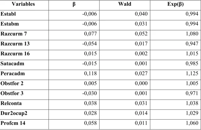
4.1.- Adjustment without categorical variable
The adjustment for MSc. trajectories with no categorical variable provided an
acceptable outcome according to the overall tests and scores13(See Appendix 1).
Adjustment outcomes displayed by SPSS (version 15.0) provide not only values for the
unstandardized regression coefficients β, which cannot be used for prediction, but also
some corresponding tests, as the Wald test significance: whenever the latter will be equal
or lower than 0,05 the corresponding variable will be considered relevant. Therefore, the
following variables and influence have been accepted: Graduation and Master institutions
(establ; estabm); several reasons to have completed MSc. (being able to perform the
desired occupation – razcurm 7; employer’s demanding – razcurm 13; wish to studying
further – razcurm 16 and wish to develop own scientific culture – procfm 14); satisfaction
with academic work and career (satacadm and peracadm, respectively); lack of support by
employer and family (obstfor 2 and obstfor 3, respectively); present occupation status in
terms of kind of labour agreement and tenure (relconta; dur2ocup2).
Additionally, in a model like the current one positive values for the coefficients are
equivalent to higher values for the hazard function or, conversely, shorter durations (Box
– Steffensmeier & Zorn 1998). Thus, negative values for covariates coefficients – whether
acceptable – will mean the corresponding variables will affect positively time duration,
e.g., will imply longer time spells. This is the case with establ and estabm, razcurm13,
satacadm e obstfor3, which means that longer durations are mostly induced by previous
and present scholar institutions, employer’s behaviour, own degree of satisfaction towards
academic career and lack of support by family.
13
Table 3 - Variables in the Equation (main scores ant tests)
Variables β Wald Exp(β)
Establ -0,006 0,040 0,994
Estabm -0,006 0,031 0,994
Razcurm 7 0,077 0,052 1,080
Razcurm 13 -0,054 0,017 0,947
Razcurm 16 0,015 0,002 1,015
Satacadm -0,015 0,001 0,985
Peracadm 0,118 0,027 1,125
Obstfor 2 0,005 0,000 1,005
Obstfor 3 -0,030 0,001 0,971
Relconta 0,038 0,031 1,038
Dur2ocup2 0,028 0,014 1,029
Profcm 14 0,058 0,011 1,060
Legend: Establ – Graduation institution; Estabm – Master institution; Razcurm 7 – Preparing to
perform the desired occupation; Razcurm 13 – Employer’s demanding; Satacadm – Satisfaction with
academic work; Peracadm – Satisfaction with academic career; Obstfor 2 – Lack of support by employer;
Obstfor 3 – Lack of support by family; Relconta – Nature of labour agreement present occupation;
Dur2ocup2 – Present occupation tenure; Profcm 14 – Wish to develop own scientific culture.
From the above table we can also observe values for Exp(β), or the Odds ratios, from
which values we can infer the predicted change in the hazard function induced by each
variable: the higher the Odds (above 1,0) the larger the expected influence. Therefore,
degree of satisfaction with academic career (peracadm), becoming able to perform the
wished occupation (razcurm 7), wish to develop scientific culture (profcm 14) and, in a
smaller way, present occupation (by the time of the enquiry) statutory conditions (relconta
and dur2ocup2) all exert an amplifying effect.
Features concerning academic occupations and career appear therefore to be the most
and research requirements, some of the corresponding occupations and career
administrative arrangements, and sense of fulfilment with this kind of occupation, all of
them seem to be at stake now. It also deserves to be mentioned that either Graduation and
MSc. institutions play a highly meaningful role in as far as time each individual has
required to complete a MSc. is concerned. Notwithstanding some matter of concern arises
from the apparent contradictory role played by employers: either it seems they set MSc.
achievement as a goal or a requirement to be met or they appear among the main obstacles
to its completing, together with family. Were there be no further reasons, this single
outcome led us to conclude on the probable heterogeneity of the surveyed population.
Therefore it appeared to be most advisable to advance throughout a more disaggregated
analysis.
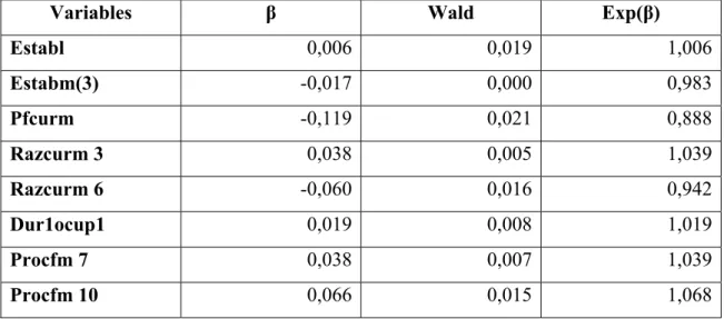
4.2.- Adjustment with categorical variable
When we set a given variable as a categorical one the corresponding values will
perform the role of dummies and compare with the reference (omitted) one. In the present
situation each MSc. /PhD. institution has been codified as many times as the number of
questioned programmes leading to a different grade, e.g. seven. Results for MSc. Cox
regression adjustment setting the institution as categorical (indicator) variable are shown
in Appendix 2. It is worth to be mentioned that this second outcome provided better
results for the overall statistical tests than the previous one (overall Qui-square
significance level now equal to 0,002, against a former value equal to 0,007).
Nevertheless the Wald test for the joint MSc. institutions presents now a value which
does not unequivocally state for the influence exerted by each one of them, except for
“estabm(3)”. Considering covariates significance level (S, see Appendix 2) as an
additional test, both “estabm(3)”, “estabm(1)” and to a lesser extent “estabm(2)” appear to
exert a meaningful despite symmetrical influence upon time spells required to complete a
Master14. According to β signs, it seems that shorter durations appear to be associated with
“estabm(2)” and “estabm(6)”, these same two institutions seeming to exert larger impacts
as well in view of the values associated with the corresponding Exp(β).
14
As to the other covariates effects we must emphasize the following ones: Graduation
institution (establ), kind of occupation after MSc. completing (pfcurm), some of the
reasons to have attended a Master (being able “to change” or to “perform better” one’s
employment – razcurm 3 and razcurm 6, respectively, together with aiming to improve
“participation in work organisation” - procfm 10 and, more pragmatically, just the sake
for obtaining a MSc. certificate – procfm 7) and first occupation tenure (dur1ocup1).
Now, shorter durations seem to be associated with previous Graduation institution
(establ), wishing to change from employment (previous or coincident to post-graduation
attendance) and first employment tenure (razcurm 3 and dur1ocup1, respectively), wish to
participate in work organisation (procfm 10) or simply seeking for a MSc. certificate
(procfm 7). Only Master institution, kind of occupation after MSc. completing and wish to
perform better her/his own job, appear now as implying longer time spells duration. At the
same time, only three variables seem to exert now a meaningful amplifier effect,
according to values exhibited by Exp(β): preparing for participating in work organisation
(procfm 10), seeking for a MSc. certificate (procfm 7) and preparing to change
employment (razcurm 3).
Table 4 - Variables in the Equation (main scores ant tests)
(estabm as categorical)
Variables β Wald Exp(β)
Establ 0,006 0,019 1,006
Estabm(3) -0,017 0,000 0,983
Pfcurm -0,119 0,021 0,888
Razcurm 3 0,038 0,005 1,039
Razcurm 6 -0,060 0,016 0,942
Dur1ocup1 0,019 0,008 1,019
Procfm 7 0,038 0,007 1,039
Procfm 10 0,066 0,015 1,068
Legend: Establ – Graduation institution; Estabm – Master institution; Pfcurm – Occupation after
Master completing Razcurm 3 – Preparing to change employment; Razcurm 6 –Preparing to perform
better own employment; Du1ocup1 – First occupation tenure; Profcm 7 – Seeking for a Master certificate; .
Profcm 10 – Preparing for participation in work organisation.
We should notice as well that two evaluation criteria variables almost reached the
significance level tolerance threshold (See Appendix 2): “quality and adequacy of the
programme equipment and pedagogical resources” (avalfm 9) and, in a lesser extent,
“curricula adequacy towards own learning purposes” (avalfm 1), two outcomes which we
will keep for further research.
Now other reasons and motivations different from strict academic purposes could
appear. Actually, we can now wonder how far investing in a MSc. could have been
designed as a professional mobility strategy, a way to improve one’s ability to intervene in
work conditions and perhaps also a device to fight against labour precariousness
(considering “dur1ocup1”). Clearly, own previous scholar trajectory could appear again as
*
* *
Applying the same methodology to investigate time required to complete a PhD.
proved to be unsuccessful and we obtained no convergent adjustment. This result did not
surprise us given the few number of doctorate trajectories present in the work sample.
Trying to improve the possible characterization of this latter kind of trajectories we
developed some complimentary statistical analyses (using Contingency and Discriminant
techniques) and thereby were able to state that two single variables appeared to exert a
meaningful influence: “wish to develop own studies and knowledge” and “mother’s
school level”. Will this apparent association be in line with most doctorate’s graduation
fields, e.g. scientific and cultural occupations and teachers’ training? That’s just a
hypothesising question, reliable conclusions on this issue absolutely requiring a more
robust database.
5. Conclusion
Despite data limitations we think our main purposes have been fulfilled which may
serve as a starting point for further more in depth analyses.
First of all we shed light into adequacy of longitudinal data for research on time
dependent processes as it is the case with school and learning degrees. Actually we
obtained rather systematic outcomes in which concerns the role played by most
determinants and leading issues affecting duration of time spells needed to achieve
post-graduation studies.
A first meaningful result concerns mobility among studying fields and, as a
consequence, among higher education institutions, mostly between Graduation and MSc’s
but also towards PhD’s institutions. Contingency analysis displayed a strong association
between Graduation institution and place of residence, an outcome which goes in line with
accessibility restrictions appeared to intervene as a major obstacle for post-graduate
studies, both for Lisbon institutions’ and also Aveiro University’s post-graduates.
Duration model adjustment without categorical variable displayed outcomes which we
considered quite biased on account of academic trajectories influence, which nevertheless
amount to no more than roughly 50% of the whole sample: both duration trends and
amplifying effects proved to be quite contingent on academic career variables, as well as
on work and family ones.
Readjusting the model by setting MSc. establishment as a categorical variable it
became therefore possible to disaggregate among two kinds of MSc. institutions and
programmes: those mostly featured to provide academic professionals, and the more
transversal ones addressed to broader occupational fields. We could obtain quite diverse
outcomes relatively to MSc. institutions and programmes, both in what concerns duration
trends and magnitude of effects. Now, also occupational and professional reasons – other
than academic ones – proved to be quite meaningful in shortening duration spells: among
them we emphasize those associated with previous occupations’ statuses, mobility
strategies and even a “credential effect”, the latter introduced by a non negligible number
of respondents who referred just the sake for obtaining a MSc. certificate among their
leading motivations.
Labour market reasons seem to play, indeed, a major role. Either under the form of
academic career and corresponding requirements or whenever MSc. intentionally plays
the role of job search, horizontal or upward mobility strategies in which concerns other
occupation’s trajectories. In either situation also the willingness to improve one’s
knowledge and further learning could be derived as a meaningful outcome, this result
requiring a more robust data support in further research.
Family effects are quite obvious as well: they became particularly evident throughout
most respondents’ answers signalling them among obstacles to complete MSc. within a
shorter time spell. Perhaps also mother’s school level - the only family’s “human capital”
among the outcomes - will be affecting most PhD. patterns and determinants but results
were not conclusive enough on this feature neither were they relatively to the other PhD.
In either model Graduation establishment revealed to exert a relevant influence upon
time duration. Heterogeneity among post-graduation institutions relatively to features
under review revealed to be quite obvious, as well. Therefore we are now able to
disentangle among the ones in where a MSc. takes less time and the other which perform
worse under this point of view. And we also obtained meaningful signalling on which
institutions (from the respondents’ point of view) offer the most interesting curricula and
are considered better equipped among the ones which the Project researched.
Actually, the role played by education institutions, both Graduation and Master ones,
appeared to be most relevant. This outcome allows us to state that an important “school
effect” will go on affecting school trajectories into a further path – post-graduate studies –
than the ones with which research is usually concerned, as we had previously set as a
Bibliography
• Albrecht, J. et al (1991), “Career interruptions and subsequent earnings: a
reexamination using Swedish data”, Journal of Human Resources 34, 249-311;
• Amâncio, L. (2005), “Reflections on science as a gendered endeavour: changes and
continuities”, Social Science Information, vol. 44, nº1, 65-83;
• Ambrósio, T. et al (2006), Projecto Telos II – Aprendizagem ao Longo da Vida:
Efeitos em Diplomados de Ensino Superior, POCTI/CED/46747/2002, Monte de
Caparica, UIED-FCT/UNL;
• Ammermüller, A. (2005), “Educational Opportunities and the Role of Institutions”,
Research Memoranda 004, Maastricht, ROA;
• Becker, G. (2005), A treatise on the Family (enlarged edition), Harvard University Press, Harvard;
• Ben-Porath, Y. (1967), “The production of human capital and the life cycle of
earnings”, Journal of Political Economy 75; 353-367;
• Black, S. et al (2003), “Why the apple doesn’t fall far: understanding intergenerational transmission of human capital”, American Economic Review 95(1), 437-449;
• Bollens, J. & Ives Nicaise (1994), “The medium-term impact of vocational training on
employment and unemployment duration “, Warsaw EALE Conference, 22-25
September;
• Box-Steffensmeier, J. & Christopher Zorn (1998), “Duration Models and Proportional Hazards in Political Science”, Department.of Political Science, Ohio State University,
Columbus;
• Chagas Lopes, M. et al (2004), « School failure and intergenerational «human capital»
transmission in Portugal”, Education-online, ECER/EERA Annual Conference,
University of Crete, 22-25 September;
• Chagas Lopes, M. et al (2005 a)), “Trajectórias Escolares, Inserção Profissional e
Desigualdades Laborais: uma análise de género”, Projecto
FCT/PIHM/ECO49741/2003, Lisboa, CISEP/ISEG-UTL;
• Chagas Lopes, M. et al (2005 b)), “Does school improve equity? Some key findings
from Portuguese data”, Education-online, ECER/EERA Annual Conference, Dublin,
• Chagas Lopes, M. (2006), “Portuguese women in Science and Technology (S&T):
some gender features behind MSc. and PhD. achievement”, Education-online,
ECER/EERA Annual Conference, Geneve, 7-9 September;
• Duru-Bellat, M. (2002), “Les inégalités sociales à l’école et l’IREDU : vingt-cinc ans de recherches’’, IREDU, Université de Bourgogne ;
• Eggins, H. (2003), ‘’Globalization and reform : necessary conjunctions in higher
education”, Globalization and Reform in Higher Education, UK, SRHE and Open
University Press;
• Garson, D. (2005), Statnotes: An Introduction to Multivariate Analysis, Statistic
Solutions (http://www.statisticssolutions.com );
• Heckman, J. & Thomas Macurdy (1980), “A life cycle model of female labour
supply”, The Review of Economic Studies, vol 47, nº1, 47-74;
• Hobcraft, J. (2000), “The roles of schooling and educational qualifications in the
emergence of adult social exclusion”, London, LSE Casepaper nº 43;
• Kachigan, S. (1986), Statistical Analysis – An Interdisciplinary Introduction to
Univariate & Multivariate Methods, New York, Radius Press;
• Lawless, J. (1982), Statistical Models and Methods for Lifetime Data, New York,
Wiley & Sons;
• Leão Fernandes, G. et al (2004), ‘’Skill development patterns and their impact on
reemployability: evidence for Portugal”, TLM.NET Conference Managing Social
Risks through Transitional Labour Markets, SISWO, University of Amsterdam;
• Noyes, A. (2003), “School transfer and social relocation”, International Studies in Sociology of Education, XIII (3);
• OECD (2006), Reviews of National Policies for Education – Tertiary Education in
Portugal: Examiners’ Report, Paris, OECD – Directorate for Education /Education
Committee (06/12/2006);
• Perista, H. & Alexandra Silva (2004), Science Careers in Portugal,
MOBISC-EURODOC, Bruxelas, Comissão Europeia;
• Plug, E. (2002), “How do parents raise the educational attainment of future
generations?”, Bonn, IZA DP nº65;
• Torres, A. (2001), Sociologia do Casamento. A Família e a Questão Feminina, Oeiras,
Celta Editora;
• Watson, T. (2003), Sociology, Work and Industry, UK, Routledge;
• Weiss, Y. (1986), “The determinants of life cycle earnings: a survey”, In Orley
Ashenfelter & Richard Layard (publs.) Handbook of Labour Economics, Amsterdam,
North Holland;
• Willis, R. (1986), “Wage Determinants: a Survey and Reinterpretation of Human
Capital Earnings Function”, In Orley Ashenfelter & Richard Layard (publs.)
APPENDIX 1
Block 1: Method = Enter
Cox Regression
[DataSet1] D:\BASE TELOS.sav
Case Processing Summary
108 100,0% 0 ,0% 108 100,0% 0 ,0% 0 ,0% 0 ,0% 0 ,0% 108 100,0% Eventa Censored Total Cases available in analysis
Cases with missing values
Cases with negative time Censored cases before the earliest event in a stratum
Total Cases dropped
Total
N Percent
Dependent Variable: Data Inic/Data Fim Mest Tratada a.
Stratum Statusa
masculino 47 0 ,0%
feminino 61 0 ,0%
108 0 ,0%
Stratum 1 2 Total
Strata label Event Censored
Censored Percent
The strata variable is : Género a.
Block 0: Beginning Block
Omnibus Tests of Model Coefficients
719,255 -2 Log Likelihood
Block 1: Method = Enter
Omnibus Tests of Model Coefficientsa,b
614,731 123,544 88 ,007 104,523 88 ,110
-2 Log
Likelihood Chi-square df Sig. Overall (score)
Chi-square df Sig. Change From Previous Step
Page 1
Omnibus Tests of Model Coefficientsa,b
104,523 88 ,110 Chi-square df Sig.
Change From Previous Block
Beginning Block Number 0, initial Log Likelihood function: -2 Log likelihood: 719,255 a.
Beginning Block Number 1. Method = Enter b.
Variables in the Equationb
,281 ,377 ,556 1 ,456 1,325 ,633 2,774
-,002 ,001 8,862 1 ,003 ,998 ,997 ,999
-,003 ,008 ,136 1 ,712 ,997 ,981 1,013
,816 ,237 11,804 1 ,001 2,261 1,420 3,600
-,574 ,247 5,370 1 ,020 ,564 ,347 ,915
,239 ,107 4,973 1 ,026 1,270 1,029 1,567
,002 ,001 1,676 1 ,196 1,002 ,999 1,004
-,001 ,001 2,793 1 ,095 ,999 ,997 1,000
,001 ,003 ,205 1 ,650 1,001 ,996 1,007
-,001 ,003 ,312 1 ,576 ,999 ,993 1,004
-,004 ,003 1,471 1 ,225 ,996 ,990 1,002
-,006 ,031 ,040 1 ,842 ,994 ,936 1,055
-,006 ,032 ,031 1 ,859 ,994 ,934 1,058
-1,008 ,335 9,086 1 ,003 ,365 ,189 ,703
1,094 1,037 1,113 1 ,291 2,987 ,391 22,810
,346 ,460 ,564 1 ,453 1,413 ,573 3,484
-,278 ,644 ,186 1 ,667 ,758 ,214 2,678
1,160 ,515 5,075 1 ,024 3,191 1,163 8,756
,002 ,002 1,354 1 ,245 1,002 ,999 1,006
-,178 ,425 ,175 1 ,675 ,837 ,364 1,925
,748 ,332 5,064 1 ,024 2,112 1,101 4,050
-,480 ,483 ,990 1 ,320 ,619 ,240 1,594
-,263 ,554 ,225 1 ,635 ,769 ,259 2,279
,233 ,369 ,397 1 ,529 1,262 ,612 2,602
,157 ,469 ,112 1 ,738 1,170 ,467 2,932
,077 ,337 ,052 1 ,819 1,080 ,557 2,093
,142 ,338 ,176 1 ,675 1,152 ,594 2,236
,251 ,245 1,056 1 ,304 1,286 ,796 2,077
,948 ,545 3,029 1 ,082 2,582 ,887 7,512
-,626 ,261 5,753 1 ,016 ,535 ,321 ,892
-1,036 ,557 3,461 1 ,063 ,355 ,119 1,057
-,054 ,419 ,017 1 ,897 ,947 ,417 2,153
-,214 ,467 ,210 1 ,647 ,807 ,323 2,016
,318 ,350 ,826 1 ,364 1,375 ,692 2,733
,015 ,317 ,002 1 ,963 1,015 ,545 1,888
-,976 ,624 2,446 1 ,118 ,377 ,111 1,280
-,015 ,406 ,001 1 ,971 ,985 ,445 2,184
,118 ,718 ,027 1 ,869 1,125 ,275 4,601
-,475 ,538 ,781 1 ,377 ,622 ,217 1,784
,005 1,430 ,000 1 ,997 1,005 ,061 16,589
-,030 1,262 ,001 1 ,981 ,971 ,082 11,505
datanac1 concres sitfamil nivescp nivescm nivesc profissp profissm profissc areafor1 areafor2 establ estabm diflic1 profcurm exigcarm pfcurm outcursm arfcurm razcurm1 razcurm2 razcurm3 razcurm4 razcurm5 razcurm6 razcurm7 razcurm8 razcurm9 razcur10 razcur11 razcur12 razcur13 razcur14 razcur15 razcur16 razcur17 satacadm peracad obstfor1 obstfor2 obstfor3
B SE Wald df Sig. Exp(B) Lower Upper
95,0% CI for Exp(B)
Variables in the Equationb
-,227 ,619 ,134 1 ,714 ,797 ,237 2,683
. 0a .
. 0a .
-4,564 2,535 3,242 1 ,072 ,010 ,000 1,498
-4,508 2,018 4,992 1 ,025 ,011 ,000 ,575
-,895 ,743 1,453 1 ,228 ,409 ,095 1,752
,513 ,906 ,320 1 ,572 1,670 ,283 9,863
1,922 2,102 ,836 1 ,361 6,836 ,111 420,898
2,388 1,488 2,575 1 ,109 10,894 ,589 201,357
-1,612 ,840 3,684 1 ,055 ,200 ,039 1,035
-,550 ,386 2,031 1 ,154 ,577 ,271 1,229
-,035 ,091 ,149 1 ,700 ,965 ,807 1,154
-,004 ,003 1,341 1 ,247 ,996 ,990 1,002
,004 ,007 ,260 1 ,610 1,004 ,990 1,017
,386 ,368 1,101 1 ,294 1,471 ,715 3,027
-,143 ,454 ,100 1 ,752 ,866 ,356 2,111
-,133 ,203 ,431 1 ,512 ,875 ,588 1,303
,038 ,213 ,031 1 ,860 1,038 ,684 1,577
,199 ,166 1,433 1 ,231 1,220 ,881 1,691
,028 ,240 ,014 1 ,906 1,029 ,643 1,647
-,209 ,453 ,213 1 ,644 ,811 ,334 1,972
,158 ,115 1,894 1 ,169 1,171 ,935 1,466
-,981 ,519 3,573 1 ,059 ,375 ,136 1,037
-,438 ,731 ,359 1 ,549 ,645 ,154 2,702
1,088 ,641 2,878 1 ,090 2,968 ,845 10,429
-1,288 ,485 7,052 1 ,008 ,276 ,107 ,714
1,277 ,624 4,190 1 ,041 3,584 1,056 12,170
,584 ,437 1,788 1 ,181 1,793 ,762 4,223
-2,279 ,536 18,062 1 ,000 ,102 ,036 ,293
-,344 ,516 ,444 1 ,505 ,709 ,258 1,949
1,272 ,642 3,926 1 ,048 3,567 1,014 12,548
,315 ,415 ,578 1 ,447 1,371 ,608 3,089
,561 ,438 1,636 1 ,201 1,752 ,742 4,136
,653 ,665 ,964 1 ,326 1,922 ,522 7,079
1,098 ,540 4,134 1 ,042 2,998 1,040 8,640
-1,373 ,460 8,918 1 ,003 ,253 ,103 ,624
1,851 ,534 11,990 1 ,001 6,364 2,233 18,143
-1,920 ,493 15,174 1 ,000 ,147 ,056 ,385
-,426 ,390 1,194 1 ,275 ,653 ,305 1,402
1,060 ,408 6,752 1 ,009 2,887 1,298 6,425
,655 ,504 1,688 1 ,194 1,926 ,717 5,177
,260 ,475 ,300 1 ,584 1,298 ,511 3,294
-1,014 ,533 3,614 1 ,057 ,363 ,128 1,032
-,722 ,552 1,712 1 ,191 ,486 ,165 1,433
-,113 ,326 ,121 1 ,728 ,893 ,471 1,691
,058 ,565 ,011 1 ,918 1,060 ,350 3,207
,895 ,744 1,446 1 ,229 2,447 ,569 10,521
,933 ,550 2,872 1 ,090 2,542 ,864 7,476
6,900 3,052 5,110 1 ,024 992,188 2,503 393358,12 obstfor4 obstfor5 obstfor6 obstfor7 obstfor8 obstfor9 obstfo10 obstfo11 obstfo12 obstfo13 finobstf propcurs profocp prfocupa sitprof sitprofa relcont relconta dur1ocp1 dur2ocp2 ocprofac nemp trajprof avalfm1 avalfm2 avalm3 avalfm4 avalfm5 avalfm6 avalfm7 avalfm8 avalfm9 procfm1 procfm2 procfm3 procfm4 procfm5 procfm6 procfm7 procfm8 procfm9 procfm10 procfm11 procfm12 procfm13 procfm14 procfm15 procfm16 procfm17
B SE Wald df Sig. Exp(B) Lower Upper
95,0% CI for Exp(B)
Degree of freedom reduced because of constant or linearly dependent covariates a.
Constant or Linearly Dependent Covariates S = Stratum effect. obstfor5 = 0 + S ; obstfor6 = 0 + S ; b.
Page 3
Data Inic/Data Fim Mest Tratada
10 8 6 4 2 0 Cum Survival 1,0 0,8 0,6 0,4 0,2 0,0 feminino masculino Género Survival Function at mean of covariates
Data Inic/Data Fim Mest Tratada
8 6
4 2
0
Cum Hazard
80
60
40
20
0
feminino masculino Género Hazard Function at mean of covariates
APPENDIX 2
Cox Regression
Case Processing Summary
108 100,0% 0 ,0% 108 100,0% 0 ,0% 0 ,0% 0 ,0% 0 ,0% 108 100,0% Eventa Censored Total Cases available in analysis
Cases with missing values
Cases with negative time Censored cases before the earliest event in a stratum
Total Cases dropped
Total
N Percent
Dependent Variable: Data Inic/Data Fim Mest Tratada a.
Stratum Statusa
masculino 47 0 ,0%
feminino 61 0 ,0%
108 0 ,0%
Stratum 1 2 Total
Strata label Event Censored
Censored Percent
The strata variable is : Género a.
Categorical Variable Codingsb
1 1 0 0 0 0 0
43 0 1 0 0 0 0
10 0 0 1 0 0 0
1 0 0 0 1 0 0
1 0 0 0 0 1 0
27 0 0 0 0 0 1
25 0 0 0 0 0 0
0 1 8 12 15 26 36 estabma
Frequency (1) (2) (3) (4) (5) (6)
Indicator Parameter Coding a.
Category variable: estabm (Estabelecimento mestrado) b.
Block 0: Beginning Block
Omnibus Tests of Model Coefficients
719,255 -2 Log Likelihood
Page 1
Block 1: Method = Enter
Omnibus Tests of Model Coefficientsa,b
605,681 138,591 93 ,002 113,573 93 ,072
-2 Log
Likelihood Chi-square df Sig. Overall (score)
Chi-square df Sig. Change From Previous Step
Omnibus Tests of Model Coefficientsa,b
113,573 93 ,072 Chi-square df Sig.
Change From Previous Block
Beginning Block Number 0, initial Log Likelihood function: -2 Log likelihood: 719,255 a.
Beginning Block Number 1. Method = Enter b.
Variables in the Equationb
-,251 ,442 ,324 1 ,569 ,778 ,327 1,848
-,002 ,001 15,588 1 ,000 ,998 ,996 ,999
-,009 ,009 ,824 1 ,364 ,991 ,973 1,010
1,029 ,276 13,906 1 ,000 2,797 1,629 4,804
-,644 ,285 5,118 1 ,024 ,525 ,300 ,918
,411 ,127 10,493 1 ,001 1,508 1,176 1,933
,004 ,002 6,435 1 ,011 1,004 1,001 1,007
-,002 ,001 2,139 1 ,144 ,998 ,996 1,001
-,006 ,004 2,070 1 ,150 ,994 ,986 1,002
-,002 ,003 ,434 1 ,510 ,998 ,991 1,004
-,004 ,004 1,093 1 ,296 ,996 ,987 1,004
,006 ,045 ,019 1 ,890 1,006 ,921 1,099
9,045 6 ,171
-1,115 2,387 ,218 1 ,640 ,328 ,003 35,267
2,030 1,504 1,822 1 ,177 7,618 ,399 145,277
-,017 1,873 ,000 1 ,993 ,983 ,025 38,652
-6,364 3,726 2,918 1 ,088 ,002 ,000 2,554
10,290 4,785 4,625 1 ,032 29441,146 2,490 3,5E+008
2,602 ,971 7,180 1 ,007 13,495 2,011 90,541
-1,477 ,437 11,414 1 ,001 ,228 ,097 ,538
1,216 1,173 1,074 1 ,300 3,373 ,338 33,614
,161 ,529 ,093 1 ,761 1,175 ,417 3,311
-,119 ,821 ,021 1 ,885 ,888 ,178 4,435
1,539 ,602 6,542 1 ,011 4,660 1,433 15,157
,006 ,003 5,397 1 ,020 1,006 1,001 1,011
-,676 ,496 1,860 1 ,173 ,509 ,192 1,344
1,288 ,505 6,509 1 ,011 3,624 1,348 9,744
,038 ,523 ,005 1 ,941 1,039 ,373 2,899
-,285 ,522 ,299 1 ,585 ,752 ,270 2,091
,402 ,399 1,015 1 ,314 1,495 ,684 3,268
-,060 ,482 ,016 1 ,901 ,942 ,366 2,424
datanac1 concres sitfamil nivescp nivescm nivesc profissp profissm profissc areafor1 areafor2 establ estabm estabm(1) estabm(2) estabm(3) estabm(4) estabm(5) estabm(6) diflic1 profcurm exigcarm pfcurm outcursm arfcurm razcurm1 razcurm2 razcurm3 razcurm4 razcurm5 razcurm6
B SE Wald df Sig. Exp(B) Lower Upper
95,0% CI for Exp(B)
Variables in the Equationb
-,476 ,412 1,339 1 ,247 ,621 ,277 1,391
-,485 ,431 1,265 1 ,261 ,616 ,265 1,433
,497 ,276 3,235 1 ,072 1,643 ,956 2,823
2,039 ,709 8,269 1 ,004 7,685 1,914 30,854
-,498 ,312 2,549 1 ,110 ,608 ,330 1,120
-1,626 ,712 5,214 1 ,022 ,197 ,049 ,794
,423 ,610 ,482 1 ,488 1,527 ,462 5,046
-1,441 ,709 4,127 1 ,042 ,237 ,059 ,951
,897 ,429 4,380 1 ,036 2,453 1,059 5,684
-,345 ,350 ,969 1 ,325 ,708 ,357 1,407
-,823 ,697 1,393 1 ,238 ,439 ,112 1,722
-,833 ,543 2,351 1 ,125 ,435 ,150 1,261
1,347 ,975 1,908 1 ,167 3,844 ,569 25,979
-1,384 ,649 4,547 1 ,033 ,251 ,070 ,894
-,901 1,633 ,304 1 ,581 ,406 ,017 9,977
-1,092 1,570 ,484 1 ,487 ,335 ,015 7,284
1,467 ,873 2,821 1 ,093 4,336 ,783 24,020
. 0a .
. 0a .
-2,879 2,882 ,998 1 ,318 ,056 ,000 15,948
-6,340 2,329 7,409 1 ,006 ,002 ,000 ,170
-1,064 ,890 1,428 1 ,232 ,345 ,060 1,976
,978 1,098 ,794 1 ,373 2,660 ,309 22,861
3,356 2,274 2,179 1 ,140 28,685 ,333 2472,791
2,056 1,536 1,791 1 ,181 7,812 ,385 158,501
-4,149 1,353 9,407 1 ,002 ,016 ,001 ,224
-,342 ,447 ,583 1 ,445 ,711 ,296 1,708
-,103 ,084 1,480 1 ,224 ,902 ,765 1,065
-,007 ,003 4,494 1 ,034 ,993 ,987 ,999
,007 ,008 ,734 1 ,392 1,007 ,991 1,022
,261 ,380 ,471 1 ,493 1,298 ,616 2,734
-,211 ,502 ,176 1 ,675 ,810 ,303 2,168
-,264 ,245 1,169 1 ,280 ,768 ,475 1,240
,080 ,283 ,080 1 ,778 1,083 ,622 1,887
,019 ,213 ,008 1 ,928 1,019 ,671 1,548
-,171 ,279 ,378 1 ,539 ,843 ,488 1,455
-,379 ,555 ,468 1 ,494 ,684 ,231 2,029
,165 ,131 1,580 1 ,209 1,180 ,912 1,526
-,712 ,586 1,476 1 ,224 ,491 ,156 1,547
,258 ,897 ,083 1 ,774 1,294 ,223 7,511
,432 ,811 ,284 1 ,594 1,541 ,315 7,549
-2,194 ,666 10,859 1 ,001 ,111 ,030 ,411
2,571 ,848 9,182 1 ,002 13,079 2,480 68,985
1,069 ,596 3,211 1 ,073 2,912 ,905 9,372
-3,156 ,700 20,333 1 ,000 ,043 ,011 ,168
-,239 ,629 ,144 1 ,704 ,787 ,229 2,703
,731 ,856 ,728 1 ,393 2,077 ,388 11,121
,119 ,463 ,066 1 ,798 1,126 ,454 2,791
,241 ,515 ,220 1 ,639 1,273 ,464 3,493
1,277 ,856 2,226 1 ,136 3,584 ,670 19,175
,478 ,649 ,542 1 ,461 1,612 ,452 5,751
razcurm7 razcurm8 razcurm9 razcur10 razcur11 razcur12 razcur13 razcur14 razcur15 razcur16 razcur17 satacadm peracad obstfor1 obstfor2 obstfor3 obstfor4 obstfor5 obstfor6 obstfor7 obstfor8 obstfor9 obstfo10 obstfo11 obstfo12 obstfo13 finobstf propcurs profocp prfocupa sitprof sitprofa relcont relconta dur1ocp1 dur2ocp2 ocprofac nemp trajprof avalfm1 avalfm2 avalm3 avalfm4 avalfm5 avalfm6 avalfm7 avalfm8 avalfm9 procfm1 procfm2 procfm3
B SE Wald df Sig. Exp(B) Lower Upper
95,0% CI for Exp(B)
Page 3
Variables in the Equationb
-1,899 ,552 11,836 1 ,001 ,150 ,051 ,442
2,346 ,626 14,044 1 ,000 10,447 3,062 35,641
-1,829 ,552 10,961 1 ,001 ,161 ,054 ,474
,038 ,460 ,007 1 ,934 1,039 ,421 2,560
1,217 ,439 7,705 1 ,006 3,378 1,430 7,979
,712 ,534 1,782 1 ,182 2,039 ,716 5,802
,066 ,542 ,015 1 ,904 1,068 ,369 3,091
-1,846 ,677 7,435 1 ,006 ,158 ,042 ,595
,771 ,854 ,814 1 ,367 2,161 ,405 11,529
-,359 ,353 1,031 1 ,310 ,699 ,350 1,396
,251 ,626 ,161 1 ,688 1,285 ,377 4,381
2,053 ,868 5,593 1 ,018 7,789 1,421 42,687
,959 ,587 2,665 1 ,103 2,608 ,825 8,245
12,614 3,920 10,354 1 ,001 300764,78 138,496 6,5E+008 procfm4 procfm5 procfm6 procfm7 procfm8 procfm9 procfm10 procfm11 procfm12 procfm13 procfm14 procfm15 procfm16 procfm17
B SE Wald df Sig. Exp(B) Lower Upper
95,0% CI for Exp(B)
Degree of freedom reduced because of constant or linearly dependent covariates a.
Constant or Linearly Dependent Covariates S = Stratum effect. obstfor5 = 0 + S ; obstfor6 = 0 + S ; b.
Data Inic/Data Fim Mest Tratada
10 8 6 4 2 0 Cum Survival 1,0 0,8 0,6 0,4 0,2 0,0 feminino masculino Género Survival Function at mean of covariates
Data Inic/Data Fim Mest Tratada
8 6
4 2
0
Cum Hazard
140
120
100
80
60
40
20
0
feminino masculino Género Hazard Function at mean of covariates