Assessment of the IEC 60891 norm conversion methods under outdoor test conditions

FACULDADE DE CIÊNCIAS

DEPARTAMENTO DE ENGENHARIA GEOGRÁFICA, GEOFÍSICA E ENERGIA

!""#""$#%&'()'&*#'+,-'./012'%(3$'4(%5#3"6(%'$#&*(7"'

8%7#3'(8&7((3'&#"&'4(%76&6(%"'

'

'

'

9(":';<36('7='-("&='>?'

' ' ' ' ' !"#$%&'()*+$",%&'()"-).+,"+/&%0&)'&).+"%,0&)")'()1-20"+$") ' ) ) ) ) ) ) ) 3455)

UNIVERSIDADE DE LISBOA FACULDADE DE CIÊNCIAS

DEPARTAMENTO DE ENGENHARIA GEOGRÁFICA, GEOFÍSICA E ENERGIA

!""#""$#%&'()'&*#'+,-'./012'%(3$'4(%5#3"6(%'$#&*(7"'

8%7#3'(8&7((3'&#"&'4(%76&6(%"'

'

'

'

9(":';<36('7='-("&='>?'

' ' ' ' ' 60##"%$&78()'")!"#$%&'()*+$",%&'()"-).+,"+/&%0&)'&).+"%,0&)")'()1-20"+$") ) ) @3=A=B*('3#=B6C=7('"(A'='"8D#356"E('7#'' ' F6B)36#7'5=%'G=3H'IJ&3#4*&'J%65#3"6&KL' 9(3M#';=6='!B5#"'IJ%65#3"6&K'()'N6"A(%L' ) ) 3455)

In this work the applicability of the IEC 60891 norm – Procedures for temperature and irradiance corrections to measured I–V characteristics – for translations to the Standard Test Condition (STC) is analysed. Focus is given on the 1st and 2nd procedures of the norm, as these were found more suitable for translations to STC than the 3rd method. An outdoor roof-site in The Hague (The Netherlands) was assembled, with a comprehensive set of calibrated instruments, to measure in-plane spectral and broadband irradiance, as well as individual I–V curves for two different PV modules (c-Si and mc-Si). For the norm evaluation, a 1-diode model for PV modules was developed and the extraction methods for each required parameter were studied. The results were similar for both modules and both, 1st _and

2nd_{, conversion methods of the norm. The irradiance is not limiting the accuracy of the conversion if}

only highly correlated values for short circuit current vs. irradiance are used. Best results were found for correlations of 0.98 or greater, yielding accuracies better than 3% for both STC conversion methods. Translations with good accuracy were also found by self-referencing the PV devices. The main conclusion is that by proper data selection, the irradiance range specified in the correction method of the norm can be extended. Furthermore, the subject of accessing the spectral radiation distribution by means of correlating broadband measurements using available models was explored. To model the spectral distribution SMARTS2 was employed with a dataset from ARM database, however, the used dataset was found inappropriate for the assessment. This MSc thesis was developed within the Erasmus framework at Copernicus Institute for Sustainable Development and Innovation of the Utrecht University. All experimental work was performed during an internship at EKO Instruments Europe B.V..

Keywords: Photovoltaic, PV performance, STC conversions.

Resumo

Neste trabalho a aplicabilidade da norma IEC 60891 – Procedimentos para correções de temperatura e irradiancia a características I-V – para translações de curvas I-V de módulos fotovoltaicos para as Condições de Teste Standard (STC) é analisada. São focados o 1º e 2º procedimentos da norma, por se revelarem mais adequados para translações para STC do que o 3º método. Para as medidas experimentais necessárias, um sistema fotovoltaico com um conjunto compreensível de instrumentos calibrados para medir a irradiancia espectral e a irradiancia global no plano, bem como para medir as curvas I-V individuais de dois módulos fotovoltaicos diferentes (silício monocristalino e silício multicristalino). Para avaliar a norma, um modelo para módulos fotovoltaicos foi desenvolvido, e o método de extração para cada um dos parâmetros necessários para aplicar o modelo foi estudado. Os resultados foram semelhantes para ambos os módulos e para ambos os dois procedimentos da norma. A irradiancia não limita a exactidão dos métodos de conversão se valores altamente correlacionados de corrente de curto circuito versus irradiancia forem utilizados. Sendo que os melhores resultados são obtidos para correlações de 0.98 ou melhores. Conseguindo resultados com cerca de 3% de exatidão para ambos os métodos de conversão. Resultados de translações com boas exatidões também foram alcançados por referencia própria dos dispositivos fotovoltaicos. Conclui-se principalmente que se os dados utilizados forem selecionados com determinados critérios, a diferença entre os níveis de irradiancia não limita a exactidão da translação, e o intervalo definido da norma pode ser estendido. Adicionalmente, o tópico do acesso da distribuição espectral por via da correlação de medidas broadband utilizando modelos espectrais disponíveis é explorado. Para modelar a distribuição espectral o modelo SMARTS2 foi utilizado com dados originários da base de dados ARM. Todavia, os dados fornecidos revelou-se imprópria para a avaliação. Esta tese de mestrado foi desenvolvida no âmbito do programa Erasmus no Copernicus Institute for Sustainable Development and Innovation da Universidae de Utrecht. Todo o trabalho experimental foi desenvolvido durante um estágio na empresa EKO Instruments Europe B.V..

José Mário da Costa Pó iv

Index

Abstract ... iii

 

Resumo ... iii

 

List of Tables ... vi

 

List of Figures ... vii

 

Acknowledgements ... x

 

Abbreviation ... xi

 

1   Introduction ... 1  

1.1   The Solar Energy ... 1  

1.2

 

Solar PV devices ... 3

 

1.3   IEC Standards ... 5  

2   Models ... 6  

2.1   Spectral Model ... 6  

2.1.1

 

SMARTS2 ... 6

 

2.1.2   Assessment of the spectra radiation distribution by means of correlating broadband measurements using SMARTS ... 9  

2.2   PV Performance Model ... 11  

2.2.1   PV Cell model ... 11  

2.2.2   PV Module model ... 16  

2.2.3   Extraction method ... 16  

3   The IEC 60891 Norm Procedures for Temperature and Irradiance Corrections to the Measured I-V Characteristics ... 22   3.1   Procedures 1 and 2 ... 23   3.1.1   Thermal coefficients ... 24   3.1.2   Correction factors ... 24   3.2   Procedure 3 ... 28   4   Experimental Setup ... 30  

4.1   Frames – Location, Orientation and Inclination ... 30  

4.2   PV Modules ... 30  

4.3   Temperature Sensors ... 31  

4.4   Solar Radiation Sensors ... 31  

4.4.1

 

Broadband Irradiance ... 31

 

4.4.2   Spectral Irradiation ... 32  

4.5   Instruments Cabinet ... 33  

4.5.1

 

I-V Curve Tracer ... 33

 

4.6

 

Datalogging, Connections and PC ... 33

 

4.7   Limitations ... 35  

v José Mário da Costa Pó

5.1   Experimental assembly data ... 37  

5.2   Model results – Parameters extraction ... 40  

5.3   Translation methods ... 43  

5.3.1   Translations with the 3rd procedure ... 43  

5.3.2   Translations with the 1st and 2nd procedure ... 44  

5.4

 

Result Analysis ... 46

 

6   Discussion ... 50  

7   Conclusions & Future Work ... 51  

7.1

 

Conclusions ... 51

 

7.2

 

Future Work ... 51

 

José Mário da Costa Pó vi

List of Tables

Table 1 –

 

Input preparation & Variables list for modelling the Air Mass 1.5 Reference Spectrum as defined in the IEC 60904-3 Norm ... 7

 

Table 2 –

 

Typical input parameters for a multicrystalline silicon PV cell ... 15

 

Table 3 –

 

Key parameters of the measured and reproduced I-V characteristics and their differences

20

 

Table 4 –   Determined correction coefficients ... 28   Table 5 –   Electrical characteristics at STC of the solar modules, according to each module datasheet

30

 

Table 6 –   Uncertainties of the measured parameters relevant for the assessment ... 36   Table 7 –   Determined thermal coefficients ... 39   Table 8 –   Criteria used for the selection of the data and the defined cases. ... 47  

vii José Mário da Costa Pó

List of Figures

Figure 1 –

 

The Solar Zenith Angle ... 2

 

Figure 2 –

 

Spectral response curves of different silicon PV cell technologies (source: [11] M. Chegaar et al. 2008) ... 3

 

Figure 3 –

 

I-V characteristic, its respective P-V curve and the points and regions where each parameter is situated ... 4

 

Figure 4 –

 

Solar irradiance curve for a 5 µm spectral interval at the top of the atmosphere and at the surface for a solar zenith angle of 60◦ in an atmosphere without aerosols or clouds. Absorption and scattering regions are indicated (source: [21] K. N. Liou, 2002). ... 6   Figure 5 –

 

Air Mass 1.5 Spectral distribution modelled with SMARTS with the input from table 1 .. 8

 

Figure 6 –   Plots of the output of varying the solar zenith angle in the input of SMARTS model with the input data from table 1. A – 3D plot of the spectral irradiance; B – Broadband irradiance ... 9   Figure 7 –

 

Broadband Irradiance measurements and Long algorithm estimates for the day

29-05-2009, as function of the Index number in array A) Long Clear-sky Fit Estimated from Global Irradiance, Diffuse + Direct * Cos (Z) Irradiance (Z is the solar zenith angle), Global Irradiance. B) Difference between the measured Global Irradiance and the Long Clear-sky fit estimated from the Global Irradiance. ... 10   Figure 8 –   Irradiance measurements for 2009-11-01 ... 11   Figure 9 –   Terminal properties of a p-n junction diode in the dark and when illuminated ([12] M. A. Green, 1992) ... 12   Figure 10 –  Electrical equivalent circuit of a crystalline-silicon solar cell ... 14   Figure 11 –  Semi-logarithmic plot of an I-V curve in the dark and the regions in each parameter dominates (source: [29] R. Hussein et al., 2001) ... 14   Figure 12 –  Modelled I-V and P-V curves based on input parameters from table 2, using the 1-diode PV cell model ... 16   Figure 13 –  Measured I-V curve from a 230 Wp module with 60 cells at 43.3 °C temperature and exposed to 835.41 W/m2 in-plane irradiance, and the selected I-V coordinate points used for the RS and RSH extraction. ... 18  

Figure 14 –  Linear behaviour of the semi-logarithmic plot for different RS values. ... 18  

Figure 15 –  Linear fitting uncertainty as function of the Series Resistance value used in the semi-logarithmic plot. ... 19   Figure 16 –  Semi-logarithmic plot for RS = 0.223 Ω; Intercept = -16.7243; Slope = 29.1655 ... 19  

Figure 17 –  Measured I-V curve, and its reproduction using the 1-diode model with the extracted parameters ... 20   Figure 18 –  Normalized parameters A) ISC, B) VOC and C) PMAX, as function of the operating

temperature for different module technologies (source: [39] A.Virtuani et al.) ... 24   Figure 19 –  Measured I-V characteristics from the c-Si panel used in this study at 42ºC and different irradiance levels. ... 25   Figure 20 –  Corrected I-V characteristics for the panel used in this study at 42 ºC; A) Procedure 1 with Rs = 0; B) Procedure 2 with Rs = 0 and a = 0 ... 25

 

Figure 21 –  A) Procedure 1 RS determination algorithm result; B) Corrected I-V characteristics with

José Mário da Costa Pó viii

Figure 22 –  A) Procedure 2 a determination algorithm result; B) Corrected I-V characteristics with optimal a; C) Procedure 2 RS determination algorithm result; D) Corrected I-V

characteristics with optimal RS ... 27

 

Figure 23 –

 

Measured I-V characteristics from the c-Si panel used in this study at 900W/m2 _and

different operating temperatures ... 27

 

Figure 24 –

 

Corrected I-V characteristics for the c-Si panel used in this study, for Procedure 1 with k = 0.004 mΩ/ºC ... 28

 

Figure 25 –

 

Spectral response curves of a silicon pyranometer or reference cell, thermopile, and solar spectrum (source: [48] Kipp & Zonnen) ... 32

 

Figure 26 –  Instruments Cabinet inside overview: I-V tracer, module and temperature sensor selector, inverter switcher, datalogger and PC ... 34

 

Figure 27 –

 

Cables shaded by the frames, protected from direct UV radiation ... 34

 

Figure 28 –  Experimental Assembly connections scheme ... 35   Figure 29 –  Front side overview of the outdoor roof-site at EKO Instruments office in Den Haag, The Netherlands ... 35

 

Figure 30 –  Measured in-plane broadband irradiance with the pyranometer, over 3 days in the month of June. ... 37   Figure 31 –  Measured modules operating temperature with the attached thermocouples, over 3 days in the month of June ... 37   Figure 32 –  Measured in-plane spectral irradiance with the MS-700 Spectroradiometer, on the 8th of June 2011 ... 38   Figure 33 –  Traced I-V curves with MP-160 I-V curve tracer for both c-Si and mc-Si modules at 15h, 17h, 18h in 08 of June 2011 ... 38   Figure 34 –  Normalized parameters as function of the operating module temperature, and their linear regressions at 1000 W/m2 solar irradiance ... 39   Figure 35 –  Modules efficiency as function of irradiance ... 40   Figure 36 –  Extracted diode current from the I-V curves traced from the mc-Si modules during the month of July ... 41   Figure 37 –  Extracted diode current from the I-V curves traced from the c-Si modules during the month of July ... 41   Figure 38 –  Extracted ideality factor from the I-V curves traced from both modules during the month of July ... 42   Figure 39 –

 

Extracted series and shunt resistances from measured I-V curves for both modules ... 42

 

Figure 40 –  Modelled light induced current by convoluting typical spectral response curves with the measured spectral radiance and comparison with the measured ISC, for both modules. .... 43  

Figure 41 –  Conversions with the 1st Procedure to a measured I-V curve from the c-Si module ... 44   Figure 42 –

 

Conversions with the 2nd _{Procedure to a measured I-V curve from the c-Si module ... 44}

 

Figure 43 –  Irradiance and APE variation over time, for the considered clear sky day in April 2011 . 45   Figure 44 –  Scattering of the normalized maximum power points of the I-V curves translated to STC

46

 

Figure 45 –

 

Module temperature and irradiance for the outdoors measured I–V curves in the month of June 2011, for the c-Si module investigated in the present study. The colours represent the percentage deviation from PMAX_T at STC, for the resulting translations with the 1st

and 2nd procedures, from green (best agreement) to red (worse agreement), black values are below 300W/m2 _{which are not considered in the assessment. ... 46}

 

ix José Mário da Costa Pó

Figure 46 –  Modules short-circuit current ISC as function of the measured irradiance for the month of June. In green the values within 2% linearity, representing 49.8% of the measurements considered. ... 47   Figure 47 –  Statistical analysis of the STC translation as function of the irradiance from which the I-V curves are translated to STC: points represent the averages, error bars represent the standard deviations; a) 1st _{Procedure, Case 1: translations with measurements within 2%}

linearity, b) 1st Procedure, Case 2: translations neglecting the conversion parameters with measurements within 2% linearity, c) 1st Procedure, Case 3: translations with measurements outside 2% linearity, d) 1st _{Procedure, Case 4: translations by}

self-reference, e) 2nd _{Procedure, Case 1: translations with measurements within 2% linearity,}

f) 2nd Procedure, Case 2: translations neglecting the conversion parameters with measurements within linearity, g) 2nd Procedure, Case 3: translations with measurements outside 2% linearity, h) 2nd _{Procedure, Case 4: translations by self-reference. ... 49}

 

José Mário da Costa Pó x

Acknowledgements

I would like to express my gratitude for all the help that I received during the development of this work, without which I would not be able to complete it.

I owe my deepest gratitude to my supervisor at EKO Instruments Europe B.V., at Den Haag – The Netherlands, Dr. Alexander Los and to Ing. Kees Hoogendijk for welcoming me at the company and for whose guidance and support, from the initial level to the final level, enabled me to develop an understanding of the research. I want to thank Dr. Alexander Los for all your patience and time to teach me how to model with IDL and work with SMARTS2. I can not thank you enough for the opportunity to get acquainted with Professor Gottschalg at Loughtbough University and for taking me to the 26th _{EU PVSEC in Hamburg, Germany. I truly appreciate the fact that you were not just my}

supervisor, I consider you also as my friend. I also want to thank Ing. Kees Hoogendijk for all the helpful discussions and for helping me in the assembly of my first PV system at the roof of EKO Instruments office.

It was a privilege to be taken part as a researcher at Copernicus Institute for Sustainable Development and Innovation of the Utrecht University – The Netherlands under the supervision of Professor Wilfried van Sark. Although your time was limited, I would like to thank you for your guidance, all the helpful discussions and advices, and also for receiving me at your institute.

There are no words to express my gratitude to my supervisor Professor Jorge Maia Alves at University of Lisbon – Portugal. During all my academic years you have been not only my master’s program coordinator but also a friend. Thank you for all the enlightenment in the darkest hours.

I am also indebted to Professor Miguel Centeno Brito, for giving me the push that I needed to embrace the experience of working and doing research abroad.

I would like to thank my colleague and dear friend Ana Filipa Bastos for handling all the paperwork for my Erasmus program while I was away.

xi José Mário da Costa Pó

Abbreviation

α Short-circuit current temperature coefficient (A/ºC)

αrel Relative short-circuit current temperature coefficient (1/ºC)

β Open circuit voltage temperature coefficient (V/ºC) βrel Relative open circuit voltage temperature coefficient (1/ºC)

η Cell’s efficiency (%)

λ Wavelength (nm)

ϕ Photon flux (photon/m2_/s)

a Diode thermal voltage (in procedure 2)

a Interpolation constant (in procedure 3)

Acell Cell’s area

APE Average Photon Energy (eV)

AM Air Mass

a-Si Amorphous silicon

ASTM American Society for Testing and Materials

c-Si Crystalline silicon cell

DHI Diffuse horizontal irradiance

DNI Direct normal irradiance

q Elemental charge constant = 1.602 * 10-19 C

Eg Band Gap Energy (eV)

ECT Equivalent Cell Temperature (ºC)

FF Fill Factor

G Global irradiance

GHI Global horizontal irradiance

E(λ) Spectral irradiance for wavelength λ (W/m2.nm) Eph(λ) Photon energy for a wavelength λ (J)

I Current (A)

I0 Dark Saturation current (A)

I01 Saturation current of 1st diode (A)

I02 Saturation current of 2nd diode (A)

IL Light induced current (A)

IMPP Max power point current (A)

ISC Short circuit current (A)

IEC International Electronic Comission

I-V Current and voltage characteristic JSC Short circuit Current density (A/m2)

κ Curve correction factor for the 1st _Procedure

κ' Curve correction factor for the 2nd Procedure kb Boltzmann’s constant 1.3806 * 10-23 J/K

mc-Si Multicrystalline silicon

José Mário da Costa Pó xii

MPP Max power point

n Diode Ideality factor

Ns Number of cells

PMAX Maximum power (W)

PMAX_T Translated maximum power used as reference (W)

P-V Power and voltage curve

PV Photovoltaic

RS Series resistance (Ω)

RSH Shunt resistance (Ω)

SMARTS2 Spectral model for atmospheric transmission of sunshine model

SR Spectral response (A/W)

STC Standard Test Conditions

SZA Solar Zenith Angle (Deg. º)

T Operating temperature (K)

V Voltage (V)

VMPP Max power point voltage (V)

1 Introduction

In this 21st _{century the energy challenge is one of the key issues towards a sustainable development.}

Within the energy predicament, the increasing dissemination of Solar Photovoltaic (PV) technologies, for electric energy production, is one of the most discussed topics. Likewise, as the implementation of photovoltaic solar cells and modules for energy conversion progresses worldwide, so does the interest in performance evaluation of such devices and systems.

Performance evaluation can be made by tracing the PV device I-V characteristic, from which key parameters, such as short-circuit current (ISC), open-circuit voltage (VOC) and maximum power output

(PMAX), are extracted. The principal parameters that describe the operating condition of a PV device

are the broadband irradiance, the irradiance spectral distribution and the device operating temperature. To compare and rate PV devices, the so called Standard Test Conditions (STC) of 1000 W/m2 _of

broadband irradiance with a spectral distribution according to the Air Mass (AM) 1.5 global spectrum and a device temperature of 25 °C, are used as reference [1,2]. However, in normal outdoor operation, the STC are rarely met, and PV devices are sold based on their power rating under STC. Indoors, the STC can be met to some extent, with temperature control and solar simulators. However, outdoors the operational conditions vary with the environmental conditions. As the performance, and thus the I-V characteristic, of a PV device is highly influenced by its operational conditions, the International Electrotechnical Commission (IEC) norm No. 60891 - Procedures for temperature and irradiance corrections to measured I-V characteristics - [3], provides three different methods to convert measured I-V curves into any temperature and irradiance condition. Furthermore, from the three key parameters that describe the operational conditions of a PV device, only the broadband irradiance and operational temperature of the device are incorporated in these conversion methods. Thus, the methods neglect the spectral irradiance distribution, while PV devices are spectrally selective devices. Outdoor spectral effects have been investigated for PV devices [4–9], showing a higher influence in a-Si and thin film based devices. Taking spectral effects into account may contribute to more accurate conversions, and using spectral indicators one can quantify in how far the spectra vary from the AM 1.5 distribution. The aim of this work is to evaluate the IEC 60891 norm conversion methods to translate I-V curves measured in outdoor conditions to the particular case of the STCand to assess if they can be improved by taking spectral effects into account. To do so, an outdoor PV site with a monitoring setup was assembled, to perform all the measurements required, and a model for PV modules was developed in order to evaluate the effects of spectral variations on PV modules I-V curves and their translations. Furthermore, to measure the spectral radiance in the field, spectroradiometers are usually put to use, but due to the high cost of these devices, they are not so often employed. Therefore, the access of the spectral radiation distribution by means of correlating broadband measurements using available models is explored.

1.1 The Solar Energy

As the sun shines it provides energy to planet Earth in the form of electromagnetic radiation. Part of this radiation is known as light, a flux of particles called photons. The energy associated to a photon can be expressed as function of its wavelength with the following expression:

!!! ! = ℎ. !

! (1.1)

Where, Eph (λ) is the photon energy, h is Planks constant, c the speed of light in vacuum, and λ the

wavelength.

As the radiation reaches the Earth, passing trough the atmosphere will reduce its energy with the reflection, absorption and transmission processes in the atmosphere, and thus varying the solar spectrum at the ground level. Mainly constituted by ozone, water vapor, oxygen and carbon dioxide, the atmosphere’s composition is not homogeneous changing with the location on the planet, as well as

with time. As the suns position relative to the Earth surface is constantly changing, the photons path trough the atmosphere also changes. To study the downward solar flux, the concept of Air Mass (AM) is introduced as a measure of the thickness of atmosphere that the sun photons must cross, when the sun is above the horizon, to reach the Earth’s surface. AM is a factor equaling one for the shortest path length light has to pass through the atmosphere that is possible. For solar power applications, the AM 1.5 spectral distribution is commonly employed as reference [1,2]. Furthermore, the most used term to describe the solar resource is the irradiance (G), the power of the electromagnetic radiation per unit area incident on a surface. Also for further analysis of the solar resource, the terms global horizontal irradiance (GHI), direct normal irradiance (DNI), and diffuse irradiance (DHI) are often introduced. Each term respectively describes the solar radiation flux density from the whole hemispherical sky on a horizontal surface, the solar radiation that comes in a straight line from the direction of the solar disc on that instant, and the solar radiation that is scattered by particles in the atmosphere and comes “equally” from every direction to a horizontal plane. To relate this terms, as the suns relative position to the Earth’s surface is constantly changing during the course of the day, it is essential to introduce the solar zenith angle (SZA). The SZA may be defined as the angle between the local zenith and the line of sight to the sun (see Fig. 1).

Figure 1 – The Solar Zenith Angle

Thus, global irradiation is equal to the sum of the diffuse irradiation and the direct irradiation times the cosine of SZA. Hence,

!"# = !"# + !"# ∗ !"#(!"#) (1.2)

To describe irradiance in the field, broadband sensors are widely employed to measure the integral of spectral irradiance received from the light source over a specified bandwidth. This task is usually carried out by devices such as pyranometers or calibrated reference cells, which can measure diffuse and global irradiance. Due to their low cost and similar properties to PV modules, reference cells are the most commonly applied devices to monitor the broadband irradiance for PV applications. However, more precise measurements of the broadband irradiance can be made with pyranometers. Pyranometers have been widely used to measure solar radiative fluxes in Earth’s climate studies. As photovoltaic applications grow worldwide, so does the interest in more precise measurements of the irradiance. To measure direct irradiance pyrheliometers keep constant track of the sun and only measure the circumsolar (the solar disc) irradiance. Spectroradiometers may be used to describe the spectral irradiance of a light source: the available energy distribution by wavelength. This allows to access much more detailed information on the energy available, giving the possibility to have better rating of a PV system performance than with a broadband sensor. However, due to their high cost spectroradiometers are not so commonly used for describing irradiance as broadband sensors are. Accessing the spectral radiation distribution by means of correlating broadband measurements using available models is an interesting solution. A review of the available spectral models is provided in Hassanzadeh 2006. Accordingly, the MODerate resolution TRANsmission (MODTRAN) model is an atmospheric radiative model that has been extensively validated and serves as a standard atmospheric

band model. However, the complexity to use MODTRAN is high. Nevertheless, a simpler approach can be achieved by using the Spectral Model for Atmospheric Transmission of Sunshine (SMARTS2), which uses less input parameters, and shows results 2% proximate to the MODTRAN model ([10], Myers et al., 2002). The drawback with SMARTS2 is that it can only be used to compute the solar spectrum of cloud free weather conditions. In chapter 2, to assess the spectra radiation distribution by mean of correlating broadband measurements, SMARTS2 is employed and its use exemplified.

1.2 Solar PV devices

First observed in 1839 by Becquerel, the Photovoltaic effect is nothing less then the direct conversion of a photon into an electron-hole pair. When a photon hits the surface of the semiconductor material, it will be either reflected from the top surface or absorbed in the material. If a photon as an equal or higher energy than the semiconductor Band Gap energy (EG), it will be absorbed and excite an

electron from the valence band into the conduction band. The most common application of this effect for electric energy production is by means of PV cells, which employ a pn junction made of semiconductor materials to effectively absorb photons, convert them into electron-hole pairs, and collect them. In a pn junction these charge carriers are then separated on the depletion zone, and, if not recombined, they will be collected at the cell’s contacts, contributing to the generated current. As one photon can only generate one electron-hole pair, if the photons energy is greater than EG, the excessive

energy is wasted, as the electron will thermalize down to the band gap edge. Also, if the photon’s energy is lower than EG, no absorption can occur and no electron is excited.

Different semiconductor materials have different band gap energies. Therefore, it is important to know how a solar cell reacts to photons of different wavelengths, in order to optimize its response to the solar spectrum. To do so, Spectral Response (SR) curves are measured: they define the ratio between the number of charge carriers collected by a PV device, and the number of incident photons of a given wavelength. In the following figure, typical spectral response curves of different silicon PV cell technologies are displayed.

Figure 2 – Spectral response curves of different silicon PV cell technologies (source: [11] M. Chegaar et al. 2008)

By integrating the convolution of a spectral response curve and the spectral irradiance trough the wavelengths it is possible to determine the current density, JSC, of a PV device, that when multiplied

!!" = ! ! . !" ! . !" (1.3)

!!"= !"#$. !!" (1.4)

Where, JSC is the current density in A/m2, E(λ) the spectral irradiance in W/m2/nm, SR(λ) the spectral

response of a PV device in A/W, ISC is the current density in A, and Area the cell’s area in m2

After determining the ISC, which is one of the key performance parameters, other performance

parameters can be modelled using diode equations ([12] Green, 1992), which will be further discussed in chapter 2 in the PV model section.

To measure the ISC and the other performance parameters, such as open circuit voltage (VOC), current

and voltage (I-V) characteristics of the PV device are usually traced. Also, the characteristic Shunt (RSH) and Series (RS) resistances of the device can be extracted from the I-V curve. From the resulting

I-V characteristic, power and voltage (P-V) characteristics can be calculated, and then, parameters such as the Max power point (MPP or PMAX), max power current (IMPP), and max power voltage

(VMPP) can be extracted. In the following figure I-V and P-V curves are presented. The points and regions in the curves relevant for each parameter are shown.

Figure 3 – I-V characteristic, its respective P-V curve and the points and regions where each parameter is situated

Not represented in the above figure, the Fill factor (FF) is also employed to evaluate an I-V curve. It is an index of how square and close to ideal values the device performs. The ratio of the PMAX and the

product of the VOC with ISC will determine the FF, thus:

!! = !!"#

!!". !!" (1.5)

To perform an V measurement, V curve tracers are employed. The basic operational principle of I-V curve tracers is to apply a voltage or current in the terminals of the device while measuring the output current or voltage that the device allows. However, the performance, and thus the I-V characteristic of a PV device, varies greatly with the device operational conditions, which in other hand varies with the environmental conditions. Thus, to fully understand the performance of a PV device, more information is needed. For instance, to determine the device efficiency, the irradiance must be known. Thus, in PV performance studies, to properly monitor PV systems, a comprehensive

setup of instruments is used. This subject is further discussed in chapter 4 where the experimental setup is described.

1.3 IEC Standards

Founded in 1903, the International Electrotechnical Commission (IEC) is the world’s leading organization for the preparation and publication of International Standards for all electrical and electronic related technologies. The IEC provides normative publications reflecting agreements on the technical description of the characteristics to be fulfilled by a product, system, and service of the object in question. For PV applications, the IEC has a vast number of publications regarding both indoor and outdoor applications, describing procedures and requirements for characterizing both PV devices and the reference devices. For instance, the requirements for I-V measurement of photovoltaic devices are laid down in IEC 60904-1 [3].

Published in 2009, the IEC 60891 norm, the object of study in this work, defines procedures to be followed for temperature and irradiance corrections to the measured I-V characteristics of PV devices. Furthermore, it defines the procedures used to determine factors relevant for these corrections. The publication of this norm first version, the IEC 891, was in 1987 [14]. At this time it was the first time that an algebraic correction procedure for PV modules was passed as an IEC standard. The translation method of the IEC 891 is the one know as 1st _{Procedure for the IEC 60891 norm. This procedure}

employs a translation method that is mainly empirical. In the latest version of the norm two Additional procedures are inserted. The 2nd _{procedure employs a semi-empirical method, based on the simplified}

1-diode model that is commonly used to describe the operation of PV devices. While the last one the 3rd is a method to translate I-V curves based on the linear interpolation of 2 or more reference I-V curves. Besides the IEC norm procedures, there are other existing proposed methods for I-V curve translations such as the American Society for Testing and Materials (ASTM) E 1036-08 norm ([15] ASTM, 2008), or similar to the 2nd _{procedure of the norm, the Bleasser method ([16] Bleasser, 1995)}

and the Anderson method ([17] Anderson, 1995). Furthermore, Marion et al. proposes a similar approach to the 3rd method 2004, with the bilinear interpolation method [18]. In chapter 3 the IEC norm translation methods are further discussed.

2 Models

Part of this research was done to develop a performance model and compare it’s result with the output of the IEC norm translations. In this chapter, the performance model is fully described, and the main considerations to model the solar spectrum with a simple model are also explained.

2.1 Spectral Model

To measure spectral irradiance, spectroradiometers are use. However, due to the high cost of these devices, they are not so commonly employed. Currently available numerical models allow the estimative of the solar spectrum based on accessible meteorological parameters such as geographical location, pressure, relative humidity and ambient temperature. Computation of the spectral absorptance in the atmosphere is the key to the evaluation of the downward solar flux at the Earth’s surface.

Figure 4 – Solar irradiance curve for a 5 µm spectral interval at the top of the atmosphere and at the surface for a solar zenith angle of 60◦ in an atmosphere without aerosols or clouds.

Absorption and scattering regions are indicated (source: [21] K. N. Liou, 2002).

2.1.1 SMARTS2

SMARTS2 is a spectral model to predict the direct, diffuse and global spectral irradiance incident on any surface of the planet. In this model, spectral transmittance functions for the main extinction processes in the cloudless atmosphere are employed, such as Rayleigh scattering, aerosol extinction, and absorption by ozone, uniformly mixed gases, water vapor, and nitrogen dioxide ([22] Gueymard, 2001). The spectral range of this model can go from 280 up to 4000 nm. Next an example of modelling the Air Mass 1.5 reference spectrum using SMARTS is presented.

To construct the input text file for SMARTS, the user must define 17 mandatory Input Cards (denoted: Card #). Also, some additional optional cards (denoted: Card #a) can be defined. The total number of cards depends on the complexity of the desired output [23].

Table 1 – Input preparation & Variables list for modelling the Air Mass 1.5 Reference Spectrum as defined in the IEC 60904-3 Norm

Card # Input value Card Definition

1 ‘ AM 1.5 ‘ String that consists in the title for this run 2 1 Site’s pressure options; 1 means that the site’s surface pressure, altitude, and height,

will be inputted in the optional card 2a 2a 1013.25 0. 0. Pressure = 1013.25, altitude = 0, height = 0 3 1 Selection of the default atmosphere, 1 is _{used to select a default atmosphere in 3a}

3a ‘USSA’ Selects U.S Standard Atmosphere

4 1

Defines the water vapor data, 1 implies that the precipitable water value is prescribed by the selected reference atmosphere

5 1 Defines the ozone abundance input. 1 means that the ozone total column abundance is defaulted

6 1

Defines the conditions for gaseous absorption and atmospheric pollution. 1 means that, with the exception of carbon dioxide, ozone and water vapor, all gas abundances are defaulted.

7 370.0 Defines the carbon dioxide columnar volumetric concentration in ppmv. Thus, it is defined as 370.0 ppmv

7a 1 Selects the extraterrestrial spectrum. 1 uses a Gueymard unpublished source spectrum, with a Solar Constant equal 1367.00 W/m2

8 ‘S&F_RURAL’ Selects the aerosol model, ‘S&F_RURAL’ _{defines a rural ambient aerosol model} 9 0 Selects the turbidity data input, 0 defines a _{aerosol optical depth at 500 nm}

9a 0.084 Defines the turbidity coefficient

10 38 Selects the zonal albedo, 38 means that the reflectance type is non-Lambertian with a Spectral range 280-4000 nm

10b 1 Defines if the surface is tilted. 1 means that _{it is tilted.}

10c 38 37. 180.

Defines the foreground albedo seen by the tilted surface, the tilt angle, and the azimuth. 38 albedo with same properties as defined in 10, 37 º tilt, 180 º azimuth (facing south)

11 280 4000 1.0 1367.0

Defines Spectral range, correction factor and solar constant. Being, 280 nm the minimum and 4000 nm maximum wavelengths of the spectral range, 1.0 no correction made, 1367 W/m2 _{the selected solar constant}

12 2

Selects the results to be printed in the output file. 2 means that both broadband and spectral results will be outputted in a spreadsheet-like format

12a 280 4000 0.5

Defines the range and the interval for printing the spectral results. Being, 280 nm the minimum and 4000 nm maximum wavelengths of the spectral range, 0.5 nm the step size.

12b 4 Number of output variables to print.

12c 8 9 10 30 Defines the code number to select the

horizontal irradiance, 9 is Direct normal irradiance with circumsolar, 10 is Diffuse horizontal, 30 Zonal surface reflectance 13 1 Controls the calculation of the circumsolar radiation. 1 means that a typical radiometer

is simulated

13a 0 2.9 0

Slope angle (= 0º), Aperture of the simulated radiometer (= 2.9º), Limit angle (=0º) of the simulated radiometer

14 0 Option for using a smoothing filter in the _{output results. 0 means no filter is employed} 15 0 Option for illuminance calculations. 0 means _{calculations are bypassed} 16 0 Option calculations. 0 means calculations are for special broadband UV

bypassed

17 2 Defines solar position and air mass. 2 means _{only air mass with be inputted.}

17a 1.5 Sets the air mass to 1.5.

After constructing the input file, the SMARTS model is executed and it makes the computation of the spectral irradiance distribution of a surface based on the input parameters for the transmittance and absorption functions, for the basic atmospheric constituents, with the reference extra-terrestrial spectrum. Then the results are written to a text output file. By employing an input file with table 1 definitions, the data from the resulting output file allows to plot the Air Mass 1.5 spectral distribution (see Fig. 5).

Figure 5 – Air Mass 1.5 Spectral distribution modelled with SMARTS with the input from table 1

Also, by making an IDL routine to run this step several times, while varying one or more parameters, it is possible to study the spectral variations as function of those parameters, which can be of great use for further assessment of the quality of the solar resource. For example, by varying the solar zenith angle it was possible to model the spectral variation during the course of a clear sky day (see Fig. 6).

A B

Figure 6 – Plots of the output of varying the solar zenith angle in the input of SMARTS model with the input data from table 1.

A – 3D plot of the spectral irradiance; B – Broadband irradiance

Other possible application is to model one of the main parameters necessary to model a PV cell performance: the light induced current. By integrating the result of the convolution between the spectral response curve of a PV cell and the modelled spectra, the light induced current can be determined. This parameter will be further discussed in the PV Cell model section.

2.1.2 Assessment of the spectra radiation distribution by means of correlating

broadband measurements using SMARTS

Spectral data is not so assessable as broadband data is, and at the time of this assessment EKO Instruments site was not fully operational. The data provided for this assessment was obtained from ARM Climate Research Facility database [24]. Available in this database is data from a site that performs spectral and broadband measurements (Southern Great Plains, Ponca City, Oklahoma; 36° 36' 18.0" N, 97° 29' 6.0" W, Altitude: 320 meters). The data files from this database are in NetCDF – Network Common Data Form - format, which consists in a organized self describing library file, meaning it has groups which may contain variables, and their dimensions and attributes. For example, broadband data files contain synchronized arrays of global, diffuse and direct radiations and additional information, such as site coordinates, measurement units and type of measurement.

In order to isolate clear-sky data comparable with SMARTS, Long algorithm results (already available in ARM database) were compared with global irradiance measurements of the entire year of 2009. The Long algorithm consists in an empirical fitting algorithm that uses a minimum absolute deviation technique to estimate both the clear-sky total shortwave irradiance and the ratio of diffuse to total shortwave irradiance as a function of solar zenith angle ([25] Long, 2000). The clear-sky total shortwave irradiance was then used to determine the surface downwelling shortwave cloud effect, by calculating the difference between global irradiance measurements and Long’s clear sky fit estimated. In figure 7 an example is presented.

A B

Figure 7 – Broadband Irradiance measurements and Long algorithm estimates for the day 29-05-2009, as function of the Index number in array

A) Long Clear-sky Fit Estimated from Global Irradiance, Diffuse + Direct * Cos (Z) Irradiance (Z is the solar zenith angle), Global Irradiance.

B) Difference between the measured Global Irradiance and the Long Clear-sky fit estimated from the Global Irradiance.

To detect cloudless days, the assumption that days with less than 20W/m2 difference between the measured Global Irradiance and the Long Clear-sky fit estimated from the Global Irradiance, was made. For the days resulting from that analysis, the spectral data was collected and the integral over the entire wavelength range was calculated and synchronized with the timestamp of broadband irradiance data in order to compare them.

Also, it’s required to correct the direct irradiance measurements to be able to compare the direct + diffuse with the global measurements on the horizontal plane. Considering eq. 1.2, in a well-calibrated system for these measurements, one would expect, that:

!"# ≈ !"# + !"# ∗ !"#(!"#) (2.1)

Hence, the proportionality between these measurements, during the course of the day, can provide an idea of how consistent are the measurements. To check this consistency an IDL program was written to open the NetCDF files, make the numerical calculation, synchronize the integrated spectra with the broadband measurements, and plot the resulting data.

Results showed a substantial difference between the Global measurements and Direct*Cos (SZA) + Diffuse during the winter season, showing good agreement only during summer. From the full year of 2009, 4 good study cases with clear-sky day were found: 2009-02-15 with high diffuse; 2009-03-31 with moderate diffuse, moderate irradiance and good agreement between global and diffuse + direct; 2009-08-02 with moderate diffuse, high irradiance and good agreement between global and diffuse + direct; 2009-11-01 with low diffuse (Fig. 8).

Figure 8 – Irradiance measurements for 2009-11-01

When observing the integrated spectra, the outcome is around 100 times lower than what would be expected. As the spectral data provided is in W/m2/sr, the device collecting the spectral only has a 2º window opening, so instead of measuring all the incoming hemispheric spectra, it only measures a small portion of it. For a comparison with the data modelled by SMARTS this measurements could still be of use, since SMARTS can be used to model the same type of data. But for further analysis, such as the investigation of the STC conversion methods, it would be required spectral data with far more information. Looking into the broadband measurements, a difference of approximately 40 W between Global and Direct * Cos (SZA) + Diffuse, is observed. Due to the great discrepancies between the radiative fluxes, the data is improper for the assessment.

2.2 PV Performance Model

A wide range of pertinent relationships can be found to describe PV performance. Frequently the equations presented in such models are based on diode equations, to account for the different physical effects that occur in a solar cell, and to reproduce its I-V characteristic based on physical parameters. In this section, the equations applied to model the I-V curve of a full PV panel and the extraction method for those parameters, are explained.

2.2.1 PV Cell model

Since a PV panel is nothing less than the arrangement of several PV cells, one must model a PV cell before modelling a module. As the basic solar cell structure is a p-n junction the I-V characteristic of a solar cell has an exponential behaviour similar to that of a diode in the dark. The diode law, or Shockley diode equation can relate the current and voltage of a diode:

Where, I, is the diode current, I0, the dark saturation current, q, the elementary charge, V, the voltage

across the diode, n, the ideality factor, kb, the Boltzmann constant and T the absolute temperature of

the p-n junction.

The dark saturation current represents the diode current leakage in absence of light. It is a measure of the recombination in the device, thus the lower the quality of the material is, the higher this parameter is, and vice-versa. An estimate of the minimum value of the saturation current as function of the band gap is given by M. A. Green [12]:

!!= 1.5  ×10!!! !!

!!! (2.3)

Thus, I0 is temperature dependent and also on the chosen semiconductor material. It should be noted

that the semiconductor band gap energy (EG), is also dependent on temperature. At 25ºC temperature

the EG of silicon is 1.12 eV. Further discussion on the silicon EG parameter dependency with

temperature is presented in [26].

The ideality factor (n), or quality factor, has typical values between 1 and 2. If n ≈ 1 the diode is dominated by recombination in the quasi-neutral regions. If this same parameter tends to 2, recombination dominates in the depletion region ([27] Jeffery L. Gray, 2003). Ideal diodes have an ideality factor equal to 1, thus only non-ideal diodes require the inclusion of the n parameter in the exponent denominator.

When illuminated, the I-V characteristic is simply the dark characteristic shifted down by a current, which is the light induced current (IL), see Figure 9.

Figure 9 – Terminal properties of a p-n junction diode in the dark and when illuminated ([12] M. A. Green, 1992)

Hence, under illumination:

! = !! ! !"

For convenience, under illumination, when plotting the I-V curve of a cell, the vertical axis (the current) is flipped, so that the current values are positive. So, the physical effects occurring in a PV cell, as the voltage varies on its terminals, are lumped into the single diode term in the model.

! = !_! − !_! !!!!!!" _{− 1 (2.5)}

As the light induced current is the source of power generation with a PV cell, by laying the expression like this, it becomes obvious the negative contribution of I0 in power generation. Analyzing this

expression in open circuit conditions, meaning with I = 0, the expression can be solved for of VOC. It

can be seen that VOC will be dependent on temperature and I0.

!!" = !_!!

! ln !_!

!!+ 1 (2.6)

At short circuit conditions, ideally, the light induced current would be equal to the short circuit current. However, all the previous equations neglect the resistive effects that reduce the cells efficiency. These parasitic resistances reduce the fill factor of the cells I-V curve. To make a more realistic model of a solar cell the parasitic resistances, series (RS) and shunt (RSH) resistances, are

commonly inserted [27]. Associated with the series resistance are effects such as the movement of current through the emitter and base of a solar cell, the contact resistance between the metal contacts and the semiconductor, and the front and back metal contacts resistance. This resistance reveals its effect at high voltages, and it has mainly impact on the I-V curve slope between the ‘knee’ part of the curve and the VOC. Therefore, it can be added in the model as a component of the diode term. On the

other hand, the shunt resistance has its contribution at low voltages and high currents, between the ISC

and the knee of the I-V curve. Instead of being related to the cell design, as RS is, RSH is related to

manufacturing defects, such as crystal defects and undesired impurities in the junction region. Thus, the shunt resistance represents the current leakage across the p-n junction. Therefore, to represent these effects, a term, symbolizing the cells behaviour as a current source with the presence of series and shunt resistances, is added.

Hence, the equation 2.5 takes the following form:

! = !_!− !_! !! !!!!!!!!! _{− 1 −}! + !!!

!_!" (2.7)

A common approach to model the I-V characteristic of a solar cell is to account separately for the recombination within the neutral regions of a cell and space charge regions. For this purpose, the diode is separated in two diodes to describe different current transport mechanisms. The equation 2.8 expresses the full 2-diode model, which is usually represented by the equivalent circuit shown in Figure 10.

I = I!_{SC− I01 e}! !!!"!!!!!s _{− 1 − I02 e}! !!!"

s

!!!!! _{− 1 −}V + IRs

Figure 10 – Electrical equivalent circuit of a crystalline-silicon solar cell

In Figure 11, the logarithm of the current as function of the voltage of an I-V curve traced in the dark is plotted, and the regions in with parameter dominates are shown.

Figure 11 – Semi-logarithmic plot of an I-V curve in the dark and the regions in each parameter dominates (source: [29] R. Hussein et al., 2001)

As mentioned before, RSH and RS are respectively related to the slopes of an I-V curve near ISC (1st

region) and VOC (4th region). These two parameters can be easily extracted by a linear fitting of the

measured I-V coordinate points near the respective interval. The remaining parameters are dominant in the regions in between, the 2nd and 3rd region.

Many approaches can be taken to assess these parameters from a measured I-V curve. A common approach to model with the 2-diode model is to assume values to the ideality factors. By setting the 1st diode with n1 = 1 (expressing the diffusion process within the solar cell), and the second diode with n2

= 2 (representing the different recombination mechanisms), and then varying I01 and I02 to fit the

measured I-V curve ([30] Mullejans et al. 2004). More details and extraction methods can be found in [12, 27-32]. However, the extraction methods of the parameters from a measured I-V curve with the double diode model are non-linear, and can be rather complex and time consuming to program and implement in an automated data handling process. Therefore, for this research project it was more convenient to employ the previous 1-diode model equation (Eq. 2.7), condensing the 2nd _{and 3}rd _region

To make use of the 1-diode PV cell model, and model an I-V curve, Eq. 2.7 must be solved for 0. Taking Eq. 2.7 the following form:

0 = ! − !!− !! !

! !!!.!!

!.!!.! − 1 −! + !. !! !!"

(2.9)

To do so, an algorithm was written in IDL to solve the Eq. 2.9 and find its zero for every current and voltage coordinate point. In table 2 typical values for a silicon cell are presented, using these input parameters an I-V curve example was modelled. The resulting I-V and P-V curves are presented in Fig. 12.

Table 2 – Typical input parameters for a multicrystalline silicon PV cell

Parameter Value Unit Comment

Photo generated current (IL) 327.195 A/m2 Calculated by convoluting a mc-Si cell Spectral response curve with the AM1.5 spectral distribution

Reverse current (I0) 4.578E-05 A/m2 Calculated using eq. 2

Diode Ideality factor (n) 1.1 - Assumed

Elementary charge (q) 1.602E-19 J

Boltzmann’s constant (kb) 1.3806E-23 J/K

Temperature (T) 298.15 K

Series Resistance (RS) 1.0E-4 Ω Source: [9] Houshyani, B 2006

Shunt Resistance (RSH) 2.0 Ω Source: [9] Houshyani, B, 2006

Cell area (Acell) 0.0273 m2 _{This parameter is added}

as, for the input values considered, the result of the modeled current without it is a current density

Figure 12 – Modelled I-V and P-V curves based on input parameters from table 2, using the 1-diode PV cell model

The key parameters of this I-V curve are calculated, typical values are obtained with the model: ISC = 8.932 A; VOC = 0.661V; PMAX= 4.878 W; Efficiency = 17.6 %

By varying certain parameters this model can be used to study the cell under different temperature and irradiance condition, and also to simulate other cell technologies.

2.2.2 PV Module model

Now that the concepts to model a PV cell are exposed, modelling a PV module is achieved by taking into account the number of cells in the previous equations. One possible approach is to model a PV module like an electric circuit, assuming that every single cell in the PV module is identical, and that every cell is connected in series. This way one only has to model a single cell, and multiply the modeled cell voltage by the total number of cells in the PV module. The assumption of every cell being identical is somewhat valid for commercial modules. Usually, commercial modules contain only cells of the same power class, thus only cells with the same characteristics are employed. Regarding the series connection between cells, it is also true for most modern modules, but it should be noted that, assembled in the cells string is usually more than one bypass diode. The purpose of a bypass diode is to allow the current flow if, for example, one cell is shadowed or damaged. In this PV module model no bypass diodes were considered.

For extraction purposes this approach is not applicable. Numerical calculations show that I0 takes

values too small to implement large voltages. Other approach is to insert the number of cells as a parameter in the diode term, and account the parasitic resistances as of the entire module, and not just one cell. Hence:

! = !! − !! !

! !!!.!!

!!.!.!!.! _{− 1 −}! + !. !!

!!" (2.10)

Where, NS is the number of cells in the PV module, and the parasitic resistances are now associated to

the full module.

2.2.3 Extraction method

As mentioned before in this chapter, the extraction methods can be rather time consuming and complex to implement. To model the monitored PV panels, the input parameters had to be extracted from actual outdoor measured I-V curves. One vital concern, when extracting parameters from measured I-V curves is that, some parameters may vary depending on the operating point on the I-V curve. Thus, representative values for the extracted parameters must be obtained for the model to achieve coherent results. For example, the series resistance can be problematic. The value extracted directly from the linear fitting of current and voltage coordinate points of an I-V curve near VOC, may

not be representative, as RS varies with temperature. A simple extraction method for the series

resistance and the 1st _{diode of the double diode model is presented by Yordanov et al. 2010 [32]. This}

method applies semi-logarithmic plots for the extraction. As the 1-diode approach is used here, the 2nd

diode is neglected, however, the method can still be employed to extract the diode parameters in the previous defined equation 2.10.

Next, the procedures employed to extract the necessary input parameters for the model, from a measured I-V curve, will be explained. To preform the extraction at least one I-V curve must be measured and the number of cells in the module (NS) must be know. The shunt resistance can be easily

extracted by simply applying a linear fitting near the short circuit current. A representative value of this parameter is obtained if no bypass-diode is activated.

The following step assumes that the light induced current is approximated to the short circuit current (ISC ≈ IL). Hence Eq. 2.10 becomes:

! = !_!"− !_! !! !!!.!!!!.!.!!.! _{− 1 −}! + !. !!

!_!" (2.11)

Other terms can be neglected when considering that the exponent term dominates at high voltages. So, at high voltages, Eq. 2.11 becomes:

! = !!"− !! !

! !!!.!!

!!.!.!!.! _(2.12)

Rearranging and dividing Eq. 2.12 by ISC, it becomes:

!!"− ! !_!" = !! !_!" ! ! !!!.!! !!.!.!!.! _(2.13)

And finally, by applying the logarithm Eq. 2.13 becomes: ln !!"− ! !!" = ln !_! !!" + ! ! + !. !_! !!. !. !!. ! (2.14)

According to [32], the plot of  ln !"#!!_!"# !"  !!!.!!

!!  , will be linear at higher voltages, if the correct value of RS is known (see Fig. 14). For this linear regression the vertical axis interception is  ln _!!"!! , and

!

!.!!.! is the line’s slope. Thus, for the linear regression of the plot, we will have:

! = !

!. !_!. !   ! =   ln !!

!!"

(2.16)

Where, m is the slope, and b the intercept.

As an incorrect value of RS will result in a semi-logarithmic plot deviating from linearity, the correct

value of RS can be extracted with an algorithm that varies RS under a certain range and finds the best

linearity. Next, an example of the output of the written IDL algorithm using this extraction method is presented. For this exercise it’s used one measured I-V curve from one of the panels installed in the roof facility for this experiment.

Shown in Figure 13 is a measured I-V characteristic of a 230 Wp module with 60 cells at 43.3 °C operating temperature and exposed to 835.41 !/!! _{in-plane irradiance. The selected I-V coordinate} points used for the RS (in green squares) and RSH (in red triangles) extraction are highlighted. The

shunt resistance is directly extracted from the linear fit of the current and voltage coordinate points, near the ISC (red points in Fig. 13). Hence, RSH = 139.021 Ω. Then, in figure 14, the influence of

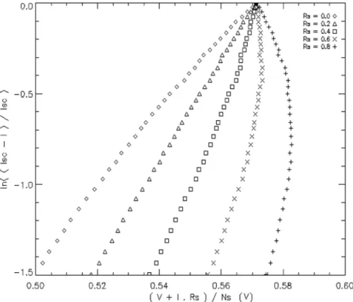
varying Rs in the linearity of the plot of  ln !"#!!_!"# !"  !!!.!!

!! for the selected coordinate points is demonstrated. The plot with Rs = 0.2 Ω shows the result closest to linearity, while the plots with series resistances above 0.2 Ω, curve progressively with the increase of Rs. The same can be said for values lower than 0.2 Ω, thought only one plot with Rs lower than 0.2 Ω is shown.

Figure 13 – Measured I-V curve from a 230 Wp module with 60 cells at 43.3 °C temperature and exposed to 835.41 !/!! _{in-plane irradiance, and the selected I-V coordinate points used for}

the RS and RSH extraction.

Figure 14 – Linear behaviour of the semi-logarithmic plot for different RS values.

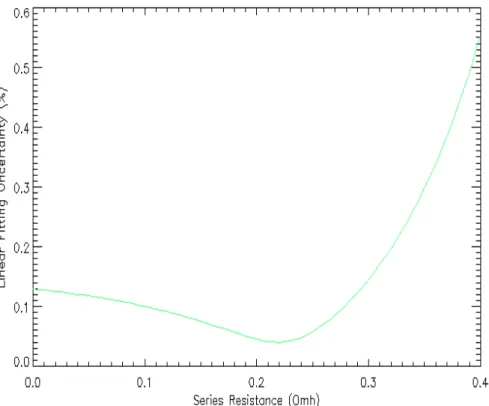
The following figure (Fig. 15) shows the least squares residual uncertainty of the plot as function of RS. The points deviation from a line is higher for RS values further away from the correct one. Thus,

the minimum of the plotted curves coincides with the best estimate for RS. Thus, for this particular

Figure 15 – Linear fitting uncertainty as function of the Series Resistance value used in the semi-logarithmic plot.

After the determination of RS, the parameters I0 and n can be extracted from the intercept and slope of

the line produced with the determined series resistance (see Fig. 16) with Eq. 14. Therefore, for this measured I-V curve, I0 = 4.047E-07 A and n = 1.257.

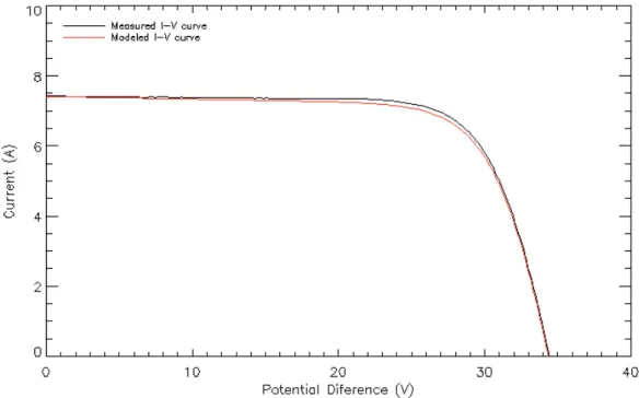
Using the parameters extracted from the I-V curve, and the constants and measured parameters, it is possible to reproduce the measured I-V curve with model calculations, by applying the algorithm mentioned in section 2.2.1 (Eq. 2.9). In Figure 17, both measured and modelled I-V curves are presented.

Figure 17 – Measured I-V curve, and its reproduction using the 1-diode model with the extracted parameters

Observing Figure 17, it can be seen that there is a very small mismatch between the modelled and the measured I-V curve. The mismatch is observed only in the knee part of the I-V curve at high currents and intermediate voltages. The gap can be due to the lack of the 2nd diode in the model equation, as this is the region that the 2nd diode dominates. The key points for both modelled and measured I-V curves are calculated and presented in the following table (Tab. 3).

Table 3 – Key parameters of the measured and reproduced I-V characteristics and their differences

Parameter ISC (A) VOC (V) Peak Power (W) Fill Factor Efficiency (%)

Measured 7.421 34.41 188.54 0.738 13.76

Modelled 7.424 34.41 184.82 0.725 13.49

Difference 0.003 0.00 4.32 - 0.013 - 0.271

The parameter that suffers the most from this mismatch is the max power point, as it is situated on the knee part of the I-V curve, consequently both the fill factor and efficiency are different, as the peak power is one of the inputs for their determination. In the results section, the use of this extraction method is presented for several I-V curves at various temperature and irradiance conditions.