An analysis of the spontaneous mutation rate measurement in filamentous
fungi
Marta S. Baracho and Ivanhoé R. Baracho
Departamento de Genética e Evolução, Universidade Estudual de Campinas, Campinas, SP, Brazil.
Abstract
Mutations related to genemethG1ofAspergillus nidulans were analyzed, in order to study a mathematical model for the determination of the mutation rate per nucleus per generation, in filamentous fungi. A replica plating technique was used to inoculate, in a single operation, 26 colonies of the strain, into Petri dishes containing culture medium, and the nine central colonies were analyzed for size and number of conidia in each colony. Using this technique, several central colonies were analyzed with regard to the appearance of mutation, and the number and type of reversions were determined for each colony. The frequencies obtained for each reversion were analyzed, in order to verify if their distribution was in accordance with that of Greenwood and Yule. The data obtained allowed us to conclude that, using the mathematical model studied, it is possible to determine the mutation rate per nucleus, per generation, in filamentous fungi.
Key words: Aspergillus nidulans, mutation rate, spontaneous mutation, fungi, filamentous fungi.
Received: April 8, 2002; accepted: November 11, 2002.
Introduction
There are two different situations to be taken into ac-count in the determination of spontaneous mutation rates in microorganisms: determination in organisms that grow as free cells, and determination in organisms that grow as my-celia.
Particularly important studies on the first situation concern bacterial populations subject to mutation. The mathematical aspects of this issue started to be considered of greater importance in 1943, when the report of Luria and Delbruck was published, followed by other mathematical studies on this subject, such as the papers by Shapiro (1946), Lea and Coulson (1949), and Armitage (1952, 1953), which gave rise to the development of various meth-ods for the determination of spontaneous mutation rate in organisms that grow as free cells.
However, in organisms that grow as mycelia, the de-termination of the spontaneous mutation rate presents some difficulties, and is usually incomplete. The ideal way of do-ing it would be to determine the mutation probability per nucleus and per generation, as done for bacteria. But, since in filamentous fungi the only easy way of obtaining nucleus samples is through the spores, the usual procedure is to de-termine the proportion of mutants among the spores
formed, without considering whether the mutation oc-curred during spore formation or during previous nuclear divisions.
The objective of the present study was to determine if the Greenwood and Yule distribution (1920) is an adequate mathematical model for the determination of spontaneous mutation rate in filamentous fungi.
Materials and Methods
Media
The minimum medium (MM) used was Czapek-Dox with 1% (w/v) glucose. The complete medium (CM) con-tained yeast extract, hydrolyzed casein, hydrolyzed nucleic acids, vitamins, etc, (Pontecorvoet al., 1953). Solid media contained 2% agar.
Strain
We used the biA1, methG1 strain of Aspergillus
nidulansderived from the Glasgow stock, which was main-tained on complete medium slants at 5 °C. The genetic markers of this strain arebiA1andmethG1,which are a re-quirement, respectively, for biotin and methionine.
Spontaneous mutations
In order to study the mathematical model, spontane-ous mutations related to the genemethG1of A. nidulans
Send correspondence to Marta S. Baracho. E-mail: martbaracho@ hotmail.com.
were analyzed. In a study on this gene, Lilly (1965) ob-served that it was a mutation that could be suppressed by specific suppressor genes not linked to the mutant locus. These revertants appeared spontaneously at a frequency of 1 in 6 x 10⁴conidia, a frequency at least 100 times higher than that observed for other loci. They fall into three visibly distinct types, as follow: type A- colonies which are essen-tially normal; type B- colonies which produce a brown pig-ment in the medium and have sparse conidiation; type C-densely conidiating colonies with hyaline edges.
This methionine system was previously studied by other authors, and different classifications were proposed (Rocha, 1983). However, in the present study the revertants were defined according to the classification of Lilly (1965).
Determination of number of mutants
ThebiA1,methG1strain was inoculated into the cen-ter of Petri dishes measuring 9 cm in diamecen-ter containing 20 mL solid CM, and the preparations were incubated for 9 days at 37 °C. Then, the cultures were replated by means of a 26-needle replicator onto other Petri dishes with CM, and incubated for 4 days. Conidia from each of 9 central colo-nies were suspended in 1 mL Tween 80 solution and shaken for disaggregation. The suspension was filtered through cotton wool into test tubes, and the entire content of the test tubes was spread with a Drigalski spatula onto Petri dishes containing minimum medium supplemented with biotin (0.4µg/mL). The dishes were incubated at 37 °C for 10 days, and then the number and type of colonies that arose were determined.
Determination of colony size and number of conidia per colony
Central colonies obtained as described above were mea-sured with a millimeter ruler to determine their diameter and variation. Conidial suspensions obtained from these colonies and treated as described above were counted with a hemo-cytometer, to estimate the number of conidia per colony.
Determination of conidial viability
Conidia from colonies allowed to grow in CM for 4 days were placed in Tween 80 solution, disaggregated by shaking, and counted with a hemocytometer. The conidial suspensions were then diluted in saline solution, in order to obtain appropriate numbers for seeding. 0.1 mL aliquots of this diluted conidial suspension were seeded on Petri dishes containing CM, and spread with a Drigalski spatula. The dishes were incubated for 2 days, and the number of grow-ing colonies was counted.
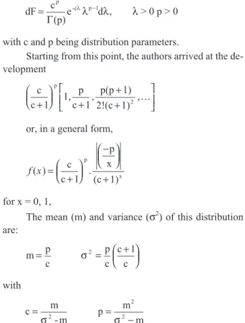
Mathematical model
In the present study, we considered Greenwood and Yule’s distribution (1920) as the onset model of mutant
conidia generated by nuclei that underwent the mutation. These authors, when referring to the number of accidents, assumed that their distribution was of the Poisson type,
f(j) e j!
j
= −λ λ
for j = 0, 1, ..., withλbeing a random variable which ex-presses the distinct degrees of individual risk to which the population is subject, and whose distribution function is given by:
dF c
(p)e d
p
-c p 1
= −
Γ
λλ λ, λ> 0 p > 0
with c and p being distribution parameters.
Starting from this point, the authors arrived at the de-velopment
c c 1 1,
p c 1,
p(p 1) 2!(c 1)
p
2
+
+
+ +
,K
or, in a general form,
f x( )= .
+
−
+
c c 1
p x (c 1)
p
x
for x = 0, 1,
The mean (m) and variance (σ2) of this distribution are:
m p c
= σ2 = +
p c
c 1 c
with
c m
- m
2
=
σ p
m m
2 2
= − σ
Although Greenwood and Yule (1920) studied mainly the occurrence of accidents, considering the differ-ent degrees of individual risks, the application of their dis-tribution to the study of mutations proposed here can be easily justified. It is enough to consider the occurrence of mutant conidia in view of the distinct possibilities of the ap-pearance of nuclei where a mutation took place.
Results
Number of mutants
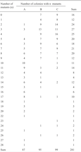
Table 1 shows the frequencies of type A, B, and C re-versions for each colony obtained from strainbiA1,methG1 by the technique described above.
distribu-tion. The mean number of nuclei where a mutation took place was obtained by the following formula:
p m
m
2 2
= − σ
For type A reversions, we examined 87 colonies, which presented a mean number of 12.30 mutants per col-ony, and a variance of 28.54. The mean number of nuclei where a mutation took place was 9.31. For type B rever-sions, we examined 95 colonies, which presented a mean number of 6.17 mutants, and a variance of 23.45. The mean number of nuclei where a mutation took place was 2.21. For type C reversions, we examined 99 colonies, which pre-sented a mean number of 4.97 mutants per colony, and a
variance of 22.34. The mean number of nuclei where a mu-tation took place was 1.42.
Conidial viability
Conidial viability was determined by hemocytometer counting, and the rates obtained were, respectively, 87% vi-able conidia for strainbiA1,methG1, 100% for the type A reversion, 83% for the type B reversion, and 71% for type C reversions.
Colony size and number of conidia per colony
Fifty-four central colonies of the strainbiA1,methG1 obtained as described earlier were measured, and their di-ameter was found to range from 11 to 14 mm, with a mean and standard error of the mean of 11.89 ± 0.12. The number of conidia of these 9 colonies was estimated by hemocytometer counting, and the mean detected was 3.8 x 10⁷± 6.1 x 10⁶conidia per colony.
Discussion
Frequency of mutants
Three types of phenotypically distinguishable rever-sions of themethG1gene were studied. The number of mu-tants detected in each colony is listed in Table 1.
Several studies using the same strain (originated in Glasgow, UK) to detect the mutagenic activity of physical and chemical agents have reported results referring to these spontaneous reversions. Siddiqui (1962) reported a sponta-neous mutation frequency of about 8.2 x 10⁻⁶, with 34.2% for type A, 31.2% for type B, and 35% for Type C, respec-tively.
Lilly (1965) reported a frequency of 1 in 6 x 10⁴, which is approximately 17 x 10-6, with rates of 66% for Type A, 31% for type B, and 3% for Type C, respectively. Alderson and Clark (1966) conducted two experiments. In one of them, they detected frequencies of 9.2 x 10⁻⁶, with a distribution of 35% for Type A, 65% for Type B, and 0% for Type C. In the other experiment, the frequency was 1.1 x 10⁻⁶, with a distribution of 63% for Type A, 29% for Type B, and 8% for Type C. In contrast, data reported by Duarte (1972) showed a frequency of 12.6 x 10⁻⁶, with a distribution of 58% for Type A, 31% for Type B, and 11% for Type C. Scott et al. (1973) reported frequencies of 2 x 10⁻⁶to 5 x 10⁻⁶, while Rocha (1983) detected variations from 6.4 x 10⁻⁶to 20.4 x 10⁻⁶.
In the present study, we detected a frequency of 0.95 x 10⁻⁶(approximately 1 x 10⁻⁶), with a proportion of 61% for Type A, 25% for Type B, and 14% for Type C.
Thus, the data reported by the various authors are dis-crepant. However, in the present study we determined the number of mutants per colony and estimated the number of conidia in each colony, whereas in the other studies the Table 1- Frequencies observed for type A, B, and C reversions.
Number of mutants (n)
Number of colonies with n mutants
A B C Sum
0 7 9 16
1 4 8 12
2 1 9 14 24
3 3 13 11 27
4 9 16 25
5 4 7 9 20
6 3 9 6 18
7 5 7 9 21
8 6 7 7 20
9 4 7 1 12
10 10 1 11
11 9 3 2 14
12 4 4 8
13 3 1 4
14 6 4 2 12
15 3 1 4
16 6 6
17 8 1 1 10
18 1 1
19 5 5
20 2 2
22 1 1
23 1 1
24 1 1 2
25 1 1
26 1 1 2
27 1 1
28 1 1
number of conidia was estimated in a suspension, and a known volume of this suspension was used to determine the number of mutants that arose.
Mean number of nuclei that underwent a mutation
The frequency of mutant conidia does not provide an actual idea of the number of mutations that actually oc-curred, since, in the case of Aspergillus nidulans, the conidia are formed from secondary sterigmas by repeated nuclear division. The conidia start to develop as cytoplas-mic protuberances at the end of the sterigmas. The nucleus of the sterigma then undergoes one mitotic division and, while one of the two resulting nuclei enters the region that will be transformed into a conidium, the other moves to the opposite end. As the conidium becomes delimited, the nu-cleus of the sterigma starts to divide again, to produce an-other conidium. The process thus continues, with the formation of a long chain in which the last conidium formed is closest to the sterigma, while the conidium that was first formed is the most distant one (Timberlake, 1990). In view of this formation process, it is clear that the number of mutant conidia in a chain will depend on the mo-ment when the mutation occurred in the nucleus of the sterigma. If the mutation occurred long before sterigma for-mation, obviously an entire conidial head may be mutated. Therefore, the frequency of mutant conidia does not corre-spond to the frequency of mutations that actually occurred per nucleus, and consequently the mutation rate cannot be determined on this basis.
As pointed out by Fincham and Day (1971), the ideal in this case would be “to measure the chance of mutation occurring per nucleus per time unit, or per nuclear genera-tion time.” This is possible in organisms that grow as free cells. In filamentous fungi, however, a nucleus sample is easily obtained only by using spores, which makes it diffi-cult to determine the mutation rate. Usually, what is deter-mined is the frequency of mutating spores.
This is what is commonly done in mutation studies with thebiA1methG1strain. In this case, the nucleus sam-ples come from conidial samsam-ples in which, as mentioned earlier, the number of mutant nuclei does not correspond to the number of nuclei that underwent mutation. Therefore, a mathematical model has to be established that permits to estimate the number of nuclei that underwent mutation based on the number of mutant conidia, like the distribution of Greenwood and Yule.
The model
Frequencies were calculated for a theoretical distribu-tion (Greenwood and Yule distribudistribu-tion) and for the sam-pling data referring to Type A, B, and C reversions, and an adherence test was performed to determine whether the fit of the data observed to the theoretical distribution chosen
was good. The adherence test used was the Kolmogorov--Smirnov test, used to determine whether the observed accumulated frequency departs significantly from a hy-pothesized frequency distribution. The point where these two distributions - theoretical and observed - show the greatest divergence is determined, and this maximum ob-served deviation (D) is compared to a tabled value, to deter-mine if it is too large to be attributed to chance (Siegel, 1975).
Thus, the Kolmogorov-Smirnov test can demonstrate if the mathematical model chosen serves the purpose of the study, which in our case was the capacity to estimate the mean number of nuclei that underwent mutation based on the number of mutant conidia, with a consequent estimate of the mutation rate per nucleus per generation.
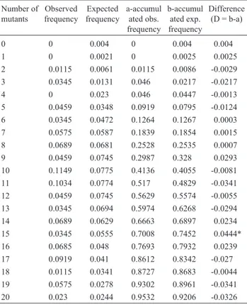
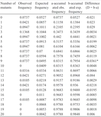
The result of the Kolmogorov-Smirnov test for Type A reversions can be seen in Table 2. A D value of 0.0444, non-significant at the 5% level of probability, was detected, thus indicating that the Greenwood and Yule distribution fits the data. The results concerning Type B reversions are listed in Table 3. In this case, the value of D was 0.0361, also non-significant at the 5% level of probability. For Type C reversions, the results are presented in Table 4, which shows a value of D = 0.0877, non-significant at the 5% level as well.
Table 2- Determination of the goodness of fit of the frequencies observed for type A reversions (Table 1) to the theoretical frequencies of the Greenwood-Yule distribution (Kolmogorov-Smirnov test).
Number of mutants
Observed frequency
Expected frequency
a-accumul ated obs. frequency
b-accumul ated exp. frequency
Difference (D = b-a)
0 0 0.004 0 0.004 0.004
1 0 0.0021 0 0.0025 0.0025
2 0.0115 0.0061 0.0115 0.0086 -0.0029 3 0.0345 0.0131 0.046 0.0217 -0.0217 4 0 0.023 0.046 0.0447 -0.0013 5 0.0459 0.0348 0.0919 0.0795 -0.0124 6 0.0345 0.0472 0.1264 0.1267 0.0003 7 0.0575 0.0587 0.1839 0.1854 0.0015 8 0.0689 0.0681 0.2528 0.2535 0.0007 9 0.0459 0.0745 0.2987 0.328 0.0293 10 0.1149 0.0775 0.4136 0.4055 -0.0081 11 0.1034 0.0774 0.517 0.4829 -0.0341 12 0.0459 0.0745 0.5629 0.5574 -0.0055 13 0.0345 0.0694 0.5974 0.6268 -0.0294 14 0.0689 0.0629 0.6663 0.6897 0.0234 15 0.0345 0.0555 0.7008 0.7452 0.0444* 16 0.0685 0.048 0.7693 0.7932 0.0239 17 0.0919 0.041 0.8612 0.8342 -0.027 18 0.0115 0.0341 0.8727 0.8683 -0.0044 19 0.0575 0.0278 0.9302 0.8961 -0.0341 20 0.023 0.0244 0.9532 0.9206 -0.0326
The sampling frequencies of the three types of rever-sions, therefore, fit the theoretical frequencies of Green-wood and Yule’s distribution. Consequently, it is valid to use this distribution to calculate the mean number of mu-tated nuclei based on the number of mutant conidia. This estimate definitely permits the calculation of the mutation rate per nucleus per generation, when the data concern a single gene.
Acknowledgments
This work was supported by Capes.
References
Alderson T and Clark AM (1966) Interlocus specificity for chemi-cal mutagens inAspergillus nidulans. Nature 210:593-595. Armitage P (1952).The statistical theory of bacterial populations
subject to mutation. Journal of Royal Statistical Society 14:1.
Armitage P (1953) Statistical concepts in the theory of bacterial mutation. Journal of Hygiene 51:162-183.
Duarte FM (1971) Efeitos mutagênicos de alguns ésteres de ácidos inorgânicos em Aspergillus nidulans. Ciência e Cultura 24:42-52.
Fincham JRS and Day PR (1971) Fungal Genetics. Botanical Monographs, v. 4, Blackwell Scientific Publications. Phila-delphia, Pennsylvania.
Greenwood M and Yule GU (1920) An enquiry into the nature of frequency distributions representative of multiple happen-ings with particular reference of multiple attacks of disease or of repeated accidents. Journal Royal Statistical Society 83:255-279.
Lea DE and Coulson CA (1949) The distribution of the numbers of mutants in bacterial populations. Journal of Genetics 49:264-285.
Lilly JL (1965) An investigation of the suitability of the suppressors of meth1 inAspergillus nidulansfor study of induced and spontaneous mutation. Mutation Research 2:192-195. Luria SE and Delbruck M (1943) Mutations of bacteria from virus
sensitivity to virus resistance. Genetics 28:491-511. Pontecorvo G, Roper JA, Hemmons LM, MacDonald KD and
Bufton AW (1953) The genetics of Aspergillus nidulans. Advances in Genetics 5:141-238.
Rocha CLMSC (1983) Detecção da atividade mutagênica de produtos químicos no sistema meth1 emA. nidulans. Tese de Mestrado, pp 77.
Scott BR, Alderson T and Papworth DG (1973) The effect of plat-ing densities on the retrieval of methionine suppressor muta-tion after ultraviolet or gamma irradiamuta-tion of Aspergillus. Journal of General Microbiology 75:235-239.
Shapiro A (1946) The kinetics of growth and mutation in bacteria. Cold Spring Harbor Symposia on Quantitative Biology 11:228.
Siddiqui OH (1962) Mutagenic action of nitrous acid on Aspergillus nidulans. Genetical Research 3:303-314. Siegel S (1975) Estatística não-paramétrica. Editora Mcgraw-Hill
do Brasil, São Paulo, pp 332.
Timberlake WE (1990) Molecular genetics ofAspergillus devel-opment. Annual Review Genetics 24:5-36.
Associate Editor: Darcy Fontoura de Almeida Table 3- Determination of the goodness of fit of the frequencies observed
for type B reversions (Table 1) to the theoretical frequencies of the Greenwood-Yule distribution (Kolmogorov-Smirnov test).
Number of mutants
Observed frequency
Expected frequency
a-accumul ated obs. frequency
b-accumul ated exp. frequency
Difference (D = b-a)
0 0.0737 0.0527 0.0737 0.0527 -0.021 1 0.0421 0.0857 0.1158 0.1384 0.023 2 0.0947 0.1011 0.2105 0.2395 0.029 3 0.1368 0.1044 0.3473 0.3439 -0.0034 4 0.0947 0.1002 0.442 0.4441 -0.0021 5 0.0737 0.0913 0.5157 0.5356 0.0199 6 0.0947 0.081 0.6104 0.6166 -0.0062 7 0.0737 0.07 0.6841 0.6866 0.0025 8 0.0737 0.0594 0.7578 0.7459 -0.0119 9 0.0737 0.0495 0.8315 0.7954 -0.0361* 10 0 0.0409 0.8315 0.8363 0.0048 11 0.0316 0.0334 0.8631 0.8697 0.0066 12 0.0421 0.0271 0.9052 0.8968 -0.084 13 0.0105 0.0218 0.9157 0.9186 0.0029 14 0.0421 0.0174 0.9578 0.936 -0.0218 15 0.0105 0.0128 0.9683 0.9488 -0.0195 16 0 0.011 0.9683 0.9598 -0.0085 17 0.0105 0.0087 0.9783 0.9685 -0.0098 18 0 0.0068 0.9788 0.9753 -0.0035 19 0 0.0053 0.9788 0.9806 0.0018 20 0 0.0042 0.9788 0.9848 0.006
*D = 0,0361 – Non-significant at the 5% level of probability.
Table 4- Determination of the goodness of fit of the frequencies observed for type C reversions (Table 1) to the theoretical frequencies of the Greenwood-Yule distribution (Kolmogorov-Smirnov test).
Number of mutants
Observed frequency
Expected frequency
a-accumul ated obs. frequency
b-accumul ated exp. frequency
Difference (D = b-a)
0 0.0909 0.1179 0.0909 0.1179 0.027 1 0.0808 0.1304 0.1717 0.2484 0.0767 2 0.1414 0.1228 0.3131 0.3712 0.0581 3 0.1111 0.1033 0.4242 0.4746 0.0504 4 0.1616 0.0936 0.5858 0.5682 -0.0176 5 0.0909 0.0789 0.6767 0.6472 0.0295 6 0.0606 0.0656 0.7373 0.7129 -0.0245 7 0.0909 0.0541 0.8282 0.7669 -0.0613 8 0.0707 0.0443 0.8989 0.8112 -0.0877* 9 0.0101 0.0360 0.909 0.8472 -0.0618 10 0.0101 0.0292 0.9191 0.8764 -0.0427 11 0.0202 0.0236 0.9393 0.9 -0.0393 12 0 0.0190 0.9393 0.9119 -0.0274 13 0 0.0152 0.9393 0.9271 0.0122 14 0.0202 0.0122 0.9595 0.9393 0.0202 15 0 0.0098 0.9595 0.9491 0.0104 16 0 0.0078 0.9595 0.9569 0.0026 17 0.0101 0.0062 0.9696 0.9631 0.0065 18 0 0.0049 0.9696 0.968 0.0016 19 0 0.0039 0.9696 0.9719 0.0023 20 0 0.0031 0.9696 0.975 0.0054