WRF simulation of a precipitation event over the Tibetan Plateau, China – an assessment using remote sensing and ground observations

(1)

www.hydrol-earth-syst-sci.net/15/1795/2011/ doi:10.5194/hess-15-1795-2011

Earth System

Sciences

WRF simulation of a precipitation event over the Tibetan Plateau,

China – an assessment using remote sensing and ground

observations

F. Maussion1, D. Scherer1, R. Finkelnburg1, J. Richters1, W. Yang2, and T. Yao2

1_{Institut f¨ur ¨}_{Okologie, Technische Universit¨at Berlin, 12165 Berlin, Germany}

2_{Institute of Tibetan Plateau Research, Chinese Academy of Sciences (CAS), Beijing 100085, China}

Received: 30 May 2010 – Published in Hydrol. Earth Syst. Sci. Discuss.: 16 June 2010 Revised: 21 March 2011 – Accepted: 22 May 2011 – Published: 10 June 2011

Abstract. Meteorological observations over the Tibetan Plateau (TiP) are scarce, and precipitation estimations over this remote region are difficult. The constantly improving ca-pabilities of numerical weather prediction (NWP) models of-fer the opportunity to reduce this problem by providing pre-cipitation fields and other meteorological variables of high spatial and temporal resolution. Longer time periods of years to decades can be simulated by NWP models by successive model runs of shorter periods, which can be described by the term “regional atmospheric reanalysis”. In this paper, we as-sess the Weather Research and Forecasting (WRF) models capacity in retrieving rain- and snowfall on the TiP in such a configuration using a nested approach: the simulations are conducted with three nested domains at spatial resolutions of 30, 10, and 2 km. A validation study is carried out for a one-month period with a special focus on one-week (22– 28 October 2008), during which strong rain- and snowfall was observed on the TiP. The output of the model in each resolution is compared to the Tropical Rainfall Measuring Mission (TRMM) data set for precipitation and to the Moder-ate Resolution Imaging Spectroradiometer (MODIS) data set for snow extent. TRMM and WRF data are then compared to weather-station measurements. Our results suggest an over-all improvement from WRF over TRMM with respect to weather-station measurements. Various configurations of the model with different nesting and forcing strategies, as well as physical parameterisation schemes are compared to propose a suitable design for a regional atmospheric reanalysis over the TiP. The WRF model showed good accuracy in simulat-ing snow- and rainfall on the TiP for a one-month simulation period. Our study reveals that there is nothing like an optimal

Correspondence to:F. Maussion (fabien.maussion@tu-berlin.de)

model strategy applicable for the high-altitude TiP, its fring-ing high-mountain areas of extremely complex topography and the low-altitude land and sea regions from which much of the precipitation on the TiP is originating. The choice of the physical parameterisation scheme will thus be always a compromise depending on the specific purpose of a model simulation. Our study demonstrates the high importance of orographic precipitation, but the problem of the orographic bias remains unsolved since reliable observational data are still missing. The results are relevant for anyone interested in carrying out a regional atmospheric reanalysis. Many hy-drological analyses and applications like rainfall-runoff mod-elling or the analysis of flood events require precipitation rates at daily or even hourly intervals. Thus, our study of-fers a process-oriented alternative for retrieving precipitation fields of high spatio-temporal resolution in regions like the TiP, where other data sources are limited.

1 Introduction

The Tibetan Plateau (TiP) is the source of many major rivers in Central Asia, thus affecting hundreds of millions of peo-ple in the surrounding regions. Its glaciers are characteris-tic elements of the natural environment, forming water re-sources of great importance for both ecosystems and local population. Yao et al. (2007) underlined the importance of the Tibetan and Himalayan glaciers on the hydrological ditions in Asia. Several studies have shown the strong con-trol of orography and boundary-layer structure of the TiP on the Asian monsoon system (e.g., Gao et al., 1981; Hahn and Manabe, 1975).

(2)

Forschungsgemeinschaft (DFG) to develop a multidisci-plinary approach dealing with the complex processes and in-teractions taking place between the major driving forces on the TiP. This study took place within this frame.

Located in a transition zone between the continental cli-mate of Central Asia and the Indian Monsoon system, the Nam Co drainage basin including the western Nyainqentan-glha Mountains has been pointed out as a key research area in Tibet, and is also investigated in this study. The recent rise of the lake level of Nam Co, one of the largest and highest lakes on the TiP (year 2000: 1980 km2area, 4724 m a.s.l. lake level altitude), has been attributed to glacier retreat as well as to an increase of precipitation in recent decades (e.g., Wu and Zhu, 2008; Krause et al., 2010). Precipitation increase in central TiP during this period has also been reported by Liu et al. (2009). However, the TiP remains a sparsely ob-served region, and there is limited availability of meteoro-logical data. This is especially true for long-term weather records necessary for reliable climatological studies (Frauen-feld et al., 2005; Kang et al., 2010). In particular, no long-term data from weather stations are existing at elevations above 4800 m a.s.l. Generally, the geographical distribution of weather stations is biased towards lower altitudes, flat ar-eas and specific land-cover types excluding high-mountain regions covered by glaciers. The question of the respective contributions of glacier retreat and precipitation increase to rising lake levels on the TiP remains unanswered, so far, for these reasons.

Besides air temperature, precipitation is considered to be a key variable for understanding recent environmental vari-ability and trends on the TiP. Unfortunately, precipitation is strongly influenced by terrain, and can hardly be retrieved from existing gridded precipitation data sets, especially in mountainous regions. This has been discussed e.g. by Yin et al. (2008) for problems in using remotely sensed precipi-tation data sets derived from the Tropical Rainfall Measuring Mission (TRMM), and also for global atmospheric reanalysis data (e.g., Ma et al., 2009).

The constantly improving capabilities of numerical weather prediction (NWP) models offer the opportunity to reduce this problem by providing precipitation fields and other meteorological variables at high spatial and temporal resolution. Generally, NWP models are suitable not only for weather forecasting but also for dynamical downscaling of large-scale atmospheric processes. NWP models can be ini-tialised and laterally forced by assimilated observational data describing the large-scale atmospheric conditions throughout the simulation period, thus keeping the model results close to observations also at finer spatial scales. This approach enables validation of the model output for single events but does not allow forecasts, since the assimilated observational data have to be available not only for the time of model ini-tialisation but for the whole simulation period.

Longer time periods of years to decades can be simulated by NWP models by successive model runs of shorter periods

of time integration of days to weeks. We will subsequently use the term “regional atmospheric reanalysis” for this kind of NWP-model application. A good example of a regional at-mospheric reanalysis is given by Box et al. (2004) who used the Atmospheric Research Mesoscale Model MM5 for gen-erating a contiguous multi-year weather data set for Green-land by dynamical downscaling of 2.5◦

operational analyses from the European Centre for Medium-Range Weather Fore-casts (ECMWF) by a sequence of daily model runs. Box et al. (2006) used the MM5 output for driving a surface mass balance model of the Greenland Ice Sheet.

Caldwell et al. (2009) simulated the climate of Califor-nia for a 40 yr period by the Weather Research and Forecast-ing (WRF) model, which has been re-initialised every month. The latter simulation is, however, not driven by assimilated observational data but by the output of a General Circula-tion Model (GCM), which makes it impossible to validate the model results also on an event-basis. Dynamical down-scaling of GCM simulations required for climate reconstruc-tions or projecreconstruc-tions could also be done by Regional Climate Models (RCM). Lo et al. (2008), for example, discussed dif-ferent strategies for time integration. Fowler et al. (2007) and Laprise et al. (2008) presented in-depth discussions of approaches and challenges including e.g. hydrological appli-cations.

The approach of Box et al. (2004) is of special interest also for the TiP. However, the capacity of the models in re-trieving snow- and rainfall in complex terrain is still dis-cussed. Using higher horizontal spatial resolution of less than 10 km has been advanced as a substantial improve-ment, as it allows more accurate representation of mountain regions. Mountain-valley structures in the Nyainqentanglha Mountains are often showing elevation differences of 1 to 2 km within short distances of less than 10 km, which is com-mon for high-mountain regions all over the world. Zaengl (2007) shows that increased spatial resolutions in areas of complex terrain can be highly beneficial for simulating pre-cipitation fields. However, higher spatial resolution does not automatically improve a NWP models skill in predicting pre-cipitation in mountainous regions. Studies like the one from Zaengl (2007) have shown that increasing the spatial reso-lution does not improve the model quality for precipitation caused by embedded convection.

(3)

80E 90E 100E 10N

20N 30N 40N

85E 90E 95E

25N 30N 35N

Baingoin

Dege Dengqen

Deqen Lhasa

Lhunze

Madoi

Nagqu

Nyingchi

Pagri

Qamdo Qumarleb

Sog_xian

Tingri

Tuotuohe

Xainza

Xigaze

Yushu Zadoi

Namco

90E 91E 92E

30N 31N 32N

Baingoin

Lhasa

Nagqu

Namco

Water 0 250 650 1000 1400 1800 2200 2600 3000 3400 3800 4200 4600 5000 5400 5800 Alt. (m a.s.l.)

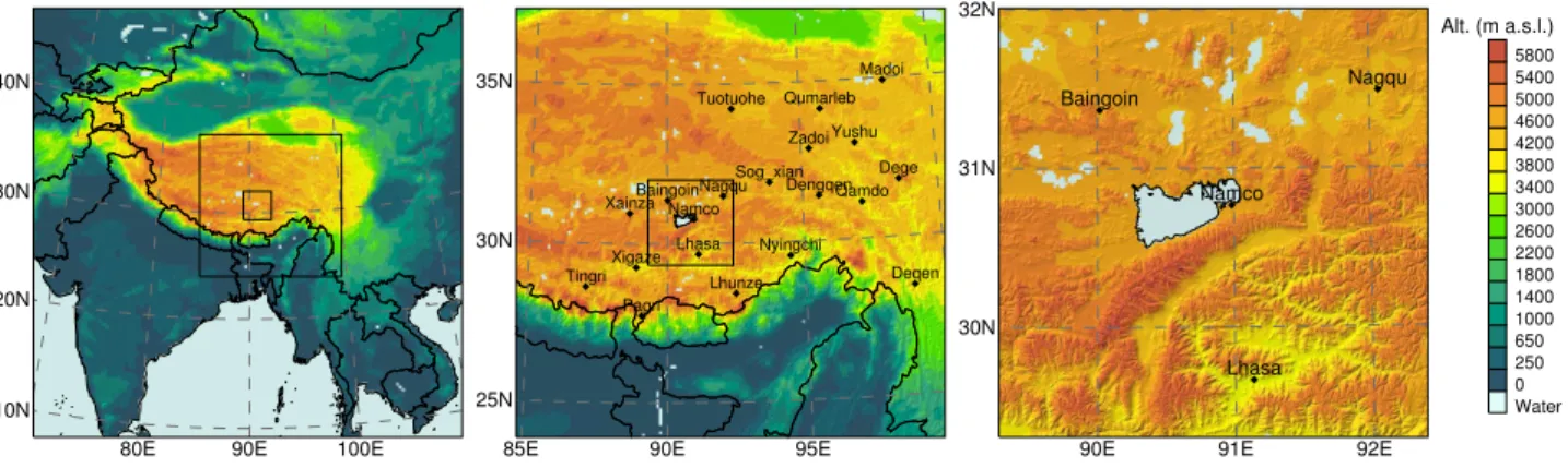
Fig. 1. WRF domains and model topography. Left: large domain (LD); the medium (MD) and small (SD) are indicated by black frames. Center: medium domain. Right: small domain. Black dots represent the locations of the available weather stations.

in high-mountain drainage basins, prerequisite to subsequent hydrological studies.

Only few studies employed the Weather Research and Forecasting (WRF) model on the TiP, by that time. Li et al. (2009) investigated the sensitivity of the WRF model to sur-face skin temperature of Nam Co for simulating a precipita-tion event. Sato et al. (2008) analysed the sensitivity of the WRF model to horizontal grid spacing with respect to sim-ulate the diurnal cycle of precipitation. Their results show that the finest spatial resolution (7 km) is more efficient in representing diurnal cloud formation than coarser grids. So far, no study used the WRF model for a regional atmospheric reanalysis.

1.1 Objectives

The main objective of our study is optimising the design of a modelling strategy including a suitable model configura-tion for producing a weather data set of high spatio-temporal resolution for the study region by a regional atmospheric re-analysis. This is particularly relevant for subsequent hydro-logical and glaciohydro-logical studies, e.g. requiring detailed pre-cipitation fields as input data in hydrological and glaciolog-ical models. In this paper, we therefore concentrate on the capacity of the WRF model in retrieving data on solid and liquid precipitation. For this purpose, we focus on a specific precipitation event over the TiP (see Sect. 1.3) including its contribution to monthly precipitation amounts.

While dynamical downscaling studies employing RCM use integration periods from months to years or even many decades, the objective of our study is to analyse the capabil-ity of the WRF model as a NWP model to be employed for a regional atmospheric reanalysis, enabling direct compari-son of model results with observations. By using a contin-uous sequence of short time integration periods, we prevent the model deviating too much from large-scale observations. After two days of simulation we expect the model to be less accurate than during the first two days. Therefore, our study

also aims at a quantitative analysis of the effects of using dif-ferent strategies for time integration.

In this study, we address two main research questions: 1. Which validation methods and data sets are suitable for

assessing the accuracy of simulated precipitation fields of high spatio-temporal resolution over the TiP? 2. Is a specific set-up of the WRF model able to

reanal-yse precipitation fields in the mountainous and sparsely observed region of the TiP?

The first question is less frequently addressed in similar model studies since observations are usually taken as an ab-solute reference to assess the performance of a model. How-ever, the particularities of the TiP do not ensure the applica-bility of validation approaches that have been proven to be suitable in other regions. Especially without knowing the limitations of the validation data sets the second question may not be answered appropriately.

The WRF model, like other NWP models, offers a broad spectrum of options for setting up and forcing simulations, including various parameterisation schemes for sub-scale processes. We present a sensitivity study following the gen-eral ideas as discussed e.g. by Rakesh et al. (2007) or Yang and Tung (2003) to quantify the uncertainty in the model out-put caused by the model itself.

(4)

0 50 100 150 Number of days

0 20 40 60 80 100

Contribution to annual precipitation (%)

0 50 100 150

Number of days 0

20 40 60 80 100

Contribution to annual precipitation (%)

11 32

50

Fig. 2. Contribution (%) of accumulated daily precipitation to the annual precipitation in the year 2008 for the 19 available weather stations. The daily precipitation values are sorted in decreasing or-der. The number of days in which 50 % of the annual precipitation is reached are indicated for the two extremal stations.

1.2 Study region

The study region and the set-up of the three nested domains used by the WRF model are presented in Fig. 1.

The large domain (LD) covering an area of 4500×4500 km2 is used to capture large-scale processes and to avoid model artefacts near the lateral boundaries. The studied precipitation event originated from the Bay of Bengal, which is fully covered by the LD.

The medium domain (MD) covers an area of 1500×1500 km2comprising large parts of the TiP including the western and eastern Nyainqentanglha Mountains. The southern-eastern part of the TiP is strongly influenced by the summer monsoon, and has generally lower altitudes, thus maritime (temperate) glaciers are present, while glaciers in the central, northern and western parts of the TiP are mostly continental (cold or polythermal) (see Shi and Liu, 2000, for a detailed description).

Detailed analyses are carried out for the small domain (SD) covering an area of 300×300 km2. The SD is cen-tred on Nam Co and its drainage basin. The highly glaciated western Nyainqentanglha Mountains (see Bolch et al., 2010), reaching elevations of more than 7100 m a.s.l., are fully contained in the SD. Nam Co and the other lakes sig-nificantly influence local climates and atmospheric mois-ture content (Haginoya et al., 2009). The presence of the well-equipped Nam Co Monitoring and Research Sta-tion (30◦

46′

N, 90◦

59′

E, 4730 m a.s.l., located in the south-eastern shore of the lake; see Fig. 1), operated by the Institute of Tibetan Plateau Research (ITP) of the Chinese Academy

of Sciences (CAS), makes it one of the most intensively stud-ied regions on the TiP, and thus an ideal test bed for our study. 1.3 Simulation period

Focusing model-validation studies on short simulation pe-riods enlightens some particularities and issues that are not visible in long-term validation studies. Short-term validation studies enable evaluation of precipitation rates and cumu-lated amounts on a process-oriented basis. Individual strong precipitation events are well suited for this kind of analysis, also due to the fact that relative errors in simulated precipi-tation are generally larger in these cases, and thus easier to detect and quantify.

The complex terrain of the high-mountain fringe of the TiP and its blocking effect on moisture transfer coming from the Indian and Pacific Oceans has a characteristic impact on the formation of orographically induced storms (Chen et al., 2007) causing strong precipitation events. The tropical cy-clone Rashmi formed in the Bay of Bengal on 24 Octo-ber 2008, reaching the coast on late evening of 26 OctoOcto-ber. Strong winds and heavy rainfall occurred over Bangladesh and India causing substantial damages and fatalities (the In-dia Meteorological Department made a comprehensive de-scription of the event in IMD, 2008). The system weakened rapidly after landfall, carrying along further precipitation, mainly as snowfall, on the Himalayas and the TiP. This pre-cipitation event happened after the monsoon period, and is challenging the model by its complexity: cyclonal formation overseas and snowfall over the TiP.

On 27 October 2008 daily precipitation amount averaged over the 19 operational weather stations used in our study (see Sect. 2.4) is the absolute maximum of the last decade. The event was also one of the strongest snowfall events in the autumn season affecting large areas on the TiP that have been snow-free prior to the event, which allows a quantitative analysis of the simulated snowfall. Thus, October 2008 was chosen for the study as simulation period. A one-week pe-riod between 22 and 28 October 2008 was used for detailed analysis of the precipitation event.

(5)

(Deqen), but some of the stations far away from the cyclone track (see Sect. 3) showed almost no precipitation at the same time.

2 Methodology

2.1 Design of the reference experiment

The NWP model used in this study is the community WRF-ARW model, version 3.1.1, developed primarily at the Na-tional Center for Atmospheric Research (NCAR) in collabo-ration with different agencies like the National Oceanic and Atmospheric Administration (NOAA), the National Center for Environmental Prediction (NCEP), and many others. The WRF is a limited-area, non-hydrostatic, primitive-equation model with multiple options for various physical parameter-isation schemes (Skamarock et al., 2008).

The three nested domains described in Sect. 1.2 and dis-played in Fig. 1 are used in all the experiments of this study. Spatial resolutions of the different model grids covering the three WRF domains are 30 km for the LD grid, 30 and 10 km for the two MD grids, as well as 30, 10 and 2 km for the three SD grids. WRF model output in the three different spa-tial resolutions (30, 10 and 2 km) will be named WRF30, WRF10 and WRF2 to avoid confusions between model do-mains and spatial resolutions (e.g. WRF30-SD indicates the WRF results for the 30 km grid of the SD).

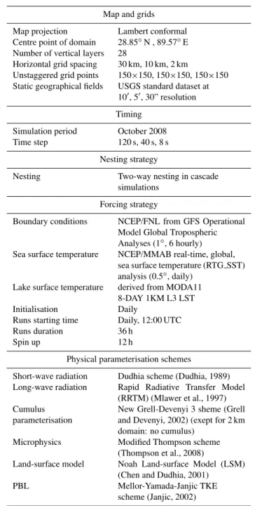
We have designed a reference experiment against which a series of further experiments are performed and analysed to understand how and why simulated precipitation fields change with modified nesting and forcing strategies, as well as with modified physical parameterisation schemes. The de-sign of the reference experiment is resumed in Table 1. The choices for the design of the reference experiments have been following three principles:

1. The reference experiment should incorporate expe-rience gained from comparable numerical modelling studies as far as possible, such that its design is expected to be one of the most suitable candidates for a decadal regional atmospheric reanalysis.

2. The nesting and forcing strategy of the reference ex-periment shall not only enable reanalysing precipita-tion fields but also be suitable for further model ex-periments, e.g. for simulations using modified boundary conditions.

3. The reference experiment shall preserve the predictive skill of the model providing the large-scale forcing fields while concurrently allowing the WRF model to utilise its predictive skills at the resolved scales. The nesting strategy of the reference experiment is based on a novel method, solving a scientific conflict currently dis-cussed concerning the advantages and disadvantages of

one-Table 1.Design of the reference experiment (RE).

Map and grids

Map projection Lambert conformal

Centre point of domain 28.85◦_{N , 89.57}◦_E

Number of vertical layers 28

Horizontal grid spacing 30 km, 10 km, 2 km

Unstaggered grid points 150×150, 150×150, 150×150 Static geographical fields USGS standard dataset at

10′_{, 5}′_{, 30” resolution}

Timing

Simulation period October 2008

Time step 120 s, 40 s, 8 s

Nesting strategy

Nesting Two-way nesting in cascade

simulations

Forcing strategy

Boundary conditions NCEP/FNL from GFS Operational

Model Global Tropospheric Analyses (1◦_{, 6 hourly)}

Sea surface temperature NCEP/MMAB real-time, global, sea surface temperature (RTG SST) analysis (0.5◦_{, daily)}

Lake surface temperature derived from MODA11 8-DAY 1KM L3 LST

Initialisation Daily

Runs starting time Daily, 12:00 UTC

Runs duration 36 h

Spin up 12 h

Physical parameterisation schemes

Short-wave radiation Dudhia scheme (Dudhia, 1989)

Long-wave radiation Rapid Radiative Transfer Model

(RRTM) (Mlawer et al., 1997) Cumulus

parameterisation

New Grell-Devenyi 3 sheme (Grell and Devenyi, 2002) (exept for 2 km domain: no cumulus)

Microphysics Modified Thompson scheme

(Thompson et al., 2008)

Land-surface model Noah Land-surface Model (LSM)

(Chen and Dudhia, 2001)

PBL Mellor-Yamada-Janjic TKE

scheme (Janjic, 2002)

way versus two-way nesting. Some authors (Harris and Dur-ran, 2010) argue that two-way nesting increases the predic-tive skill of a NWP model within the child domain, while oth-ers (e.g., Bukovsky and Karoly, 2009) could show that two-way nesting generates artefacts in the parent domain near the borders of the child domain. We are therefore using a cas-cade of three simulations:

(6)

2. Results for the MD are obtained from a simulation of the LD as parent domain and the MD as a child domain us-ing the two-way nestus-ing capability of the WRF model. 3. Results for the SD are obtained from a nested simulation

of the three domains using the two-way nesting capabil-ity of the WRF model.

This approach allows benefiting from the two-way nest-ing approach in the respective child domain while concur-rently avoiding the artefacts in the respective parent domain. The reference experiment is based on a forcing strategy using daily re-initialisation. The simulation comprises 31 consec-utive model runs of 36 h time integration. Each run starts at 12:00 UTC (all times are further specified in UTC). The WRF model (as any NWP model) requires some spin-up time to reach a balanced state with the boundary conditions. We have therefore discarded the first twelve hours from each model run, thus the remaining 24 h of model output provide one day of the one-month simulation. This forcing strategy has been analogously used by Box et al. (2004).

Meteorological input data sets are the standard final anal-ysis (FNL) data from the Global Forecasting System (GFS) with additional sea surface temperature (SST) input (see Ta-ble 1). The employed version of the WRF pre-processing system (WPS) does not properly handle initialisation of lake temperatures. The WPS sets the water temperature either to an arbitrary value or, when SST fields are available, to the SST value. In our case, this leads to drastic errors in simu-lated precipitation. Water temperatures of the high-altitude lakes on the TiP are simply extrapolated from the SST of the Bay of Bengal without considering the huge elevation dif-ference, resulting in water temperatures of about 30◦_{C for}

Nam Co in October 2008. As proposed by Li et al. (2009) we used remotely sensed skin temperatures of the Nam Co for retrieving the initial lake temperature. We used the Moderate Resolution Imaging Spectroradiometer (MODIS) eight-day land-surface temperature product (MODA11 8-DAY 1KM L3 LST, version 5, 23–30 October 2008). Mean temperature of the water-covered grid cells was computed for the day-and night-time MODIS scenes to obtain a mean skin temper-ature of 4.9◦

C for the simulation period. This value is con-sistent with the lake-temperature climatology of Haginoya et al. (2009), and was used to initialise the water tempera-ture of Nam Co and surrounding water bodies for each model run. The positive effect of this correction is clearly seen in daily precipitation amounts at the Nam Co research station on 27 October 2008: the observed precipitation amount is 8 mm, while the model computed 117 mm before the correc-tion of the lake temperature, and 30 mm after the correccorrec-tion. The parameterisation of convective processes and related formation of cumulus clouds (CU) was only applied to the 30 and 10 km model grids. Precipitation computed by the CU parameterisation scheme is stored separately from the precipitation resolved by the grid, enabling the

quantifica-tion of the percentage of convective precipitaquantifica-tion to total pre-cipitation. The parameterisation of micro-physical processes (MP), the land-surface model (LS) and the parameterisation of processes in the planetary boundary layer (PBL) are forced by WRF to be identical in all nested domains. The parame-terisation schemes for short- and long-wave radiative fluxes were kept constant in all model experiments (Table 1). 2.2 TRMM precipitation

The WRF model output is compared to the precipitation data set of the TRMM, providing precipitation estimates de-rived from a combination of remote sensing observations cal-ibrated against a large number of rain gauges on a monthly basis. In this study the 3B42 version 6 product is used (Huff-man et al., 2007). The data sets is covering the regions be-tween 50◦_{N to 50}◦_{S with a spatial resolution of 0.25}◦_{, with}

outputs at 3 h intervals. The three–hourly data are aggregated to daily, one-week and one-month values for the validation.

The TRMM data sets were projected to the map projec-tion used by WRF (see Table 1) and resampled by nearest-neighbourhood interpolation to grids for each WRF domain of 30 km spatial resolution.

2.3 MODIS snow extent

MODIS refers to two instruments currently collecting data as part of NASA’s Earth Observing System (EOS) program. The MODIS/Terra Snow Cover Daily L3 Global 500 m Grid (MOD10A1) contains data on snow extent, snow albedo, fractional snow cover, and Quality Assessment (QA). The MOD10A1 data set consists of 600×600 km2 granules of 500 m spatial resolution gridded using a sinusoidal map pro-jection. MODIS snow cover data are based on a snow-mapping algorithm that employs a Normalised Difference Snow Index (NDSI) and other criteria tests (Hall et al., 2006). The MODIS data sets used in this study (Fig. 3) are mo-saics of four adjacent granules acquired around 05:00 UTC on 22 and 29 October 2008, corresponding to mid-morning local solar times. We selected MODIS data for a day prior to and a second one after the precipitation event to compare the observed changes in snow extent with WRF snowfall pre-dictions. Because cloud coverage does not allow retrieval of snow data from optical sensors, only MODIS data of sparse cloud coverage are suitable for validation, preventing more detailed analyses for regions that have never been cloud-free during the one-week simulation.

(7)

90E 95E 25N

30N 35N

90E 95E 25N

30N 35N

Missing Land Water Cloud Snow MODIS Categories

Fig. 3.MODIS snow extent before (22 October 2008) and after (29 October 2008) the Rashmi precipitation event in the MD.

2.4 Weather stations

Data from weather stations used in this study are from the “Global Summary of the Day” (http://www.ncdc.noaa.gov/ oa/ncdc.html) provided by the National Climatic Data Center (NCDC) for download free of charge. The stations included in this data set follow the recommendations of the World Me-teorological Organization (WMO), and data are undergoing quality control before being published.

The weather stations selected for this study follow two criteria: they must be located within the MD, and must be situated above 3000 m a.s.l. Data from just 19 operational weather stations fulfilling these criteria are available for the simulation period, showing how much the TiP still lacks of observations. The weather stations are not homogeneously distributed over the study region, since they are concentrated in more densely populated regions in the southern and east-ern parts of the TiP. In addition, precipitation data measured at the Nam Co Monitoring and Research Station were used to validate the WRF model (see Fig. 1).

2.5 Scores for statistical evaluation

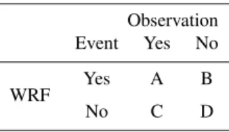
Scores are commonly used for validation purposes to statis-tically assess the performance of a model simulation relative to observations (validation) or to results of other model sim-ulation (inter-comparison). Some of them are derived from a 2×2 matrix called “contingency table” (e.g., Wilks, 1995), where each of the elements (A, B, C, D) holds the num-ber of combinations of model prediction and observation in a given statistical population (see Table 2). In this study, five different scores are used.

The bias score (BIAS) is defined as: BIAS=F

O=

A+B

A+C (1)

whereF is the number of cases where the event was pre-dicted, andO is the number of cases where the event was

Table 2. Contingency table used in the validation and sensitivity studies.

Observation Event Yes No

WRF Yes A B

No C D

observed. This score is an indicator of how well the model recovers the number of occurrences of an event, regardless of the spatio-temporal distribution.

The False Alarm Rate (FAR) computes the fraction of pre-dicted events that where not observed:

FAR=B

F =

B

A+B (2)

The Probability Of False Detection (POFD) is the fraction of predicted events that have not been observed relative to the total number of unobserved events:

POFD= B NO=

B

B+D (3)

Like the FAR the POFD is not a perfect indicator for valida-tion since it depends on the number of unobserved events, but is convenient for inter-comparison since it does not depend on the number of unpredicted events.

Similarly to the POFD the Probability Of Detection (POD) is the fraction of predicted events relative to the number of observed events:

POD= A

YES=

A

A+C (4)

Finally, the frequently used Heidke Skill Score (HSS) is de-fined:

HSS= S−SRef SPerf−SRef

(8)

whereS is the simulation score,SRef the probability of

de-tection by chance andSPerfthe score obtained by a perfect

simulation:

S=H

N =

A+D

N (6)

SRef=

(A+B)(A+C)+(B+D)(C+D)

N2 (7)

SPerf=1 (8)

His the number of hits, i.e., the number of cases where pre-diction and observation are in accordance, whileNis the size of the statistical population. The HSS indicates the capability of a simulation to be better or worse than a random simula-tion, and ranges from−1 to 1 (1 for a perfect and 0 for a random case).

In addition to the scores based on the contingency table, the standard Mean Bias (MB) and the Root Mean Square De-viation (RMSD) are defined as:

MB= 1 N

N X

i−1

(Pp−Po)i (9)

RMSD=

v u u t

1

N N X

i−1

(Pp−Po)2_i (10)

wherePpandPoare the predicted and observed precipitation

values.

3 Results

3.1 Validation of the control experiment

3.1.1 Validation of predicted precipitation by TRMM observations

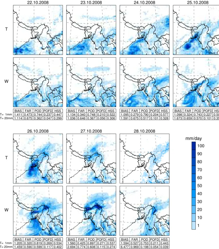
WRF30 and TRMM daily precipitation fields during the cy-clone life are presented for a subset of the LD in Fig. 4. The cyclonal precipitation patterns can be recognised in both data sets. The cyclone is traceable by the high daily precipitation following its movement. In the WRF30 output the centre of the cyclone shows a local precipitation minimum on 24 Octo-ber indicating that an eye has formed, which is, however, not present in the TRMM observations. On 25 October, the max-imum of daily precipitation amount observed by TRMM is following the centre of the cyclone. The eye is no longer vis-ible in the WRF30 output of this day. Both data sets accord-ingly show that strong precipitation caused by the cyclone occurs in the eastern and southern parts of Bangladesh. On 26 October the cyclone reaches the coast in the late evening hours. The precipitation maximum of this day is still over-seas for TRMM, whereas the WRF30 already predicts maxi-mum precipitation over Bangladesh. This discrepancy is ex-plainable by the difficulties in allocating the strong precipi-tation to the correct day. TRMM observes less precipiprecipi-tation

over Bangladesh on 27 October than the WRF30 predicts for that day. Over the Himalayas and the TiP, precipitation pat-terns are generally comparable. Two precipitation maxima are seen in both data sets, which were induced by the block-ing effect of the Himalayas over the slopes of Bhutan and by the eastern Nyainqentanglha Mountains. Also, both data sets show the precipitation front propagating over the TiP in a similar way.

Generally, WRF30 daily precipitation is larger than ob-served by TRMM, as indicated by the BIAS and FAR scores in Fig. 4. The two different threshold values used for com-putation of the scores in Fig. 4 show that a higher thresh-old lowers both the POD and the POFD. The HSS indicates that predictions based on small threshold values are generally better in accordance with TRMM than those based on high threshold values.

The spatial patterns presented in Fig. 5 reveal that WRF30–MD generally predicts more events, especially on the northern part of the TiP. Nevertheless, weather-stations measurements suggest that this northern limit is properly predicted. The two data sets are still in good agreement at 20 mm week−1_{, but the HSS constantly decreases as the FAR}

increases.

Both TRMM and WRF30–MD show precipitation max-ima of more than 60 mm week−1 _{in the eastern}

Nyainqen-tanglha Mountains and in north-eastern India, but more than 70 % of the 60 mm week−1_{events predicted by WRF30–MD}

were not observed by TRMM. However, the maximum in weather-station measurements on the eastern Nyainqentan-glha Mountains (138 mm week−1_{) suggests that the actual}

precipitation pattern may extend further in the western TiP than observed by TRMM. The reason behind this finding is probably the insufficient capability of the TRMM to detect snowfall and light rain.

WRF30-MD RMSD (54.3 mm week−1₎ _and _MB

(24.3 mm week−1_{) with respect to TRMM indicate}

gen-erally higher values predicted by WRF30 than observed by TRMM. The one-week HSS are higher than the daily scores presented in Fig. 4, most probably due to two major reasons: (1) possible discrepancies due to timing shifts are withdrawn when looking at the one-week precipitation amounts, (2) the considered spatial subset is different with respect to precipitation patterns.

3.1.2 Validation of predicted snow depth by MODIS observations

The goal of this test is to analyse where snowfall has been simulated by the WRF model in comparison to observational data.

(9)

BIAS FAR POD POFD HSS 1.411 0.473 0.744 0.237 0.447 1.114 0.675 0.362 0.047 0.299

22.10.2008

T

W

T= 1mm T= 20mm

23.10.2008

24.10.2008

25.10.2008

26.10.2008

T

W

T= 1mm T= 20mm

27.10.2008

28.10.2008

1 10 20 30 40 50 60 70 80 90 100 mm/day

Fig. 4.Daily precipitation fields (mm/day) from(T)TRMM and(W)WRF30 over a subset of the LD for the period 22 to 28 October 2008.

from the test, although snowfall might also have been occur-ring there. Unfortunately, large areas have been covered by clouds either in one or both of the two MODIS data sets, and thus have also to be marked as areas of no data.

We concentrated the validation on snow depth derived by the model from predicted snowfall. A grid point is

consid-ered to be covconsid-ered by snow when the computed snow depth after one-week exceeds a certain threshold. Spatial distribu-tions of predicted snow extent were computed for threshold values between 0.2 and 20 cm week−1_{. Five grid points at}

(10)

6 36 12

138 6

25

6

22

46

65

25 11

30

0

2 5

26 17

15

T= 10 mm/week

BIAS FAR POD POFD HSS 1.157 0.157 0.976 0.190 0.789

6 36 12

138 6

25

6

22

46

65

25 11

30

0

2 5

26 17

15

T= 20 mm/week

6 36 12

138 6

25

6

22

46

65

25 11

30

0

2 5

26 17

15

T= 60 mm/week

0 20 40 60 80 100

Threshold (mm/week) 0.0

0.2 0.4 0.6 0.8 1.0

Score

HSS

HSS FARFAR PODPOD POFDPOFD

WRF

TRMM

C

no D B

no

A

yes yes

Fig. 5. Left: Spatial patterns of the contingency tables for three different thresholds (10, 20 and 60 mm week−1_{) applied to the one-week} precipitation of WRF30–MD and TRMM, together with values from ground observations at the weather stations. Right: WRF30–MD scores with respect to TRMM for the threshold range from 1 to 100 mm week−1.

0 5 10 15 20

Snow depth threshold (cm) 0.0

0.2 0.4 0.6 0.8

HSS

0 5 10 15 20

0.2 0.4 0.6 0.8

HSS

WRF30−MD WRF10−MD

WRF30−SD WRF10−SD WRF2−SD

WRF

MODIS

C

no D

B no

A yes

yes

No data

WRF10−MD, T = 7.2 cm

Baingoin

Lhasa

Nagqu

Namco

WRF10−SD, T = 2 cm

Baingoin

Lhasa

Nagqu

Namco

WRF30−SD, T = 2 cm

Baingoin

Lhasa

Nagqu

Namco

WRF2−SD, T = 2 cm

(11)

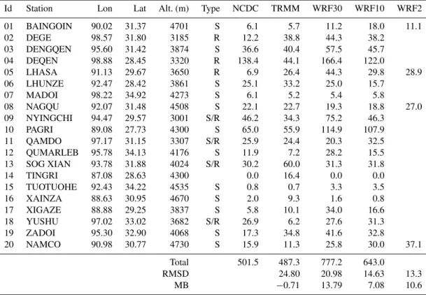
Table 3.Observed precipitation ( mm week−1_{) at each weather station (19 NCDC stations and the Nam Co weather station) in comparison} to the TRMM, WRF30, WRF10 and WRF2 results. The observed type of precipitation is indicated by R (rain) or S (snow). Root Mean Square Deviation (RMSD) and Mean Bias (MB) are indicated for each grid with respect to the NCDC data.

Id Station Lon Lat Alt. (m) Type NCDC TRMM WRF30 WRF10 WRF2

01 BAINGOIN 90.02 31.37 4701 S 6.1 5.7 11.2 18.0 11.1

02 DEGE 98.57 31.80 3185 R 12.2 38.8 44.3 38.2

03 DENGQEN 95.60 31.42 3874 S 36.6 40.4 57.5 45.7

04 DEQEN 98.88 28.45 3320 R 138.4 44.1 166.4 122.0

05 LHASA 91.13 29.67 3650 R 6.9 26.4 44.3 29.8 28.9

06 LHUNZE 92.47 28.42 3861 S 25.1 33.2 25.0 15.7

07 MADOI 98.22 34.92 4273 S 6.1 5.2 5.4 5.8

08 NAGQU 92.07 31.48 4508 S 22.1 22.7 19.3 18.8 27.0

09 NYINGCHI 94.47 29.57 3001 S/R 46.2 34.3 75.2 46.3

10 PAGRI 89.08 27.73 4300 S 65.0 55.9 114.9 107.9

11 QAMDO 97.17 31.15 3307 S/R 25.9 24.4 20.3 32.5

12 QUMARLEB 95.78 34.13 4176 S 11.9 7.2 28.2 15.5

13 SOG XIAN 93.78 31.88 4024 S/R 30.2 60.0 31.3 31.8

14 TINGRI 87.08 28.63 4300 0.0 16.4 0.0 0.0

15 TUOTUOHE 92.43 34.22 4535 S 0.8 0.7 3.3 3.5

16 XAINZA 88.63 30.95 4670 S 2.0 9.3 1.6 0.8

17 XIGAZE 88.88 29.25 3837 S 5.8 10.1 34.0 16.6

18 YUSHU 97.02 33.02 3682 S/R 26.9 6.2 27.6 31.3

19 ZADOI 95.30 32.90 4068 S 17.3 34.8 41.6 32.8

20 NAMCO 90.98 30.77 4730 S 15.9 11.3 25.8 30.0 37.1

Total 501.5 487.3 777.2 643.0

RMSD 24.80 20.98 14.63 13.3

MB −0.71 13.79 7.08 10.6

grids for the test (see Sect. 2.3). The area available for the test is finally reduced to 47.8 % in the MD and to 45.3 % in the SD. Snowfall was detected by MODIS on 21.6 % of the test area for the MD and on 83.9 % of the test area for the SD.

Wang et al. (2008) evaluated MODIS snow extent in north-ern Xinjiang, China, and they found that MODIS has high accuracies (93 %) when mapping snow at snow depth≥4 cm but does not have a proper accuracy for thinner layers. This threshold can be considered as physically reasonable: at the station Baingoin (north-west of Nam Co), 6 mm precipitation was recorded (6 cm of snow assuming a standard snow-to-liquid-equivalent ratio of 10), and the pixel was classified as snow by MODIS.

The evolution of the HSS with the threshold applied to the WRF simulated snow depth with respect to MODIS is shown in Fig. 6 (left) along with the spatial patterns of the contin-gency tables for two optimal thresholds for WRF10-MD and WRF-SD in the three resolutions. The HSS curves for the MD simulations are very similar, especially for lower thresh-olds, while there are more differences between the HSS curves for the SD. This is interpreted as an effect stemming from the higher spatial variability of snowfall in the MD due to large altitudinal variations compared to the less

hetero-geneous situation in the SD. In the Himalayas, the snow to rain limit is caught accurately by both WRF10 and WRF30 (not shown). Higher HSS for the simulations for model grids of higher spatial resolution, especially for higher thresholds, indicate the advantage of improved spatial resolution for pre-dicting snowfall, particularly in the SD. The maximum HSS for the SD is reached at a smaller threshold than for the MD. This difference is attributed to the fact that altitudes in the SD are generally higher than in the MD, thus the percent-age of areas affected by snowfall is higher as observed by MODIS due to generally lower air temperatures. Snow melt is less frequently occurring in the SD than in the MD, and therefore even small amounts of snowfall will increase the snow extent. This argument is also supported by the contin-gency maps displayed in Fig. 6, which reveal that most of the WRF2-SD snow extent not observed by MODIS is located in the lower-altitude valleys south of the western Nyainqentan-glha Mountains.

(12)

Table 4.Design of the sensitivity experiments.

Name Experiment New parameterisation

Nesting strategy

TW Nesting Two-way nesting (all domains) OW Nesting One-way nesting (all domains)

Forcing strategy

WI Initialisation Single initialisation and one-week continuous autonomous run WIN Forcing Single initialisation and

one-week continuous run with analysis nudging

Physical parameterisation schemes

CU1 Cumulus Betts-Miller-Janjic (BMJ) (Betts and Miller, 1986; Janjic, 1994) CU2 Cumulus Kain-Fritsch

(Kain and Fritsch, 1990) MP1 Microphysics WRF Single-Moment

6-class (WSM6)

MP2 Microphysics Goddard Cumulus Ensemble (GCE) (Tao et al., 2003) LS1 Land surface Rapid Update Cycle (RUC)

(Smirnova et al., 2000)

LS2 Land surface Pleim-Xiu (Pleim and Xiu, 1995) PBL1 PBL Yonsei University (YSU)

(Hong et al., 2006)

PBL2 PBL Asymmetrical Convective Model 2 (ACM2) (Pleim, 2007)

snow-free areas is situated in the north-western part of the SD, and is well detected by the WRF2-SD for the threshold of 2 cm. Increasing the threshold shifts the transitional zone to the South-west in all WRF simulations for the MD and SD, such that the contingency maps show a switch from false alarms to unpredicted events for all areas where prediction and observation are not concordant.

3.1.3 Validation of predicted precipitation by observations at weather stations

Table 3 shows observed precipitation at each weather station in comparison to precipitation observed by TRMM and pre-dicted by WRF30, WRF10 and WRF2. Results from the grid points nearest to the weather stations are used in the compar-ison.

Differences between the WRF simulations are generally small except for two stations: Nyingchi and Deqen, the later showing a large improvement from WRF30 to WRF10, il-lustrating the strong terrain dependency of precipitation in mountainous terrain. The RMSD and MB scores show a sig-nificant improvement from WRF30 to WRF10. Some dis-crepancies between station observations and TRMM could

0 5 10 15 20

0.1 0.2 0.3 0.4 0.5

HSS

0 5 10 15 20

0.1 0.2 0.3 0.4 0.5

HSS

WRF30−TW

WRF10−TW WRF2−TW (RE)

WRF30−OW (RE)

WRF10−OW WRF2−OW

WRF10−RE

Fig. 7. Sensitivity to the nesting strategy: HSS curves for snow depth predicted by WRF simulations (TW, OW and RE) at all reso-lutions for thresholds between 0.2 and 20 cm, with respect to snow extent observed by MODIS on the SD.

be explained by errors in one or the other data-set (at Lhasa, TRMM and WRF are in good agreement and at Deqen, sta-tion observasta-tions and WRF are concordant) and for some stations the three data-sets differ substantially. Generally, WRF10 has a lower RMSD than TRMM, but a higher MB.

Unfortunately, no in-depth evaluation for WRF2 could be made, because only four stations are situated in the SD. The results for these stations suggest a small but overall improve-ment to WRF10, again indicating the advantage of using model grids of higher spatial resolution.

3.2 Sensitivity study

In this section, we investigate the sensitivity of the WRF model to the nesting strategy, the forcing strategy, and var-ious physical parameterisations schemes (PPS). Table 4 pro-vides an overview on the sensitivity experiments carried out in this study, while Tables 5 and 6 present the results. 3.2.1 Sensitivity to the nesting strategy

(13)

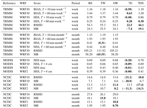
Table 5. Scores used for statistical evaluation of the reference, nesting and forcing experiments. The scores that differ of more than 10 % from the RE are marked in bold, and put between parentheses if they have a lower skill than the RE.

Reference WRF Score Period RE TW OW 7D 7DN

TRMM WRF30 BIAS,T= 10 mm week−1 week 1.16 1.18 1.16 (0.58) 1.10

TRMM WRF30 BIAS,T= 60 mm week−1 week 3.44 3.37 3.44 0.63 3.20

TRMM WRF30 HSS,T= 10 mm week−1 week 0.79 0.79 0.79 (0.48) 0.86

TRMM WRF30 HSS,T= 60 mm week−1 week 0.25 0.24 0.25 0.28 0.30

TRMM WRF30 RMSD week 54.3 55.3 54.3 22.5 44.1

TRMM WRF30 MB week 24.3 25.5 24.3 −7.4 19.1

TRMM WRF30 BIAS,T= 10 mm month−1 month 1.15 1.19 1.15

TRMM WRF30 BIAS,T= 60 mm month−1 month 1.93 1.93 1.93

TRMM WRF30 HSS,T= 10 mm month−1 month 0.41 (0.31) 0.41

TRMM WRF30 HSS,T= 60 mm month−1 month 0.44 0.48 0.44

TRMM WRF30 RMSD month 105.21 111.92 105.21

TRMM WRF30 MB month 58.20 (65.55) 58.20

MODIS WRF10 HSS max week 0.69 0.69 0.68 (0.20) 0.70

MODIS WRF10 HSS,T= 4 cm week 0.65 0.66 0.65 (0.09) 0.69

MODIS WRF2 HSS max week 0.43 0.43 0.40 (0.01) 0.43

MODIS WRF2 HSS,T= 4 cm week 0.39 0.39 0.36 (0.00) 0.41

NCDC WRF10 RMSD week 14.6 14.0 13.6 (31.2) 10.8

NCDC WRF10 MB week 7.1 7.1 6.6 (−20.0) 6.7

NCDC WRF2 RMSD week 13.3 13.3 11.4 13.3 (17.4)

NCDC WRF2 MB week 10.7 10.7 8.2 (−11.3) (14.3)

NCDC WRF10 RMSD month 27.8 26.1 29.0

NCDC WRF10 MB month 18.1 15.8 19.1

NCDC WRF2 RMSD month 13.1 13.1 10.8

NCDC WRF2 MB month 1.95 1.95 0.70

The results of all validation analyses applied to the TW and OW sensitivity experiments are presented in Table 5 to-gether with those of the reference experiment. Generally, the differences in the overall scores between the sensitivity experiments are small, indicating that this element of the experimental design is not highly sensitive for reanalysed precipitation fields.

The most suitable analysis for assessing the performance of the nesting experiments is presented in Fig. 7, where de-tection of snowfall in the SD is validated by the MODIS data on snow extent. Only in the SD the three different spa-tial resolutions can be compared to each other. A threshold value of 4 cm is used for comparing predicted snow depth with MODIS observations since this value is considered to be physically reasonable regarding the capability of MODIS for detecting snow (see Sect. 3.1.2). HSS curves of the TW experiments for detecting snowfall in the SD are generally higher than those of the respective OW experiments. Fig-ure 7 shows two major featFig-ures of the two-way nested ap-proach: the skill of the coarser resolutions is improved, and the higher-resolution results are also slightly meliorated by the step-wise feedback mechanism. Thus, the use of the two-way nesting option is recommended, although not being decisive for the overall performance.

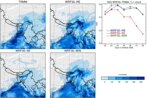
3.2.2 Sensitivity to the forcing strategy

Two experiments were carried out to analyse this element of the experimental design. In contrast to the other experiments, only the one-week period of the precipitation experiment was covered by the simulations. In contrast to the reference ex-periment, the model runs were only initialised once (incl. the 12 h spin-up). The weekly initialisation (WI) experiment is only forced at the lateral boundaries during integration time, while in the second experiment (WIN) weekly initialisation is combined with the analysis nudging option of the WRF, i.e., the WRF30-LD simulation is nudged towards GFS in-put data both horizontally and vertically using a point-by-point relaxation term for temperature, pressure and specific humidity.

(14)

TRMM WRF30−RE HSS WRF30−TRMM, T=1 mm/d

22 23 24 25 26 27 28

Days in October 2008 0.0

0.2 0.4 0.6

HSS

WRF30−RE WRF30−WI WRF30−WIN

WRF30−WI WRF30−WIN

5 40 80 120 160 200

mm/week

Fig. 8.Sensitivity to the forcing strategy. Left: one-week precipitation ( mm week−1_{) for TRMM, WRF30–RE, WRF30–WI and WRF30–} WIN over a subset of the LD. Right: daily HSS curves from WRF30 with respect to TRMM for the 1 mm day−1precipitation threshold over the same subset.

Table 6.Scores used for statistical evaluation of the reference and the eight PPS experiments. The scores that differ of more than 10 % from the RE are marked in bold, and put between parentheses if they have a lower skill than the RE.

Reference WRF Score Period RE CU1 CU2 MP1 MP2 LS1 LS2 PBL1 PBL2

TRMM WRF30 BIAS,T= 10 mm week 1.16 1.12 1.12 1.14 1.14 1.19 1.18 1.13 1.10

TRMM WRF30 BIAS,T= 60 mm week 3.44 (3.88) 3.76 3.38 3.77 3.55 3.45 3.51 3.78

TRMM WRF30 HSS,T= 10 mm week 0.79 0.82 0.80 0.80 0.81 0.76 0.77 0.81 0.82

TRMM WRF30 HSS,T= 60 mm week 0.25 0.29 0.30 0.26 0.24 0.25 0.24 0.26 0.26

TRMM WRF30 RMSD week 54.3 (76.5) (68.7) 55.4 56.1 54.3 55.4 53.5 (67.9)

TRMM WRF30 MB week 24.3 (35.8) (32.0) 24.4 26.7 25.6 25.4 23.8 (31.3)

TRMM WRF30 BIAS,T= 10 mm month 1.15 1.19 1.18 1.17 1.19 1.26 1.14 1.10 1.09

TRMM WRF30 BIAS,T= 60 mm month 1.93 1.81 1.92 1.90 1.98 (2.19) 1.93 1.78 1.77

TRMM WRF30 HSS,T= 10 mm month 0.41 (0.30) (0.35) (0.35) (0.33) (0.12) 0.44 0.52 0.54

TRMM WRF30 HSS,T= 60 mm month 0.44 0.49 0.45 0.45 0.44 (0.36) 0.45 0.49 0.49

TRMM WRF30 RMSD month 105.21 112.31 105.53 106.82 106.89 107.49 112.80 95.70 102.34

TRMM WRF30 MB month 58.20 61.73 60.03 58.86 58.47 (67.48) 62.76 50.30 52.97

MODIS WRF10 HSS max week 0.69 0.69 0.68 0.68 0.68 0.70 0.69 0.69

MODIS WRF10 HSS,T= 4 cm week 0.65 0.65 0.66 0.63 0.64 0.70 0.67 0.66

MODIS WRF2 HSS max week 0.43 0.41 0.40 0.40 0.40 0.45 0.42 (0.33)

MODIS WRF2 HSS,T= 4 cm week 0.39 (0.33) (0.29) (0.34) 0.36 0.40 (0.35) (0.22)

NCDC WRF10 RMSD week 14.6 13.7 11.9 15.8 (19.1) 14.2 14.2 11.7 11.1

NCDC WRF10 MB week 7.1 5.2 6.7 1.9 (13.7) (8.7) 7.5 7.1 6.7

NCDC WRF2 RMSD week 13.3 9.7 (16.8) 12.0 (17.7) 12.7 14.0 11.5 (17.0)

NCDC WRF2 MB week 10.7 7.0 10.3 8.0 (13.9) 10.7 10.1 8.9 11.6

NCDC WRF10 RMSD month 27.8 24.5 24.2 25.9 29.1 (34.1) 27.4 22.4 24.7

NCDC WRF10 MB month 18.1 13.3 18.5 12.4 (22.1) (27.4) 17.8 14.7 17.1

NCDC WRF2 RMSD month 13.1 15.7 (17.8) 12.5 (15.3) 12.3 13.6 10.4 (17.2)

(15)

accurate predictions when the large-scale forcing is missing, thus WI without analysis nudging is not a suitable forcing strategy.

In contrast, the WIN experiment performs as good as the reference experiment as the scores in Table 5 and the results displayed in Fig. 8 indicate. Although there are some minor deficiencies at 2 km spatial resolution, these are compensated by some minor advantages at the lower resolution of 30 km (and partly also of 10 km).

The applicability of the WIN forcing strategy is thus de-pending on the specific purpose followed by a model exper-iment. If precipitation fields of high spatial resolution are a major objective then daily re-initialisation remains the bet-ter choice. Also, the flexibility of the daily re-initialisation with respect to parallelisation of model runs is better than in the WIN strategy. In the RE design, daily model runs are completely independent from each other, and there are only minor jumps between the results of two consecutive days, which may be more problematic in the WIN strategy (al-though this aspect was not analysed in this study). A further argument for the forcing strategy followed in the RE design is the fact that the WRF model is able to better utilise its pre-dictive skills within the resolved scales, while analysis nudg-ing strongly dampens the mesoscale processes resolved by the WRF model.

3.2.3 Sensitivity to the PPS

In this part of the sensitivity study eight experiments were carried out, applying two different schemes for any of the CU, MP, LS and PBL parameterisation schemes (Table 4).

The results of all validation analyses applied to the PPS sensitivity experiments are presented in Table 6 together with those of the reference experiment. While a comparison of the scores mainly serves to show the effects of the different PPS and to assess the overall performance, the spatial distribu-tions of the differences between the PPS experiments and the reference experiment displayed in Fig. 9 provide insight into the mechanisms responsible for the differences.

Comparing the CU1 and CU2 experiments, the latter one has a lower performance, not only with respect to the CU1 experiment but also to the RE. The CU1 experiment im-proves the predictions with respect to the observations at weather stations while concurrently decreasing the predic-tions with respect to the TRMM observapredic-tions. Figure 9 shows that the sensitivity to the CU1 and CU2 experiments is very strong in the Bay of Bengal and the high-mountain fringes of the TiP, but is low on the TiP. Generally, the CU1 and CU2 experiments are wetter than the RE, especially in these regions. The reason for this finding is the convec-tive nature of precipitation in the sensiconvec-tive regions (as will be discussed in Sect. 4), while advection dominates large parts of the TiP. The three schemes work within different closure frameworks: for example, the PPS of the RE is a cloud ensemble scheme that uses 16 ensemble members to

obtain an ensemble-mean realisation at a given time and lo-cation, while the other two schemes are triggered on vari-ous conditions on the vertical uplift within an atmospheric column. Our results are in accordance with Mukhopadhyay et al. (2009) who compared convective parameterisations for RCM simulations during the monsoon season, and found that the PPS used in the CU1 and CU2 experiments underesti-mate the observations for lighter rain rates, and overestiunderesti-mate for higher rain rates, while the PPS used in the RE shows an overestimation for lighter rain rates. The predictive skill of the CU1 and CU2 PPS in the LD with respect to TRMM observations is lower than that of the RE (not shown in Ta-ble 6), thus the New Grell-Devenyi 3 scheme used in the RE could be recommended.

The scores of the MP1 and MP2 experiments presented in Table 6 reveal that the PPS of the MP2 experiment is not suitable for the TiP. The MP1 results show similar effects in Fig. 9 as discussed for the CU1 experiment: high sensitivity of this PPS in the regions of convective precipitation and low sensitivity on most parts of the TiP where advection dom-inates. We argue that the choices of the CU and MP PPS should also consider combinatory effects, but are less influ-ential for simulations in regions where advection is prevail-ing. These findings are interesting since the MP schemes are rather new and thus not extensively discussed in the scientific literature, so far.

The two experiments regarding the LS model underlying the WRF simulations show less pronounced effects when compared with the CU and MP PPS. The scores of the LS1 experiment reveal that larger differences to the RE are neg-ative, thus this PPS would have to be rejected from these findings. However, there are also minor improvements in the simulation of snow processes, which may give reason for us-ing this PPS when snow-hydrological investigations are in the focus of a model study. The LS2 experiment, in con-trast, shows that no stronger negative effects are arising from this PPS, but unfortunately, it does not include an explicit parameterisation of snow processes, and thus makes it in-appropriate for snow-hydrological investigations. Figure 9 shows that the effects of the two LS models are weak not only on the TiP but also in the regions where the CU and MP PPS show strong sensitivities. This can be attributed to the fact that convective processes and related MP processes are only weakly influenced by the underlying land surface, but mainly depend on the atmospheric dynamics and physics themselves. Over longer time periods, the choice of the LS model is expected to become more influential, but this aspect was not investigated in our study.

(16)

CU1 CU2 MP1

MP2 LS1 LS2

PBL1 PBL2

−75 −50 −25 0 25 50 75 mm/week

Fig. 9.Sensitivity to the physical parameterisation schemes. Difference between the one-week precipitation ( mm week−1_{) of the sensitivity} experiments and the RE for WRF30 over a subset of the LD.

NWP models to the PBL parameterisation is also in this case stronger than to microphysics, at least for the regions south from the TiP. Figure 9 shows an interesting effect: the spatial pattern of the differences between the PBL2 experiment and the RE are strongly coupled to both CU PPS, since it also considers convective processes in the PBL.

In conclusion of the sensitivity studies for the PPS, we could show that there is nothing like a perfect combination of PPS, since any model-based investigation of precipitation on the TiP has to consider the oceanic regions where much of the water vapour and the convective systems influencing the southern, central and eastern parts of the TiP are formed. Yang and Tung (2003) also concluded that it was not pos-sible to define a best performing cumulus parameterisation since each of the investigated cumulus schemes performed very differently for precipitation prediction under different

synoptic forcing. Depending on the focus of an investigation, slightly modified PPS combinations may be used, but gener-ally, the PPS combination used in the RE seems suitable for reanalysing precipitation on the TiP.

4 Discussion

(17)

4.1 Validation methods and data sets

In this study, we proposed three data sets (TRMM, MODIS, NCDC weather stations) and several statistical methods to assess the WRF model simulations. Several climatological studies used the TRMM products, and it has been proven that TRMM 3B42 surface-rainfall rate is comparable to other surface observations (Koo et al., 2009), although the spatial scale of the rainfall data makes direct comparison to gauge data difficult. Our results also enlighten this issue: the WRF model and precipitation data sets depicted some consider-able discrepancies when compared to point-by-point mea-surements at weather stations. TRMM showed to be less ef-ficient than WRF10. Estimation errors due to spatial resolu-tion may be reduced by statistical correcresolu-tion methods as de-scribed by Yin et al. (2008), but the authors also remind that TRMM performs poorly during the winter months, because of the presence of snow and ice over the TiP, since snow and ice on the ground scatter microwave energy in a similar fash-ion as ice crystals and raindrops in the atmosphere.

At the same time, TRMM offers a way to assess the mesoscale WRF30 output on a gridded spatial basis, and the two data sets are in good accordance for the spatial delin-eation of the 10 mm week−1_{precipitation event. The}

com-parison also showed differences in the occurrence of ex-treme events, for which WRF30 predicts higher amounts than TRMM observes. India’s weather stations in the north-eastern provinces recorded precipitation amounts up to 150 mm day−1 _{during the event (IMD, 2008), which is}

lower than the highest values predicted by WRF (up to 500 mm week−1_{for a few points at the high-mountain fringe}

of the TiP) but higher than TRMM estimations (maximum values of 130 mm week−1_).

One of the strengths of the WRF model is its ability to separate snow from rain. Since we are targeting on using the regional atmospheric reanalysis for hydrological and glacio-logical applications, snow data are of great importance, and the MODIS test that we developed proved to give valuable in-formation on the models capacity to retrieve snowfall at high spatial resolution, as e.g. indicated by the positive effect of increasing spatial resolution and the use of two-way nesting. However, snow extent could be detected only where no snow prior to the event or clouds was present, preventing us draw-ing conclusions on high-mountain snowfall. Furthermore, it is rather difficult to find a suitable event or to run this test on a regular and automatic basis.

So far, no robust assessment of the WRF2 output is possi-ble with weather stations either, as they are too scarce. More-over, rain gauges do have a high sensitivity to wind and to the size of snow/rain particles: the snow under-catch of the four most widely used gauges can vary up to 80 % (Goodi-son et al., 1998). On response to this problem, we installed a Laser precipitation monitor (Distrometer) at the Nam Co station for future validation studies.

We applied a combination of different validation methods since none of the observational data sets could be unambigu-ously identified to serve as an absolute reference for model validation. Despite the discussed differences between the model experiments and the observational data sets (including differences between the observational data sets themselves) the model predictions and the observational data are gener-ally concordant. Thus, we consider the validation methods and data sets principally suitable for this kind of studies. 4.2 Reanalysis of precipitation fields over the TiP

The WRF model offers a countless number of configurations, and in this study there was no intent to realise a complete re-view of the various possibilities. We assessed the sensitivity of the WRF model to different PPS. In general, the influ-ence on predicted precipitation was rather small on the TiP in comparison to the forcing strategies. This can be due to frequent re-initialisation constraining the model to stay close to the large scale observations given as input data.

The comparison with observational data sets showed that the WRF model had a good accuracy in predicting snow- and rainfall of a single precipitation event. Tables 5 and 6 also present the scores for the one-month simulations carried out for October 2008, which are showing that the WRF model is generally able not only reanalysing precipitation over longer time periods including also times of no precipitation.

Figure 10 presents two results illustrating both the reason for the applicability of our approach and the hydrological relevance of individual precipitation events. The upper two maps display the contribution of convective precipitation to the total precipitation for the one-week simulation period of the Rashmi event. Except for the central and north-western part of the TiP, advection prevails and enables to retrieve ac-curate precipitation values within the error limits of the ob-servations. In regions of high contribution of convective pre-cipitation the sensitivity of the two CU and MP PPS, as well as the PBL2 PPS are much higher than in the other regions, which explains why the PPS schemes are not as important on the TiP. The dominance of advection on the TiP also allows reanalysing precipitation fields at high spatial resolution of 2 km without using a CU parameterisation scheme that is re-quired at the lower resolutions of 10 and 30 km.

(18)

Convective precipitation − WRF30 Convective precipitation − WRF10

0 10 20 30 40 50 60 70 80 90 100 %

Event contribution to one−month prcp − WRF30 Event contribution to one−month prcp − WRF10

0 10 20 30 40 50 60 70 80 90 100 %

Fig. 10. Top: contribution of convective precipitation to the total precipitation for the one-week simulation period of the Rashmi event. Bottom: contribution of precipitation caused by the Rashmi event to monthly precipitation in October 2008.

Not only precipitation amounts but also the capture and timing of precipitation events is of high hydrological rele-vance. Figure 11 presents time-series of accumulated precip-itation amounts for October 2008 from NCDC, TRMM and WRF10 at the 19 weather stations to analyse the capability of the WRF model capturing precipitation events close to the time they are also observed. In addition, we indicate the ex-plained variance (r2) of the daily accumulated time-series for each pair of data sets.

At five weather stations monthly precipitation amounts predicted by WRF10 are close to ground observations, while TRMM observations are close to ground measurements at four weather stations. Similar values for monthly precipi-tation amounts are retrieved by WRF10 and TRMM at four weather stations, where ground observations strongly differ from these values. Ground observations are much higher than TRMM or WRF10 only at two weather stations, while much lower values are reported at six weather stations. These results are in general accordance with the findings that were previously discussed for the single event.

Generally, WRF10 is better in explaining the variance in the ground observations than TRMM. With the exception of three stations WRF10 is better correlated with ground obser-vations than TRMM. The generally very highr2 values of WRF10 with the two observational data sets indicate that the

WRF model is well-suited to retrieve precipitation dynamics, including times of no precipitation. This holds true even for many of the cases where the precipitation amounts for Oc-tober 2008 simulated by WRF10 differs from one or both of the observations.

Positive mean bias values also found in other model vali-dation studies are often interpreted as an error produced by the model. However, since the problems in observing pre-cipitation are well-documented, resulting in systematically lower values especially for snowfall, we argue that this bias also documents the observational errors. Our study could not prove systematic, statistically significant over-prediction of precipitation by WRF10, although there are certainly indi-vidual cases, where WRF10 values are actually too high.

(19)

BAINGOIN (90.0E, 31.4N)

5 10 15 20 25 30 0

10 20 30

Acc. prcp (mm)

BAINGOIN (90.0E, 31.4N)

5 10 15 20 25 30 0

10 20 30

Acc. prcp (mm)

r2

WRF,NCDC = 0.94

r2TRMM,NCDC = 0.94

r2

TRMM,WRF = 0.92

DEGE (98.6E, 31.8N)

5 10 15 20 25 30 0 20 40 60 80 100 120 r2

WRF,NCDC = 0.93

r2TRMM,NCDC = 0.51

r2

TRMM,WRF = 0.71

DENGQEN (95.6E, 31.4N)

5 10 15 20 25 30 0 20 40 60 80 r2

WRF,NCDC = 0.87

r2TRMM,NCDC = 0.78

r2

TRMM,WRF = 0.94

DEQEN (98.9E, 28.5N)

5 10 15 20 25 30 0

50 100 150

r2

WRF,NCDC = 0.98

r2TRMM,NCDC = 0.91

r2

TRMM,WRF = 0.89

LHASA (91.1E, 29.7N)

5 10 15 20 25 30 0

10 20 30 40

Acc. prcp (mm)

r2

WRF,NCDC = 0.87

r2TRMM,NCDC = 0.85

r2

TRMM,WRF = 0.97

LHUNZE (92.5E, 28.4N)

5 10 15 20 25 30 0 10 20 30 40 50 r2

WRF,NCDC = 0.77

r2TRMM,NCDC = 0.86

r2

TRMM,WRF = 0.78

MADOI (98.2E, 34.9N)

5 10 15 20 25 30 0 10 20 30 40 50 r2

WRF,NCDC = 0.87

r2TRMM,NCDC = 0.57

r2

TRMM,WRF = 0.71

NAGQU (92.1E, 31.5N)

5 10 15 20 25 30 0

20 40 60

r2

WRF,NCDC = 0.94

r2TRMM,NCDC = 0.87

r2

TRMM,WRF = 0.84

NYINGCHI (94.5E, 29.6N)

5 10 15 20 25 30 0

20 40 60 80

Acc. prcp (mm)

r2

WRF,NCDC = 0.92

r2_{TRMM,NCDC = 0.89}

r2

TRMM,WRF = 0.90

PAGRI (89.1E, 27.7N)

5 10 15 20 25 30 0 50 100 150 200 r2

WRF,NCDC = 0.92

r2

TRMM,WRF = 0.97

QAMDO (97.2E, 31.2N)

5 10 15 20 25 30 0 20 40 60 80 r2

WRF,NCDC = 0.91

r2

TRMM,WRF = 0.89

QUMARLEB (95.8E, 34.1N)

5 10 15 20 25 30 0

20 40 60

r2

WRF,NCDC = 0.92

r2

TRMM,WRF = 0.88

SOG_XIAN (93.8E, 31.9N)

5 10 15 20 25 30 0

20 40 60 80

Acc. prcp (mm)

r2

WRF,NCDC = 0.96

r2TRMM,WRF = 0.88

TINGRI (87.1E, 28.6N)

5 10 15 20 25 30 0

10 20 30

r2

WRF,NCDC = 0.26

r2TRMM,WRF = 0.42

TUOTUOHE (92.4E, 34.2N)

5 10 15 20 25 30 0 20 40 60 80 r2

WRF,NCDC = 0.91

r2TRMM,WRF = 0.80

XAINZA (88.6E, 31.0N)

5 10 15 20 25 30 0 5 10 15 20 r2

WRF,NCDC = 0.30

r2TRMM,WRF = 0.51

XIGAZE (88.9E, 29.3N)

5 10 15 20 25 30 Days

0 10 20 30

Acc. prcp (mm)

r2WRF,NCDC = 0.99

r2TRMM,WRF = 0.65

YUSHU (97.0E, 33.0N)

5 10 15 20 25 30 Days 0 20 40 60 80 100

r2WRF,NCDC = 0.96

r2TRMM,WRF = 0.78

ZADOI (95.3E, 32.9N)

5 10 15 20 25 30 Days 0 20 40 60 80 100

r2WRF,NCDC = 0.94

r2TRMM,WRF = 0.81

STATION

WRF

TRMM

r2

WRF,NCDC = 0.85

r2

TRMM,WRF = 0.80

Fig. 11.Time series of daily precipitation amounts accumulated during October 2008 observed at weather stations, by TRMM and predicted by the one-month WRF10 simulation. Explained variances (r2) are given for each pair of the three data sets and each station, as well as the meanr2for all stations. X-axis values are the days in October, the grey band marks the one-week focus period 22–28 October 2008.

resolution. Bookhagen and Strecker (2008) analysed oro-graphic precipitation along the eastern Andes, showing that only TRMM 2B31 data, which has a high spatial resolution of about 5 km is able to depict the small-scale orographic influence on precipitation. However, these data are not