Volume 2 PROGRESS IN PHYSICS April, 2008
On the Second-Order Splitting of the Local-Time Peak
Victor A. Panchelyugaand Simon E. Shnolly
Institute of Theor. and Experim. Biophysics, Russian Acad. of Sciences, Pushchino, Moscow Region, 142290, Russia yDepartment of Physics, Moscow State University, Moscow 119992, Russia
Corresponding authors. Victor A. Panchelyuga: [email protected]; Simon E. Shnoll: [email protected]
The paper presents experimental investigations of a local-time peak splitting right up to a second-order splitting. The splitting pattern found in the experiments has a fractal structure. A hypothesis about the possibility of high order splitting is proposed. The obtained experimental result leads to a supposition that the real space possesses a fractal structure.
1 Introduction
The main subject of this paper is a local-time effect, which is one of manifestations of the phenomenon of macroscopic fluctuations. The essence of this phenomenon is that the pat-tern (shape) of histograms, which are built on the base of short samples of the time series of the fluctuations measured in the processes of different nature, are non-random. Many-years of investigations of such histograms carried out by the method of macroscopic fluctuations [1] revealed a variety of phenom-ena [2–4]. The most important among the phenomphenom-ena is the local-time effect [5–8].
The local-time effect consists of the high probability of the similarity of the histogram pairs, which are divided by a time interval equal to the local-time difference between the points of measurement. This effect was registered in the scale of distances from the maximal distance between the loca-tions of measurement which are possble on the Earth’s sur-face (about 15,000 km) to the distances short as 1 meter. Be-sides, this effect can be observed on the processes of very different nature [2–4].
The idea of a typical local-time experiment is illustrated by Fig. 1. There in the picture we have two spaced sources of fluctuations 1 and 2, which are fixed on the distance L between them, and synchronously moved with a velocityV in such a way that the line which connects 1 and 2 is parallel to the vector of the measurement system’s velocityV. In this case, after a time durationt0
t0=VL; (1) the source of fluctuations 1 appear in the same position that the source 2 was before. In Fig. 1 these new places are pre-sented as 10 and 20. According to the local-time effect, co-incident spatial positions cause similar histograms patterns. In the interval distribution built on the base of the measure-ments carried out by the system displayed in Fig. 1 (the num-ber of similar pairs of the histograms as a function of the time interval between them), a single peak in the intervalt0 is observed.
In our previous works [6-8], we showed that there within
Fig. 1: This diagram illustrates the appearance of the local-time effect.
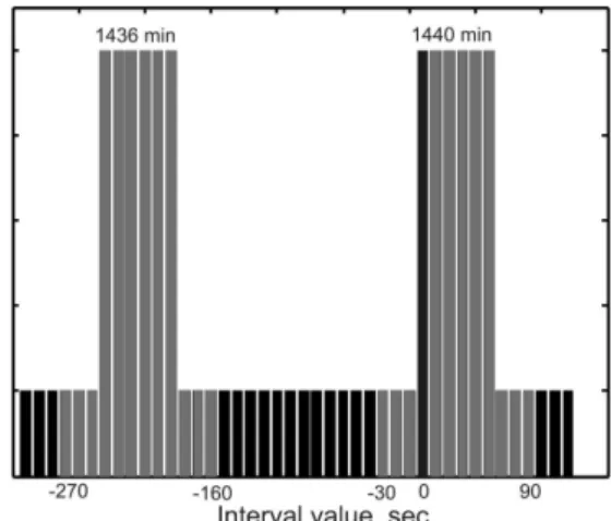
Fig. 2: The sketch of the solar (1440 min) and stellar (1446 min) splitting of the daily period.
the time resolution enhancement (with use histograms, short-est in time) the local-time peak splits onto two sub-peaks. It was found that the ratio between the splittingt1 and the local-time valuet0isk =2.7810 3. This numerical value is equal, with high accuracy, to the ratio between the daily pe-riod splitting 240 sec and the daily pepe-riod value T =86400 sec [7, 8]. This equality means that the local-time effect and the daily period are originated in the same phenomenon. From this viewpoint, the daily period can be considered as the maximum value of the local-time effect, which can be ob-served on the Earth.
In our recent work [8], we suggested that the sub-peaks of the local-time peak can also be split with resolution enhance-ment, and, in general, we can expect ann-order splitting with the valuetn
tn= knt0; n = 1; 2; 3; : : : (2)
April, 2008 PROGRESS IN PHYSICS Volume 2
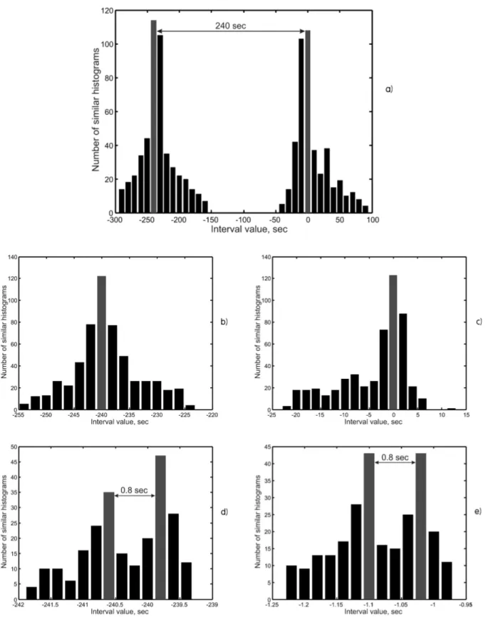
Fig. 3: The interval distributions for the 10-sec histograms (a), 2-sec histograms (b)–(c), and 0.2-sec histograms (d–e).
Volume 2 PROGRESS IN PHYSICS April, 2008
Preliminary results obtained in [8] verified this suggestion in part. The present work provides further investigation on the second-order splitting of the local-time peak.
As easy to see, from (2), every subsequent value of the local-time peak splittingtnneeds more than two orders of resolution enhancement. Therefore, most easy way to study
tnis to use the maximum value oft0. Such a value, as
stated above, is the daily periodt0=86400 sec.
2 Experimental results
To study the second-order splitting of the daily period, we use the known positions of the “solar peak” (1440 min) and the “sidereal peak” (1436 min), which are the first-order split-tings of the daily period. The peaks are schematically dis-played in Fig. 2. To find the position of the second-order split-ting peaks, we used the method of consecutive refinements of the positions of the solar and sidereal peaks. The peaks displayed in Fig. 2 are determined with one-minute accuracy. Since the positions of the solar and stellar peaks are well-known, we can study its closest neighborhood by shortest (to one minute) histograms. In Fig. 2, such a neighborhood is displayed by gray bars (they mean 10-sec histograms). After obtaining the intervals distribution for the 10-sec histograms, the procedure was repeated, while the rˆole of the 1-min his-tograms was played by the 10-sec hishis-tograms, and those were substituted for the 2-sec histograms. After this, the procedure was on the 2-sec and 0.2-sec histograms.
Zero interval (Fig. 2) marked by black colour corresponds to the start-point of the records. We used two records, started in the neighboring days at the same moments of the local time. So, the same numbers of histograms were divided by the time interval equal to the duration of solar day: 86400 sec. The interval values shown in Fig. 2 are given relative to zero interval minus 86400 sec.
The time series of the fluctuations in a semiconductor diode were registered on November 2–4, 2007. Each of the measurement consisted of two records with a length of 50000 and 19200000 points measured with the sampling rate 5 Hz and 8 kHz. On the base of these time series, we built the sets of the 10-sec, 2-sec, and 0.2-sec histograms. We used these sets in our further analysis.
The 10-second set of histograms was built on the base of the records, obtained with the sampling rate 5 Hz. Each 10-sec histogram was built from 50 points samples of the time series of fluctuation. The 2-sec and 0.2-sec sets were built on the base of the 50-point samples of the 25 Hz and 250 Hz time series (they were recount from the 8 kHz series).
It is important to note, that the solar day duration is not equal exactly to 86400 sec, but oscillates along the year. Such oscillations are described by the time equation [8]. To provide our measurements, we choose the dates when the time equa-tion has extrema. Due to this fact, the day duraequa-tion for all the measurements can be considered as the same, and we can
Fig. 4: The daily period splitting. Gray color marks the experimen-tally found splittings. The splitting displayed below were calculated on the base of the formula (2) forn =3. . . 5.
average the interval distributions obtained on the base of the time series measured on November 2–4, 2007.
The interval distributions obtained after the comparison of the histograms are given in Fig. 3. The upper graph, Fig. 3a, displays the interval distribution for the 10-sec histograms. As follows from Fig. 3a, the interval distribution in the neigh-borhood of the 1-min peaks consists of two sharp peaks (dis-played by gray bars) which are separated by a time interval of 24010 sec giving the positions of the solar and sidereal peaks with 10-sec accuracy.
The interval distributions in the neighborhood of the 10-sec peaks (Fig. 3a), for the 2-10-sec histograms, are displayed in Fig. 3b–3c. Gray bars in Fig. 3b–3c correspond to the new positions of the solar and sidereal peaks with 2-sec accuracy. Considering the neighboring of the 2-sec peaks (Fig. 3b–3c) to the 0.2-sec histograms, we obtain the interval distributions displayed in Fig. 3d–3e. As easy to see, instead of the more precise position of the 2-sec solar and sidereal peaks, we ob-tain the splitting of the aforementioned peaks onto two cou-plets of new distinct peaks. So, from Fig. 3d–3e, we state the second-order splitting of the daily period.
3 Discussion
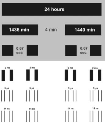
On the base of the formula (2), forn =2 with use oft0=
=86400 sec andk =2.7810 3 for the second-order split-ting t2, we get the valuet2=0.67 sec. From the
April, 2008 PROGRESS IN PHYSICS Volume 2
perimentally obtained interval distribution (Fig. 3d–3e), we havet2=0.80.2 sec. So, the experimental value agrees with the theoretical estimations made on the base of the for-mula (2).
Such an agreement leads us to a suppositon that there is a high-order splitting, which can be obtained from the for-mula (2). In Fig. 4, we marked by gray colour the experi-mentally found splitting. The splitting displayed below was calculated on the base of (2) forn =3. . . 5,t0=86400 sec, andk =2.7810 3. This splitting will be a subject of our further studies, and only this splitting is accessed to be stud-ies now. Forn >5, we will need to get measurements with a sampling rate of about 7.5 THz. Such a sampling rate is out of the technical possibilities for now.
As was stated in Introduction, the local-time effect exists in the scale from the maximal distances, which are possible on the Earth’s surface, to the distances close to one meter. Besides, the local-time effect doesn’t depend on the origin (nature) of the fluctuating process. In the case, where the spa-tial basis of the measurements is about one meter, the time required for obtaining of the long-length time series (that is sufficient for further analysis) is about 0.5 sec. Any exter-nal influences of geophysical origin, which affect the sources of the fluctuations synchronously, cannot be meant a source of the experimentally obtained results. Only the change we have is the changing of the spatial position due to the motion of whole system with a velocityV originated in the rotatory motion of the Earth (see formula 1). From this, we can con-clude that the local-time effect originates in the heterogeneity of the space itself. The results presented in Fig. 3 lead us to a supposition that such an heterogeneity has a fractal structure.
Submitted on February 11, 2008 Accepted on March 10, 2008
References
1. Shnoll S.E. and Panchelyuga V.A. Macroscopic fluctuations phenomena. Method of measurements and experimental data processing.World of measurements, 2007, no. 6, 49–55.
2. Shnoll S.E., Kolombet V.A., Pozharskii E.V., Zenchenko T.A., Zvereva I.M., and Konradov A.A. Realization of discrete states during fluctuations in macroscopic processes.Physics-Uspekhi, 1998, v. 41(10), 1025–1035.
3. Shnoll S.E., Zenchenko T.A., Zenchenko K.I., Pozharskii E.V., Kolombet V.A., and Konradov A.A. Regular variation of the fine structure of statistical distributions as a consequence of cosmophysical agents. Physics-Uspekhi, 2000, v. 43(2), 205–209.
4. Shnoll S.E. Periodical changes in the fine structure of statis-tic distributions in stochasstatis-tic processes as a result of arithmestatis-tic and cosmophysical reasons.Time, Chaos, and Math. Problems, no. 3, Moscow University Publ, Moscow, 2004, 121–154.
5. Panchelyuga V.A. and Shnoll S.E. On the dependence of a local-time effect on spatial direction.Progress in Physics, 2007, v. 3, 51–54.
6. Panchelyuga V.A. and Shnol’ S.E. Space-time structure and macroscopic fluctuations phenomena.Physical Interpretation of Relativity Theory. Proceedings of International Meeting, Moscow, 2–5 July 2007, Edited by M. C. Duffy, V. O. Gla-dyshev, A. N. Morozov, and P. Rowlands, Moscow, BMSTU, 2007, 231–243.
7. Panchelyuga V.A., Kolombet V.A., Panchelyuga M.S., and Shnoll S.E. Experimental investigations of the existence of local-time effect on the laboratory scale and the heterogeneity of space-time.Progress in Physics, 2007, v. 1, 64–69.
8. Mikhaylov A.A. The Earth and its rotation. Moscow, Nauka, 1984, 80 p.