TRANSPORT MODELLING: MACRO AND MICRO SIMULATION FOR THE STUDIED CASE OF FUNCHAL

TRANSPORT MODELLING: MACRO

AND MICRO SIMULATION FOR THE

STUDIED CASE OF FUNCHAL

A thesis submitted for the degree of Master of Civil Engineering at the Center of Exact

Sciences and Engineering of the University of Madeira

by

RITA RODRIGUES

Supervisor

Prof. Lino Maia

(University of Madeira - UMa)

Co-supervisors

Prof. Ángel Ibeas

(University of Cantabria - UC)

Dr. Claudio Mantero

(Horários do Funchal - HF) (Research and Planning Department)

Title: Transport Modelling: Macro and Micro Simulation for the studied case of Funchal

Keywords: Transport, model, macro simulation, micro simulation, mobility, environmental study. Author: RITA RODRIGUES

CCEE – Center of Exact Sciences and Engineering Department of Civil Engineering

UMa - University of Madeira Caminho da Penteada, s/n 9020 - 105 Funchal, Portugal Telephone + 351 291 705 230 E-mail: [email protected]

Jury:

Luigi Dell’Olio; University of Cantabria – UC

Lino Manuel Serra Maia; University of Madeira – UMa

João Paulo Martins; University of Madeira – UMa

José Manuel dos Santos; University of Madeira – UMa

A

The work done in this thesis attempts to demonstrate the importance of using models that can predict and represent the mobility of our society. To answer the proposed challenges two models were examined, the first corresponds to macro simulation with the intention of finding a solution to the frequency of the bus company Horários do Funchal, responsible for transport in the city of Funchal, and some surrounding areas. Where based on a simplified model of the city it was possible to increase the frequency of journeys getting an overall reduction in costs.

The second model concerns the micro simulation of Avenida do Mar, where currently is being built a new roundabout (Praça da Autonomia), which connects with this avenue. Therefore it was proposed to study the impact on local traffic, and the implementation of new traffic lights for this purpose. Four possible situations in which was seen the possibility of increasing the number of lanes on the roundabout or the insertion of a bus lane were created. The results showed that having a roundabout with three lanes running is the best option because the waiting queues are minimal, and at environmental level this model will project fewer pollutants.

R

O trabalho realizado nesta tese pretende sensibilizar para a importância do uso de modelos capazes de prever e de representar a mobilidade da nossa sociedade. Para responder aos desafios propostos, foram realizados dois modelos, um primeiro no âmbito da macro simulação com a intenção de encontrar uma solução para a frequência dos autocarros da companhia Horários do Funchal, responsável pelo transporte público na cidade do Funchal, e de algumas zonas envolventes a esta. Assim, com base num modelo simplificado da cidade foi possível aumentar a frequência das carreiras obtendo uma redução global de custos.

O segundo modelo diz respeito à micro simulação da Avenida do Mar – de momento está a ser construída uma nova rotunda (Praça da Autonomia), que faz ligação com esta avenida. Foi proposto estudar o impacto desta rotunda no trânsito local, e a implementação de novos semáforos para tal efeito. Foram criados quatro situações possíveis em que foi vista a possibilidade de aumentar o número de vias na rotunda ou a inserção de uma via de autocarro. Os resultados obtidos demonstraram que a melhor opção é a rotunda a funcionar com três vias, pois as filas de espera são mínimas. Para além disso, a nível ambiental este modelo apresenta menos projeções de gases poluentes.

T

C

Abstract ... v

Resumo ... vii

Table of Contents ... ix

List of Pictures ... xiii

List of Tables ... xv

Terminology ... xvii

Acknowledgments ... xix

1. INITIAL CONSIDERATIONS ... 1

1.1. Introduction ... 1

1.2. Motivations ... 2

1.3. Objectives ... 3

1.4. Framework ... 3

1.5. Limitations and scientific contribution ... 3

1.6. Presentation of the thesis ... 4

2. STATE-OF-THE-ART TRANSPORT PLANNING AND MODELLING ... 5

2.1. Background ... 5

2.2. Models and their role... 6

2.3. Characteristics of transport problems ... 7

2.4. Data and space ... 9

2.4.1. Methods to collect data ... 9

2.5. Trip generation and distribution models ... 11

2.5.1. Growth factor method ... 13

2.5.2. Gravity model ... 14

2.5.3. Intervening opportunities model ... 14

2.5.4. Choice model... 15

2.5.5. Entropy Model... 15

2.6. Modelling and decision making ... 16

3. MACROSCOPIC SIMULATION ... 19

3.1. Introduction ... 19

3.2.1. Trip generation ... 21

3.2.2. Trip distribution ... 21

3.2.3. Modal split ... 22

3.2.4. Traffic assignment ... 22

3.3. Network representation... 22

3.3.1. Study zone ... 23

3.3.2. Mobility in Funchal ... 24

3.3.3. System of collective transport ... 25

3.3.4. Hierarchy of roads ... 26

3.3.5. Survey and count post information ... 27

3.3.6. Traffic count ... 27

3.3.7. Speeds ... 28

3.3.8. Saturation ... 29

3.4. Performance Indicators ... 29

3.4.1. Average Waiting Time at Origin ... 30

3.4.2. Average Speed of Movement ... 30

3.4.3. Average Travel Speed ... 30

3.4.4. Average Number of Transshipments ... 30

3.4.5. Percentage of Direct Travel ... 31

3.5. Network calibration and validation ... 31

3.6. Bus Frequencies ... 32

3.6.1. Proposed optimization model ... 32

3.6.2. Projected solution ... 34

3.7. Results and Discussion ... 35

4. MICROSCOPIC SIMULATION ... 41

4.1. Introduction ... 41

4.2. Study Zone ... 42

4.3. Network representation... 43

4.3.1. Network layout ... 43

4.3.2. Traffic demand data ... 44

4.3.3. Traffic control ... 45

4.3.3.1. Furness distribution model ... 47

4.3.4. Public transport ... 50

4.3.5. Initial state ... 50

4.5. Scenarios ... 51

4.6. Results ... 54

4.6.1. Environmental study ... 56

4.7. Discussion of Results ... 60

5. FINAL CONSIDERATIONS ... 63

5.1. Conclusions and Final Remarks ... 63

5.2. Future Developments ... 65

REFERENCES ... 67

L

P

Figure 2.1 – Vicious circle of urban decline ... 7

Figure 2.2 – Breaking the car/public-transport vicious circle ... 8

Figure 2.3 – Trip types ... 12

Figure 2.4 – Rational planning ... 18

Figure 3.1 – The four-stage model in its basic form ... 20

Figure 3.2 – Funchal zone distribuition ... 24

Figure 3.3 - Classification of the road network by hierarchical level ... 26

Figure 3.4 – Data Post Locations ... 27

Figure 3.5 – Progress of traffic in the sum of all the counting stations. ... 28

Figure 3.6 – Average Velocities. ... 29

Figure 3.7 – VStromFuzzy method ... 31

Figure 4.1 – Avenida do Mar ... 42

Figure 4.2 – Traffic lights location. ... 45

Figure 4.3 – Traffic lights location in the roundabout. ... 47

Figure 4.4 – Flow on Praça de Autonomia ... 48

Figure 4.5 – Praça da Autonomia entries and exits designations ... 51

Figure 4.6 – Model of Case 1. ... 52

Figure 4.7 – Model of Case 2. ... 52

Figure 4.8 – Model of Case 3. ... 53

Figure 4.9 – Model of Case 4. ... 53

Figure 4.10 – Queue length formed by cars in the entry of roundabout to Case 1. ... 54

Figure 4.11 – Queue length formed by cars in the entry of roundabout to Case 2. ... 54

Figure 4.12 – Queue length formed by cars in the entry of roundabout to Case 3. ... 55

Figure 4.13 – Queue length formed by cars in the entry of roundabout to Case 4. ... 55

Figure 4.14 – Consumption rates for Cars ... 58

L

T

Table 3.1 – Average duration of travels: Total and by typology of movement ... 25

Table 3.2 – Values of time used. ... 34

Table 3.3 – Variables of the lower level function. ... 35

Table 3.4 – Results for the Optimization Model. ... 36

Table 4.1 – Generated Matrix with base on Traffic Counts. ... 44

Table 4.2 – Land use trip generation parameters. ... 44

Table 4.3 – Avenida do Mar traffic lights times. ... 46

Table 4.4 – Furness base Matrix. ... 48

Table 4.5 – Sidra Intersection cycle times to the roundabout. ... 49

Table 4.6 – Final AIMSUN roundabout cycle times. ... 49

Table 4.7 – Global Value of Average queue length. ... 56

Table 4.8 – Density, Delay time of vehicles and Bus Velocity. ... 56

Table 4.9 – Values of fuel consumption. ... 59

T

In order to facilitate and clarify the reading of this work, we present some terms and definitions used in the literature regarding the Transport Modelling.

Alpha level – this factor is used to scale the bandwidth settings entered in the "Input" tab, which models the counts as imprecise values based on Fuzzy Sets theory. If one knows, for example, that the number of alighting passengers in an area fluctuates by up to 10 % on a day-to-day basis, but in other areas by up to 20 %, then this is represented by appropriate bandwidths, the exact count values are replaced by Fuzzy Sets with varying bandwidths representing count values close to the average value.

BOT Scheme – The Build-Operate-Transfer network design problem often involves three parties: the government, private sectors, and road users. Each of the parties has different objectives that often conflict with each other.

Micro Simulation – Describes traffic at high level of detail and distinguish single, separate units in the traffic flow (different types of vehicles, pedestrians) and mutual interactions between them. They are usually applied for the detailed analysis of limited segments of transportations systems.

Macro Simulation – Models that describe traffic at a high level of aggregation, as a uniform traffic flow. They are based on deterministic relationships between the quantities characterizing the traffic flow such as: volume, speed and density. Macroscopic simulation has been developed to model an entire transportation network and/or system.

Stochastic Simulation – Is a model that operates with variables that change with a certain probability. Based on a set of random values, generates samples in computing environment and use the said samples for obtaining a result that shows the most probable estimates as well as a frame of expectations.

Substantive rationality – Quantify the costs and benefits associated to each approach with some luck by assuming that we know what our purposes are and we can imagine all alternatives ways of achieving them [1].

Population of Interest – This is the complete group about which information is wanted; is composed of individual elements [1].

Simple Random Sampling –It consists in first associating an attribute to distinguish each unit in the population then selecting from these randomly to obtain the sample [1].

Stratified Random Sampling – where a priori information is first used to subdivide the population into homogeneous strata (with respect to the stratifying variable) and then simple random sampling is conducted inside each stratum using the same sampling rate [1].

Dynamic Model – Models for short time representation, are closer to reality because the fact ensures direct linkage between travel time and congestion. These models capture accelerating, decelerating, merging, and queuing [2]. If link outflow is lower than link inflow, link density (or concentration) will increase (congestion), and speed will decrease (fundamental speed–density relationship), and therefore link travel time will increase [3].

Static Model – Is a model defined on a quite long time-of-day period. This approach has some limitations as far as the realism with which it represents the actual process (taking place on the road) that gives rise to congestion and increased travel time [3].

Trip or Journey – Is a one way movement from a point of origin to a point of destination [1].

A

This study has its roots in 2014, when the University of Madeira provided this theme for the dissertation research. This report is a response to the population needs, amelioration of lifestyle, the call for more traffic strategies, and enhanced analysis of data.

The information contained in this document, is based on Census, in Mobility Study done in Funchal and together with the data gathering conducted by numerous agencies, developers, and others individuals. This work is dependent on all that information, because it enhances the database on which we are based. The magnitude of the database bestows credence on the evidence contained in the report.

Therefore I want to express my gratitude to those many individuals who have contributed data, and who continue to contribute, to this effort.

In particular, the company Horários do Funchal and in special to Claudio Mantero and Funchal City Hall, for sharing all the data available.

To the University of Cantabria, for welcome this study and the investigation team GIST (Grupo de Ingeniería de Sistemas de Transporte) consisted by Professor Ángel Ibeas Portilla, José Luis Moura Berodia, Luigi Dell’Olio, Borja Alonso Oreña, Gonzalo Antolin, Iñaki Gaspar Erburu, Maria Bordagaray Azpiazu, Roberto Ortega Sañudo, Alexandre Amavi, Rúben Cordera Piñera, Maria Rosa Barreda, Alberto Dominguez, Juan Pablo Romero, Valeria Maraglino, and Luís Pérez for the warm welcome, guidance, support, valuable discussions and encouragement gave.

To University of Madeira, for financial support and in particular to Professor Lino Maia, who made possible this study.

I thank also Brian Pearce for improving the language in most of the dissertation.

Lastly, would like to thank all the support gave by family and friends, and in special to Kyra Datolla.

1

1.

INITIAL CONSIDERATIONS

1.1.

I

Transport planning has gained a much higher public profile in recent years. Good cities need operational public transport (PT). It plays a vital role in creating competitive economies, on population lifestyle, and also in environmental terms. Public transport permits people to contact families and friends, education, health care, jobs, recreation and the many activities that contribute to individual and community comfort. It offers freedom for people who cannot or do not drive. This reproduces increasing worries over unbridled growth in private car use and the key problems associated with it: congestion and environmental problems both at the global level and local level, the climate change and the air pollution respectively.

The travel demand is a crucial component and nearly every traffic model requires a table specifying the travel demand between diverse places in the network. Such table is called an Origin-Destination matrix, or OD-matrix for short; synonymously used terms are trip table or trip matrix.

Macroscopic models are traditionally used for planning in greater networks over a longer time period. With these models it’s important to ponder about what to seek in future, as for example: How would the city network be constructed, in respect to some supposition of population growth in the different sub-areas of the city. The microscopic model on the other hand is used for smaller network, since those model results are used for more specific concerns, such as: How can the available space be given transit lanes in the best way, to handle a sequence of intersections or a troublesome intersection? And in many cases microscopic models use data from a macroscopic model as input.

For recovering how a traffic scenario is developed over time, we use a dynamic model. This means a time-dependent model, which can reproduce the reaction of the traffic to a current situation, the input data must provide a large amount of details on the traffic situation and we must make assumptions on how the traffic flow propagates in both time and space. A time-independent model also known as static model, can be described as a steady state in a dynamic model, for example in a situation where reactions and contra-reactions are balanced. Time-independent models give an average report of the traffic situations, and involve less input data. Until today most macroscopic models are time-independent, whereas in microscopic we need a smaller and more detailed network to analyze time-dependent effects.

1.2.

M

The biggest motivation by doing this dissertation is clearly the fact that is brought the traffic management topic to our society attention. There is an evident and constant problem of poor transport planning strategies implemented in our networks, which has been aggravated over time. To answer these problems, is need to study and improve the implemented strategies of the traffic management in the city such as, facilitating people movement, decreasing the travels time, reducing the costs in public transport, demining the accidents number and produce less pollution, among others.

1.3.

O

The global objective is to investigate the cumulative impacts of potential development on the bus networks where the principal aim is the elaboration of a robust evidence database. This allows planning an effective and improved long-term transport infrastructure strategy, with the goal of improving the existing problems and the predicted transport capacity issues on Funchal. Due the environmental impacts suffer in the city in the past years was necessary to rebuild and build new areas in the city. Through the macro simulation we aim to evaluate in a global, the traffic behaviour and in particular the frequencies of the bus in the network of Funchal. In the micro simulation we target the study of traffic conditions on Avenida do Mar, and once known those network restrictions the goal was the creation of a scenario with a better traffic behaviour.

1.4.

F

To develop the project it was necessary to separate it into several phases. Initially there was a data collection task. With base on the region Census and land use, was determined an origin destination matrix, which can tell us how much people are generated and attracted by each zone in the city. With this initial step done, since all the data was provided by the company Horários do Funchal, we advanced to macro simulation and the micro simulation.

Through macro simulation, the global study of Funchal, we aimed to obtain an OD-matrix that would match the latest figure of traffic behaviour based on the one provided by the company Horários do Funchal, so we can know the volume of people that is daily in the city, becoming able to determinate for the peak hour studied the busses frequency and at last estimate the costs associated and possible ameliorations. Via micro simulation, we devoted our attention to a specific zone in the city, the Avenida do Mar. Where was analyzed the relevance of the links connected to this avenue, the traffic lights, traffic queue and all others parameters that influence the traffic actual situation, determining the problems existent, with the purpose to find an alternative to improve it.

1.5.

L

The license of VISUM itself was an obstacle. The company Horários do Funchal had supplied a macroscopic model of Funchal. But since the license in use by the University of Cantabria only allows, 2000 nodes and 5000 links was necessary to create a new macroscopic model, more simplified, then only allowing time to do one microscopic model.

As scientific contribution, was wrote during this period a scientific article entitled: Macro Simulation for the studied case of Funchal that can be seen in Appendix A. It was present during the XI Congress of Engineering of Transport, CIT 2014 in Cantabria, Spain. Also the models developed can be used as database to study ameliorations to Funchal traffic situation.

1.6.

P

This dissertation consists of this introductory chapter, followed by five chapters corresponding to the transport modulation process and of a closing chapter where some conclusions and future developments are drawn.

The work developed in this thesis is divided into two parts: theoretical – Chapter 2 , were a fundamental scientific research work was taken care; and a practical work – corresponding to the chapters 3 and 4, The chapters are organized and distributed by the way introduce in the next paragraphs.

One brief theoretical introduction to some of the basic principles of Transport Planning in a general scope is presented in Chapter 2.

Chapter 3 describes the process used on building a macro simulation with the program VISUM. Also is presented the mathematical model to determine the frequencies, with it the respective results obtained, and is discussed some recommendations.

Chapter 4 introduces the explanation of the methodology used for the design of a micro simulation model using the program AIMSUN, where it also presents the results and discusses them.

2

2.

STATE-OF-THE-ART

TRANSPORT PLANNING AND MODELLING

2.1. B

To confront the challenge of sustainable urban mobility, urban planners need models, decision support tools, and input data allowing efficient results from the calculation approaches. To resolve the capacity problem it was thought in the past that, it was simply necessary to provide additional road space. This was the leading strategy applied in the U.S.A in the period of 1960’s and 1970’s. A lesson learnt from this plan is that adding capacity alone is futile because it induces travel growth that contradicts the benefits of highway expansion. Moreover, is difficult to use this strategy for one reason, that most cities are already built-up areas, therefore it is problematic to carry out any significant expansion work. In practice, it may be neither economically or socially acceptable to balance supply and demand only by increasing road capacity [6].

Such technologies help to monitor and manage traffic flow, reduce congestion, provide alternate routes to travelers and increase safety, both for people and for goods, and in the modelling area supplies a large number and variety of data. This system offers the prioritization of road users, road hierarchy, equipped with electronic apparatuses and variable message signs, passenger vehicles prepared with navigation system and emergency notification systems, commercial vehicles equipped for nonstop weighing and cross-border credentials checking, transit vehicles containing location and communications systems, infrastructure to automatically track and support the better management of traffic flow.

However, much as they may seem affordable, they are not effectively implemented in most developing countries. A good example is how traffic management can be implemented by application of road hierarchy regulations. A hierarchical road network is essential to increase road safety, amenity and legibility for all road users. Each class of road in the network serves a distinct set of functions and is designed for that reason. The design should express to motorists the predominant function of the road. For example there is an extensive division between local and non-local roads. Basically non-local and local roads are both the support to most of urban road networks. Non-local roads are important transport routes that are designed for high traffic volumes and high speeds, whereas local roads are essentially intended for accessibility, so with low volumes and low speeds.

Due to ITS mobility and transport, a recent explosion of data was available on individual movement at all scales which triggered the rise of studies on mobility networks, allowing a better understanding of the statistics of individuals movements, opening new directions for mobility modelling, and providing new insights into individual behaviour in the social and urban context [7].

2.2. M

Models are focused on certain elements considered important to represent a part of the real world from a precise point of view. Analytical models are, where the solution to a set of differential equations describing the traffic system is obtain analytically, using calculus. These are extremely tedious and expensive and often involves doubts in the data. The simulation models are where the successive changes of the traffic system over time are approximated reproduced and they can be Macroscopic, Mesoscopic and Microscopic, depending on the level of detail required.

They are very important in offering a ‘common ground’ for discussing strategies and examining the authenticity of the situation. One of the most important elements in the complete planners’ tool-kit job, is the ability to choose and adapt models for particular contexts.

2.3. C

Enough time has passed with poor or no transport planning to improve most methods of transport. The general increase in road traffic and transport demand has resulted in congestion, accidents, delays, environmental problems and as well the growing concern for the fuels shortages, are some of the transport problems in our days.

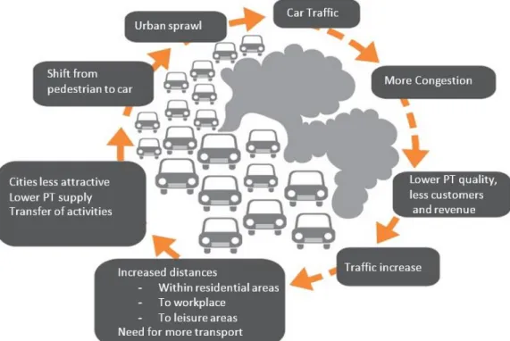
Mobility in networks can be described as the number of movements of individuals between various locations. This is the hardest task in all modelling process, since to obtain accurate quantities of data in this large set isn’t a simple step. A simple way to ratify this problem is to divide the area of interest in different zones and predict the supply and demand generated by each zone. Where the capacity and modes of transportation infrastructures, over a geographically defined transport system, represent transport supply for a specific period of time, to ensure the satisfaction of a certain demand, which is directly affected by the economy advance. A typical example is the vicious circle of urban decline described in the Figure 2.1, which helps understanding the nature of some transport problems.

Economic growth provides the first push to increase car ownership. More car owners means less people using public transport; with fewer public-transport passengers, to which operators may respond by increasing the fares, reducing level of service or both. These measures make the use of the car even more attractive than before and encourage more people to buy cars, thus accelerating the vicious circle. Moreover there is a more devious effect in the long term, illustrated in the Figure 2.1, as car owners chose their place of work and residence without considering the availability of public transport, will generate urban sprawl, low density developments that are more difficult and expensive to serve by more efficient public transport modes. Through the representation in Figure 2.2, we can also understand what can be done to slow down or reverse this vicious circle.

Figure 2.2 – Breaking the car/public-transport vicious circle.

Car limitation, and in particular congestion charging can help to reduce car use and generate profits that can be distributed to other areas of need intervention in urban planning, implementation of traffic schemes, limiting car use in city centers, controlling parking and developing pedestrian zones. Represent some of the measures that can be taken to amend poor or complete lack of traffic planning.

However, the type of model behind Figure 2.2, is not exempt from risks when applied to different contexts. So the context is also pertinent when looking for solutions; it has been said that one of the main objectives of introducing bus-priority schemes in emerging countries is not just to protect buses from car-generated congestion but to organize bus movements. High bus volumes, imply that they will have priority over other cars, which will generate interference between buses and will occur major source of delay than car-generated congestion.

It should be clear that it is not possible to characterize all transport problems in a unique universal form [1]. Transport problems must be always approached as context dependent and so should be the ways of dealing with them. Models offer a contribution in making the identification of problems and selection of ways to address them more solid based, but is obligatory to study case by case.

2.4. D

To effectively do transportation planning it is important to have large amounts of data and cooperation between transportation planning agencies. Advances in technology and the increasing availability of geographic information systems (GIS), are giving transportation planners the facility and ability to advance and use data with a much higher degree of competence. However as mentioned in [8], for information systems to advance, it is essential to provide real data integration/exchange protocols and ways to reduce redundancy and data collection costs. Data compatibility, data access, data quality, metadata, data completeness, hardware, software, and staff expertise are some of many factors that influence the effectiveness of data exchange and data integration efforts.

2.4.1.

M

The OD-matrix describes a network, directed and weighted, and in general is time-dependent. These matrices are usually extremely difficult and costly to measure, and it is only recently, thanks to technological advances such as the global position system (GPS) or the democratization of mobile phones together with geographic and social applications, that help to obtain precise quantities on large data sets, opening the door to an improved reckonable understanding of urban movements.

Calls from cell phones are an additional source of mobility data. Is large enough the density of base stations of antennas, that can serve the mobile phone network in urban areas, so that triangulation gives a relatively accurate indication of the users' position (mobile phones are frequently in contact with the base station; triangulation lets determine the location of the device at a resolution that depends on the local density of base stations). Mobile phone data has lately been used to point individual trajectories [10], to identify ‘anchor points’ where individuals pass most of their time [11-13], or statistics of trip patterns [14-18].

GPS is one more fascinating tool in order to categorize individual trajectories. GPS data of individual vehicles show that the total daily length trip is exponentially dispersed [19, 20], and looks to be independent of the structure of road network, directing to the reality of require more general principles governing human movements [21].

In another scale and even at the scale of social networks, Radio Frequency IDentification (RFID) might offer interesting visions. This technology is usually composed of a tag which can interact with a transceiver that processes all information confined in the tag. RFIDs are used in many different cases, from tagging goods or dynamical measures of social networks [22]. Was also found that the traffic is generally distributed, in arrangement with many other transportation links [7], but also that the displacement length distribution is peaked. However, there is need to keep in mind that there are some problems connected with those methods, such as the present privacy issues, which need to be handled carefully.

To measure the trip-making it is necessary to conduct travel pattern surveys, these may be described in terms of who is going where, with whom, at what time, by which mode of transport and route, and for what purpose.

Surveys represent the largest and most comprehensive source of travel data. Each of the previous types of data collection methods has the shared characteristic that it tries to measure the movements flow. The ability to visualize plus forecast future changes in the system is an important part of the planning process. In particular, as a result of changes in the physical system or changes in the operating characteristics of that system the planner is often required to predict the consequential changes in travel demand. Also it is well predictable that various groups in the population will react differently to changes in the transport system, which it is important to consider when trying to minimize the collateral effects that may be formed in attempting to predict the demands which will be placed on a transport system. To categorize these groups, it is necessary to combine demographic and socio-economic surveys within the complete transport survey framework [23]. As we may also need to understand, each entity reacts not to actual changes in the transport system but to perceived changes in that system. For that reason, perception and attitude surveys often are a vital component of transport planning surveys. Therefore data from surveys are habitually used as inputs to travel demand models. In many cases, a transport survey will realize more than one of the above discussed roles.

2.5. T

Trip generation aims at predicting the total number of trips generated and attracted to each zone of the study area by an O-D matrix or by considering the factors that generate and attract trips, a Production-Attraction (P-A) matrix.

In general we can say it’s a main resource for determining how many vehicle trips will be added to surrounding roadways as a result of new development. The study of trip generation allows to collect and analyze data on the relationships between trips attracted and produced to and from a development, as well as the characteristics of a determined land. It provides trip rates, equations and data plots based on traffic counts and characteristics of the surveyed land uses. The trip rates are appropriate for planning purposes and traffic impact studies.

Some of the models based in an origin destination matrix are suitable for short-term, tactical studies where there aren’t further changes in the accessibility in the network. The P-A are more indicated to when is applied changes in network costs or in tactical studies, that involve important changes in transport prices and are suggested for longer-term strategic. Distribution is often seen as an aggregate problem with an aggregate model for its solution, most of it treatment in this dissertation shares that view.

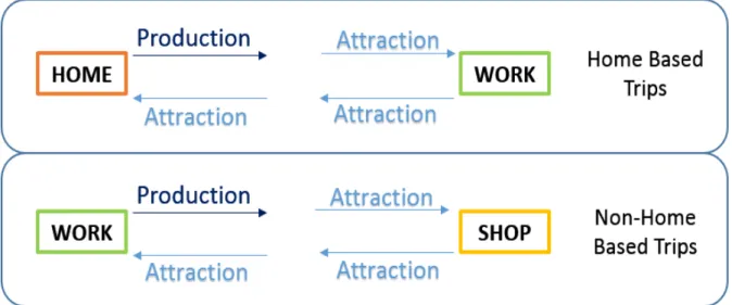
Trip production is defined as, all trips are home based or non-home based as the origin of the trips. In Figure 2.3, trips can be classified by trip purpose, trip time of the day, and by person type.

Figure 2.3 – Trip types.

At the zonal level, it is significant zonal employment and accessibility in trip generation. Being able to model personal trips, freight trips are also of interest. Nevertheless, we should not forget pedestrians, the number of walking trips in denser areas has been more, and therefore those trips must be separated from vehicular ones.

The decision to travel for a given purpose is called trip generation. The trip distribution is the organization of trip generation in a trip matrix, which stores the trips made from an origin to a destination during a particular time period, and may be disaggregated by person and type and purpose of perhaps the activity undertaken at each end of the trip. Thus, trip distribution is a model of travel between zones-trips or links with the purpose to produce a trip table of the estimated number of zones-trips within the study area, estimated by the trip generation models. The modeled trip distribution can then be compared to the actual distribution to see whether the model produces a reasonable approximation.

Different distribution models have been proposed for different sets of problems and conditions, five different models are presented here. These are Growth factor method, Gravity model, Intervening opportunities model, Choice model, and Entropy Model.

2.5.1. G

Given an matrix of trip distribution, and if the only information available is about a general growth rate for the whole study area, then we can only assume that it will apply to each cell in the matrix, that is a uniform growth rate and usually are assumed inflows equal to outflows. Advantages are that they are

simple to understand, and they are useful for short-term planning. Also we can use different types of growth factors, such as: Uniform Factor, Average Factor, Detroit etc. It is a pretty much two step exercise, first we must find the growth factor and lastly apply the factor to all current flows. Limitation is that the same growth factor is assumed for all zones as well as attractions.

2.5.2. G

This model originally generated from an analogy with Newton’s gravitational law. In gravity model, we start from assumptions about trip making behavior and the way it is influenced by external factors. An important aspect of the use of gravity models is their calibration.

The gravity model assumes that the trips produced at an origin and attracted to a destination are directly proportional to the total trip productions at the origin and the total attractions at the destination. The calibrating term or "friction factor" (F) represents the reluctance or impedance of persons to make trips of various duration or distances. The general friction factor indicates that as travel times increase, travelers are increasingly less likely to make trips of such lengths. Calibration of the gravity model involves adjusting the friction factor. The socioeconomic adjustment factor is an adjustment factor for individual trip interchanges. An important consideration in developing the gravity model is "balancing" productions and attractions. Balancing means that the total productions and attractions for a study area are equal.

Before the gravity model can be used for prediction of future travel demand, it must be calibrated. Calibration is accomplished by adjusting the various factors within the gravity model until the model can duplicate a known base year’s trip distribution. For example, if you knew the trip distribution for the current year, you would adjust the gravity model so that it resulted in the same trip distribution as was measured for the current year.

2.5.3. I

The intervening opportunities model, or more briefly, the opportunity model his, like the Gravity model uses the idea of trip making but is not explicitly related to distance but to the relative accessibility of opportunities for satisfying the objective of the trip. The original proponent of this approach was Stouffer (1940), who also applied his ideas to migration and the location of services and residences. But it was Schneider (1959) who developed the theory in the way it is presented today.

2.5.4. C

It is the viewing of urban travel behaviour in a choice framework instead of the traditional demand method, appropriated for describing small areas of traffic behaviours as in micro simulations. Route choice modelling is critical in traffic sub networks approach, designed to be behaviourally realistic. Uses a set of data usually acquired by GPS or the traditional traffic counts, relatively a period of time specified. Mode choice may be influenced by three main groups: characteristics of the trip maker, characteristic only of the journey and the characteristics of the transport facility.

In an aggregate view we have Modal split models that are applied after the gravity or other distributions models, this has the advantage of facilitating the inclusion of the characteristics of the journey and the alternative modes available to undertake them. So this conventional sequential methodology requires the estimation of relatively well defined sub-models. An alternative approach is to develop directly a model subsuming trip generation, distribution and mode choice. This can be of two types: purely direct, which use a single estimated equation to relate travel demand directly to mode, journey and person attributes; and a quasi-direct approach which employs a form of separation between mode split and total O-D travel demand.

To disaggregate choice model we have the multimodal logit model, this is the simplest and most popular practical discrete choice model [26]. Where the ratio of one probability over the other is unaffected by the presence or absence of any additional alternative in the choice set, this means any of two alternatives have a non-zero probability of being chosen.

2.5.5. E

M

There are several possible classes of gravity model specifications, increasing the number of theoretical advantages and there isn’t lack of suitable software to calibrate and use it.

2.6. M

It is acknowledged, that the current transportation modelling process is challenging, in the sense that it employs a great deal of data to a large number of consistent models with many parameters [27]. The complexity of the modelling process, however, it does not exceed the difficulty to acquire accurate representation of complex economic and social phenomena.

The difficulty to analyze or even to represent the uncertainty that characterizes transportation systems and traveler decision making, is overcome with the estimation of many data amounts used.

Before choosing modelling approaches, the follow aspects must be take into account when specifying an analytical approach:

 Precision and accuracy;

 The adaptation of a particular perspective and choice;  Level of detail required;

 The availability of suitable data;  Resources available for the study;  Data processing requirements;

 Levels of training and skills of the analysts;  Modelling process and scope;

Trip-based models are as well-known as the classic transportation model or the conventional four-step modelling process, presented in the following Chapter 3.2 of this Dissertation. They are currently the most universal groups of models used. The trip based approach uses individual trips as the unit of analysis. Time-of-day trips is modelled in a limited way often by applying time-of-day factors to 24 hour travel volumes or is either not modelled.

The parameter trip is the base of analysis in separate models for home-based trips and non-home based trips where is not considered the dependence among such trips. The organization of trips is not considered, there is no distinction between a single trip between origin and destination home-based from a home-based trip with multiple stops along the way, although the impact of such multiple stops has proven to be significant in the local environment. The theoretical challenges of these models, such as developing the algorithm for the user equilibrium approach, have basically been solved by the early 1980’s [28].

Activity-based models have been developed somehow as a response to a change in weight from the evaluation of long term investment based capital improvement strategies, to understand travel behaviour responses in a shorter-term congestion management procedure. Focusing on a set of activity patterns rather than an aggregated trip rate per household, these models try to model a comprehensive daily activity-travel pattern for individuals. This enables the modeler to adjust plans in response to temporal and spatial constraints, also allowing activity rescheduling, trip chaining and destination substitution, one example is the micro simulation models when used as input into a dynamic assignment model the model replaces the generations, distribution and mode choice components and produces dynamically specified trip tables [28].

Several practical aspects of activity-based modelling need to be considered. It needs time, survey data and decision making criteria for analysis and forecasting, consequently requiring the collection of data regarding all activities done by individuals over the course of the day. Although it is similar to administrating household surveys, one need to collect in-home as well as out-of-home activities. Therefore the information required is a little more extensive, but experience suggests that the results are not significantly different between travel surveys and time-use, while at the same time provides a much more comprehensive understanding of travel patterns and trip making.

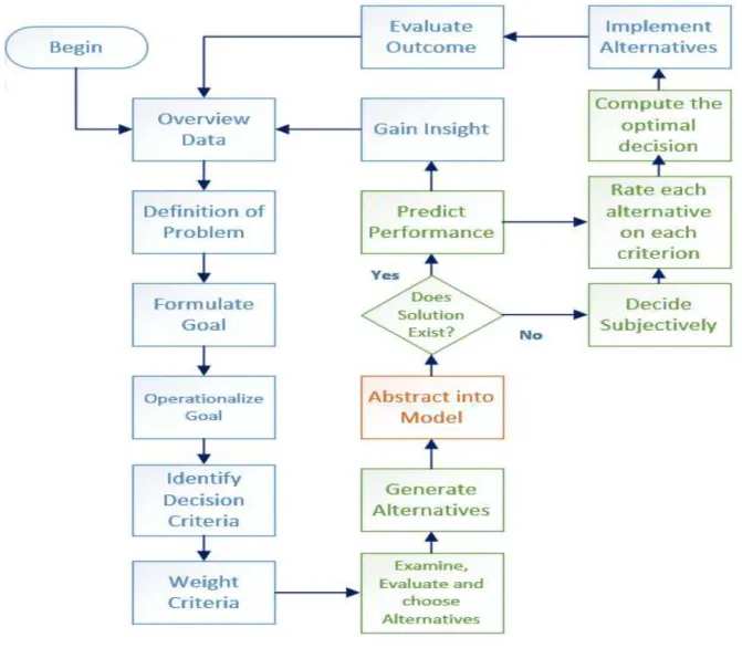
The most prominent decision-making process to emerge from systems analysis is rational planning. The Figure 2.4, illustrates how this system works. We can identify three layers of abstraction. The first layer (green) describes the high level, often unquantified objectives, intermediate goals and immediate actions or experiments, which is summarize in six steps. A second blue layer details many of the components of the first layer. A third layer, identified by the orange box, "abstract into model” depends on the problem at hand.

Figure 2.4 – Rational planning.

3

3.

MACROSCOPIC SIMULATION

3.1.

I

Macroscopic models simulate traffic flow, taking into consideration the several traffic characteristics, flow, speed, and density, but considering their relationships to each other. They can be used to calculate the spatial and sequential extent of congestion caused by traffic demand or incidents in a network, but, they cannot model the interactions of vehicles on alternative design configurations. The simulation in a macroscopic model rather take place on a section-by-section basis than by tracking individual vehicles. Macroscopic models employ equations on the conservation of flow and on how traffic disturbances broadcast through the system like shockwaves [29]. These models were originally developed to model traffic on distinct transportation sub networks, such as corridors including freeways and parallel arterials, surface-street grid networks, and rural highways.

To model and calibrate the road network in analysis we used the program VISUM, a traffic modelling

software belonging to the German company of Transport Planning and Analysis of Operation. VISUM is a complete and flexible software system that contemplates transportation planning, network data management and travel demand modelling. VISUM is used on all continents due to a wide range of planning applications possible such as, metropolitan, regional, state wide and national. The program is designed for multimodal analysis, integrating all relevant modes of transportation into one reliable network model. VISUM provides a variety of assignment procedures and a 4-stage modelling component which includes trip-end based and as well activity based approaches [30].

Our goal for this model is to judge whether the transport system can cope with the predicted passenger volumes, in particular regarding the frequency of the bus company.

3.2.

T

-

This model was developed during the 1950s and 1960s for planning the major highway facilities [31], and soon the model was applied in other traffic planning situations and recognized as a standard for macroscopic modelling.

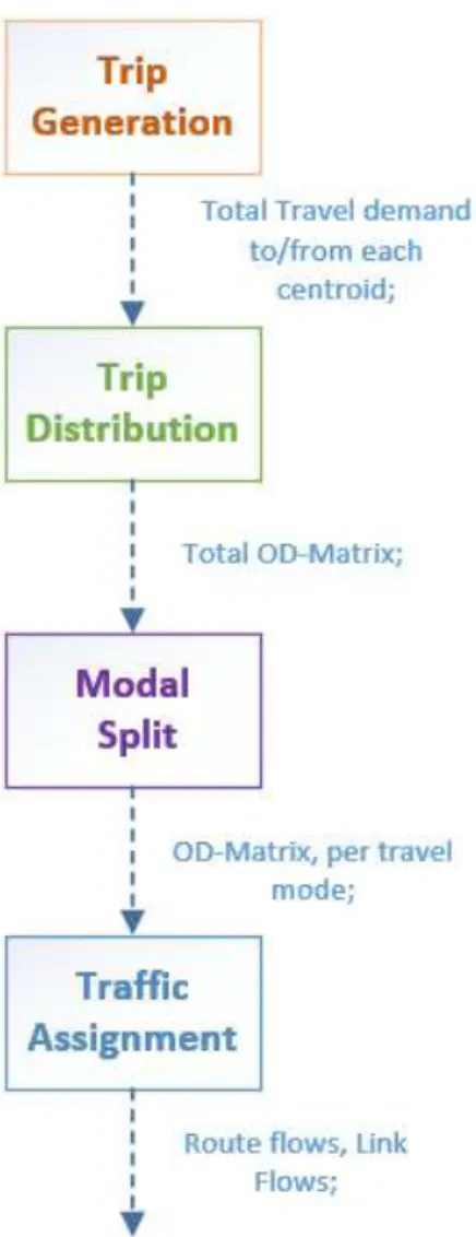
The Figure 3.1 represents the traditional model that follows four sequential stages: Trip generation, Trip distribution, Modal split and Traffic assignment, and depending on the situation, some stages might not be applicable.

Although the four-stage model is almost fifty years old, it is still fundamental for strategic traffic planning. The outcome is, however, always a static description of the situation, which does not provide any information on how the traffic fluctuates over time. To have a time-dependent (dynamic) model we had to consider the influence from traffic conditions in a certain time period where in the traffic assignment model not only the route choice and the resulting route flows must be described for the time period studied, but also the interaction in time between vehicle streams.

The four-stage model and the basic ideas in each of its stages, for the dynamic models is more unexplored in comparison to the static assignment models. Though the first models for dynamic traffic assignment were proposed around thirty years ago [32], there is still no standard model framework. The time-dependent models are also unexpectedly poorly described in books and articles. Two exceptions are the literature overview by Peeta and Ziliaskopoulos (2001) and the basics on dynamic modelling given by Han (2003).

3.2.1.

T

The first stage is Trip Generation, with the aim to determinate how many trips there will be originated or terminated at each zone in the network. The size of these zones in the study zone must be defined with an appropriate accuracy in respect to the purpose of the traffic model. Each zone is represented by a single node in the model which we will refer to as a centroid. To execute this phase it was necessary to collect a variety of data, concerning the characteristics of the trip makers for each centroid, such as age, sex, income, auto ownership, trip-rate, land-use, and travel mode. In general it is a major project to collect the required data, in our study this data was provided by the company Horários do Funchal.

3.2.2.

T

The second stage is trip distribution, where we determine the flow of roads between origin and destination for all trips that were developed in trip generation. Trip distribution uses those trips to and from and independentvariables on the transportation system to forecast the flows/trip interchanges between geography areas. The considerations are in total trips that begin in the first zone, the number ending in the second zone, and the factors that directly influence the impedance or difficulty to travel, such as cost or time between them.

3.2.3.

M

This third stage modal split or known also as modal choice corresponds to the travel demand for each OD-pair and is partitioned into different travel modes. In our case there are only two travel modes available: private car and public transport. In some situations also the purpose of the trip is considered, since, for example, it seems more likely that a person would choose to travel to his work with the public transport, but prefer a private car, if available, for social trips. Further, the purpose of the trip can be important since it might affect the acceptance for a delay or route guidance information. Besides the consideration of available modes and trip purpose, some models also consider the socioeconomic status of the trip-maker. For some people, the travel time is more important than the travel cost, whereas the situation is the opposite for some others. In a simple way the description of the modal split stage is, given the travel demand for each OD-pair, the modal split procedure determines how this volume is disaggregated into different travel modes.

3.2.4.

T

The fourth and final stage, in the traffic assignment the OD-matrix for each mode is assigned onto the traffic network, according to some principle. The aim of this procedure is to calculate the link flow volumes. As indicated, each link must be a bearer of one or more travel modes and in the assignment procedure this must be taken into account. There are in general, many possible routes from one node to another therefore the assignment procedure must follow some assumption on how the routes are chosen. The criterion most used is that all travelers are assumed to drive the shortest path. To conclude the description of the traffic assignment stage we can say that given the travel demand for each mode in each OD-pair, the traffic assignment procedure assigns the travelers to routes in the network and predicts the traffic situation in terms of the link flows for all links in the network.

3.3.

N

Accordingly with the four stages model our modulation was sculpted and adjusted with consideration of:

 Study zone;

 Mobility in the zone;

 System of the collective transport;  Links hierarchy;

 Surveys and count post information;  Traffic count;

 Speeds;  Saturation;

3.3.1.

S

The study zone is Funchal one of the ten municipalities that compose the island of Madeira, in Portugal. Madeira has an approximated area of 785 km2_{, with many slopes that influence the zoning in most areas} of the island. According to the Census of 2011, the Autonomous Region of Madeira had 267.785 habitants with a population density of 334.500 hab/km².

The population of Madeira reflects the geographical constraints that characterize it, where in a large part, the population is on the south coast, which led to the definition of two major centers of occupation: Funchal and Machico.

The urban growth of the island was always concentrated around Funchal due it geographic, with the remaining territory fragmented into clusters. The 90’s is marked by the beginning of population regression phenomena in the municipality of Funchal. These phenomena are typical in polarized urban centers of wide areas, reflecting the urban sprawl movement, where the price of housing is more accessible.

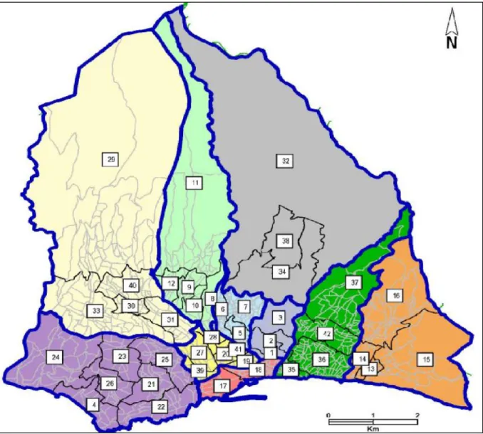
In the Figure 3.2, we can see the 42 zones that compose Funchal and in the Appendix B can be consulted the districts names.

Figure 3.2 – Funchal zone distribuition.

Source: Survey of Mobility in the city of Funchal, 2006/2007.

3.3.2.

M

F

Based on the results of the counts and surveys done to the non resident population , but that performs activities in the study zone, it is estimated that daily "go in" Funchal approximately 24.6 thousand people, which perform about 60.3 thousand trips with end or start in Funchal. The duration of the trips varies, according to the factors considered. By analyzing the transport mode as function of the travels performed internally to city, or the travels generated from others cities to the study area, was possible determinate the average time of these travels. The results are shown in Table 3.1:

Table 3.1 – Average duration of travels: Total and by typology of movement. Source: Survey of Mobility in the city

of Funchal, 2006/2007.

Segment

Travels inside Funchal

Travels to/from Funchal IT 18,4 min 23,7 min PT 24,7 min 44,1 min

On-Foot 19,7 min 14,0 min

TOTAL 20,7 min 30,7 min

3.3.3.

S

The public transport network of Funchal is based mainly on heavy road passenger transport: city and intercity bus networks. The exploration of the road transport service of passengers within the limits of Funchal is the responsibility of a single operator, the company Horários do Funchal.

This is composed by three types of trips:

 Regular journeys, moving generally from the center of Funchal or another destination within the city limits;

 Journeys of high areas, which serve locations with difficult access through special vehicles to rough terrain;

 Journeys of the dawn, serving the municipality of Funchal during night period;

3.3.4.

H

The objective is to serve people and the economy, so the hierarchy of the road network is established from the importance of links offering, and culminates in the profile type and operating conditions that the route must submit. Contribute to this, the dimension and importance of urban agglomeration, the capacity of each link, the tourist interest in the area, the economic activities and establishing links with the outside. In this understanding the following levels in the road hierarchy for Funchal were set as:

 Level 1 - Structural Network

Must ensure the main accesses to the city;  Level 2 - Primary Distribution Network

Should guarantee the distribution of the largest flows of traffic in the city, as well as average routes and access to 1st level;

 Level 3 - Secondary Distribution Network

Must ensure the next distribution, as well as the routing of traffic flows to routes of higher education;

 Level 4 - Network Proximity

Composed of structural pathways of neighborhoods, with some flow capacity;

In the Figure 3.3 we can see which routes were considered in this project.

Figure 3.3 - Classification of the road network by hierarchical level.

3.3.5.

S

For the characterization of the resident population mobility in Funchal were conducted household surveys to residents and telephone surveys to the non resident population. These surveys cover the winter of 2006/2007 and part of the 2007 spring. In a total 3,105 valid surveys were conducted which allow characterize the mobility of the population living in the study area.

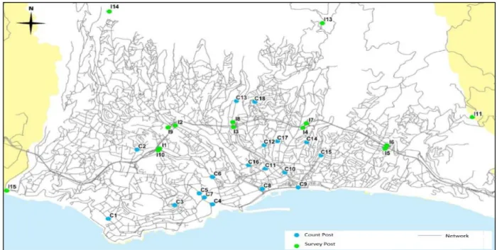
The count post were attributed based on the importance socio-demographic of the area, the road network that serves, and the network of public transport to serve. This lead to this data distribution map shown in the Figure 3.4:

Figure 3.4 – Data Post Locations.

Source: Survey of Mobility in the city of Funchal, 2006/2007.

3.3.6.

T

Therefore the macro and micro simulation models were made to the afternoon peak period, between 18:30 min until 19:30 min, shown in the Figure 3.5, as the highest peak hour of the day:

Figure 3.5 – Progress of traffic in the sum of all the counting stations.

Source: Survey of Mobility in the city of Funchal, 2006/2007.

3.3.7.

S

To measure the road speed practicable in the network was used the GPS technology was used. This allows us to measure with great accuracy the average velocities practiced in the network. It was observed that the highest speeds were recorded in the arcs of higher hierarchy, and as expected the central area of the city offers reduced speeds of circulation, due to concentration of traffic and others factors.

The velocity of circulation is the indicator commonly used to evaluate the performance of a road network, since it allows a direct comparison between the different arcs that constitute the network. The velocity of circulation is calculated based on the theoretical velocity of circulation, which is influenced by the volume of traffic flowing on the road, becoming more significant aggravated as the volume of flow approaches the capacity of the circulation route.

Aside the known congestion problems caused by the under sizing of the roads, the loading and unloading of goods, when occurs for long periods of time causes troubles in the traffic normal circulation. Also the parking maneuver in the parking lots next to some of the roads existent in Funchal affects directly the traffic behaviour.

Figure 3.6 – Average Velocities.

Source: Survey of Mobility in the city of Funchal, 2006/2007

3.3.8.

S

The configuration and performance of the road network were also measured through the degree of saturation of their arteries. The network saturation occurs when the traffic received is more than can be routed. This is a phenomenon that appears when the number of vehicles received, approaches the maximum capacities that each network has. In the peak afternoon hour, we have areas, where traffic exceeds 75% of the maximum capacity of the route, and saturations above 100% corresponding to a conditioned and highly unstable circulation. This means, the volume of traffic exceeds the capacity of the artery causing the formation of queues and stop-start waves.

3.4.

P

I

From the Mobility Study of 2006/2007 was possible for us to have reliable data and a comparable set of network performance indicators. With additional tools to the program from PTV VISSION was possible to determine key performance indicators for traffic management and intelligent transport system included in the model. Cities today face many common transport problems and implement similar urban traffic management solutions, with ITS playing a prominent role. These indicators are important to

3.4.1.

A

W

T

O

The average time that the customer has to wait to enter the public transport system, in areas where the supply is less, the waiting time increases, as are the cases of the north areas Monte, Santa Maria Maior and São Gonçalo. However in coastal and central areas the waiting time is relatively short, not exceeding 5 minutes, while the upland areas can sometimes exceed 7 minutes.

3.4.2.

A

S

M

Is an indicator that evaluates the relationship between the distance traveled, and the time spent on realization of the trip. The average speed of travel, to the trips started in Funchal is generally 9.0 km/h, presenting a minimum of around 6.5 km/h in central areas of São Roque and Imaculado Coração de Maria.

3.4.3.

A

T

S

It matches the speed of the route between the stops, including the times of overflow, which allows the evaluation of the speed of the transport system.

On average moving speed of travel of public transport began in Funchal is 16 km/h. It appears however that the trips started in the city center, have considerably higher average speeds of around 18 km/h, since mostly correspond to long distance trips that split to several axis with commercial speeds. In generally, it is observed that the trips initiated in the western part of the county have higher speeds than trips started in the central and eastern areas.

3.4.4.

A

N

T

3.4.5.

The percentage of direct travel, allow us to judge, to what extent the current network meets the mobility needs of each zone. In a convenient way, identifying connections where supply system is satisfactory, and calculating to what extent it is justified the introduction of more direct connections between certain areas. The areas with the biggest problems are the zones 1 and 4, where the percentage of direct travel is less than 25%. However, despite the area 4 present a low percentage of direct travel, this area recorded one of the largest volume demand. In overall, it appears that more than half of the areas where the trips started, experience more than 75% of direct travel, and there are even several cases where all journeys started, correspond to a direct travel.

3.5.

N

With base on the above parameters was possible to calibrate a macro simulation model to Funchal. The OD-matrix estimation problem amounts to finding a trip table which, when it is assigned onto the network, induces link flows close to those which have been observed in tra_ffic counts. To update our initial O/D matrix with data of 2006/2007 we used VStromFuzzy (Figure 3.7), this tool allows the correction of a given matrix in such a way that the result of the assignment closely matches the latest figures.

Figure 3.7 – VStromFuzzy method.

3.6.

B

F

The correct planning and management of a public transport system can provide a competitive structure with the private motor cars and an efficient coverage of the space of the territory. When attracting travelers from others modes of transport, we are reducing the traffic congestion and obtaining derived benefits like road safety and lower atmospheric and noise pollutions. As seen in the report lent by Horários do Funchal there is a detected frequency problem in this company system.

The correct design of fleet size, routes, timetables and frequencies are primordial for the efficient management of resources [33].

The in-vehicle travel time becomes shorter when the buses have to stop at fewer places, because the distance between bus stops increases and the distance on foot between them too. The opposite is true if the distance between stops is reduced, access time to them is also reduced, but the buses have to stop in more places causing an increase in overall journey time [34]. The bus stops location, accessibility and an attractive overall journey times, are especially important when modifying one public transport system in a city. All of which has direct influence on the size of the fleet and the frequencies within the system. This work proposes an optimal timetable model to minimize the social cost of the overall transport system, taking into account that our demand is constant, we considered congestion on buses, interaction with private traffic, and operational variables (fleet, frequency, operator budgets).

A heuristic algorithm is introduced to solve this problem which, starting from a current feasible solution arrives at a solution which minimizes the overall social cost.

3.6.1.

P

Based on the article [35], a mathematical bi-level optimization model [36], is proposed to answer the problem of bus frequencies because with a bi-level equation we can equilibrate both terms in order to obtain the results proposed. The lower level includes a Mode Choice – Assignment Model [37], and takes into account the influence of private traffic and congestion on the public transport vehicles [38]. An upper level minimizes a cost function both for the user and the operating company [39].

Their formulation is a follows:

where,

TAT Total access time

TWT Total waiting time

TIVT Total in-vehicle time

TTT Total transfer time

TCTT Total car travel time

𝜙𝑎 Value access time

𝜙𝑤 Value of waiting time

𝜙𝑣 Value of in-vehicle time

𝜙𝑡 Value of transfer time

𝜙𝑣′ Value of car travel time

The direct costs are made up of three factors: personnel costs (CP), hourly costs due to standing still with the engine running (CR), rolling costs (km covered) (CK) and fixed costs (CF). The operator’s costs are taken to be the sum of all the direct costs (DC) plus the indirect costs (IC). Others studies have shown that the indirect costs (exploitation, human resources, administrative-financial, depot and supplies, management and general costs) tend to be about 12% of the direct costs. The total cost of the kilometers covered will be equal to:

where _𝐿𝑙= length of route l (km per bus), _𝑓𝑙= frequency of route l (bus per hour), _𝐶𝐾𝑘= unit cost per kilometer covered by bus type k (€ per km), 𝛿𝑘,𝑙= mute variable worth 1 if the bus type k is assigned to

route l and 0 if not.

The personnel cost is found by:

where _𝐶𝑝= is the unit cost per hour of the staff (€ per hour), _𝑡𝑐𝑙=is the time of a round trip (min), _ℎ𝑙= is the headway on route, l (min) = 1/_𝑓𝑙, _{∑ (𝑡𝑐𝑙 𝑙/ℎ𝑙)}= fleet size (bus).

𝑈𝐶 = 𝜙𝑎𝑇𝐴𝑇 + 𝜙𝑤𝑇𝑊𝑇 + 𝜙𝑣𝑇𝐼𝑉𝑇 + 𝜙𝑡𝑇𝑇𝑇 + 𝜙𝑣′𝑇𝐶𝑇𝑇

𝐶𝐾 = ∑ ∑ 𝐿𝑙 𝑘 𝑙

𝑓𝑙𝐶𝐾𝑘𝛿𝑘,𝑙

𝐶𝑃 = 𝐶𝑝∑(𝑡𝑐𝑙 𝑙