532
© Author(s) 2007. This work is licensed under a Creative Commons License.
Development of a high resolution grid-based river flow model for
use with regional climate model output
V.A.
Bell
1, A.L. Kay
1, R.G. Jones
2and R.J. Moore
11Centre for Ecology and Hydrology, Wallingford, Oxfordshire, OX10 8BB, UK
2Met Office Hadley Centre (Reading Unit), Meteorology Building, University of Reading, Reading, RG6 6BB, UK Email for corresponding author: [email protected]
Abstract
A grid-based approach to river flow modelling has been developed for regional assessments of the impact of environmental change on hydrologically sensitive systems. The approach also provides a means of assessing, and providing feedback on, the hydrological performance of the land-surface component of a regional climate model (RCM). When combined with information on the evolution of climate, the model can give estimates of the impact of future climate change on river flows and flooding. The high-resolution flow routing and runoff-production model is designed for use with RCM-derived rainfall and potential evaporation (PE), although other sources of gridded rainfall and PE can be employed. Called the Grid-to-Grid Model, or G2G, it can be configured on grids of different resolution and coverage (a 1 km grid over the UK is used here). The model can simulate flow on an area-wide basis as well as providing estimates of fluvial discharges for input to shelf-sea and ocean models. Configuration of the flow routing model on a relatively high resolution 1 km grid allows modelled river flows to be compared with gauged observations for a variety of catchments across the UK. Modelled flows are also compared with those obtained from a catchment-based model, a parameter-generalised form of the Probability-Distributed Model (PDM) developed for assessing flood frequency. Using RCM re-analysis rainfall and PE as input, the G2G model performs well compared with measured flows at a daily time-step, particularly for high relief catchments. It performs less well for low-relief and groundwater-dominated regions because the dominant model control on runoff production is topography.
Keywords: flow routing, DTM, hydrological model, regional climate model, flood frequency
Introduction
Analyses of rainfall estimated by climate models have indicated changes in the characteristics of extreme precipitation over Europe under enhanced greenhouse gas climate conditions (Giorgi et al., 2001). Specifically, an analysis of rainfall from different climate models indicates a consensus for wetter winters in northern Europe and drier summers in southern Europe (Hulme et al., 2002). A detailed assessment of output from a range of Regional Climate Models (RCMs) by Giorgi et al. (2001) indicates an increase in the frequency of precipitation events exceeding 30 mm day1
. Prolonged and widespread flooding over northern Europe in recent years has raised the question of the likely effects of changes in precipitation on hydrological regimes and, in particular, the effect on flood frequency and severity. To examine the likely impact of future climate change on river flows, typical studies have applied the output from
climate models to catchment-scale hydrological models as changes to the baseline-observed climate. Kay et al. (2006) review current methods and show how RCM atmospheric variables can be used as input to a rainfallrunoff model for individual catchments across the UK. The apparent skill of RCMs in estimating current rainfall extremes (Huntingford et al., 2003; Fowler et al., 2005) gives some confidence in their estimation of extreme rainfall under future climate conditions. Improvements in the resolution of RCMs now provide a basis to examine, systematically, how any change in precipitation characteristics will affect hydrological regimes.
533 (DTM) data. The scheme provides a simple modelling
framework which can translate climate model estimates of current or future scenarios of rainfall (and potential evaporation) into estimated river flow at a daily/sub-daily time-step. The scheme is of potential value in many ways. Firstly, it can provide planners with regional, area-wide estimates of future changes in river flow and flood frequency. Secondly, its simple grid-based configuration allows it to be coupled directly with climate models, land-surface schemes and ocean models (e.g. Lucas-Picher et al., 2003). Also, it is in the nature of catchments to integrate rainfall, soil water and runoff fluxes spatially to form river flow which can be measured routinely and used for model assessment. Thus, thirdly, through comparison with river flow measurements, the routing scheme provides a spatially-integrated method of assessing the soil-moisture accounting and runoff-production components of land-surface schemes for which observational data are not available routinely and which involve quantities that are highly variable in space.
Model overview
INTRODUCTION
Flow routing is being used, increasingly, to diagnose the output from large-scale land-surface models and Global Climate Models through reference to observations of river flows (Aroro and Boer, 1999; Hagemann and Dumenil, 1998; Miller et al., 1994; Oki et al., 2001; Sausen et al., 1994; Yu et al., 1999). Such diagnostic studies typically produce monthly estimates of river flow and can provide estimates of the freshwater input to ocean models, possibly as part of a fully coupled atmosphere-land-surface-ocean model.
Recent increases in the resolution of RCMs (25 km is used here) and ocean/shelf-sea models have increased the possibility and demand for more detailed estimates of river flow. This, in turn, has reduced the difference in scale between detailed hydrological models (estimating flow at sub-daily time-steps) and broad-scale land-surface and river flow routing models. Coupled atmospheric-hydrological models such as the variable flow-routing scheme of Lucas-Picher et al. (2003) in the Canadian RCM and the RiTHM model (~25 km resolution) of Ducharne et al. (2003) have already demonstrated the utility of such schemes for modelling monthly streamflow and for validating atmospheric models.
The Grid-to-Grid (G2G) model was developed to investigate the feasibility of using a higher-resolution (1 km × 1 km) grid-based river-flow routing model for large/ regional domains in simulating daily or sub-daily river flows.
Such detailed output is increasingly required for studies into the effects of climate change on small to medium catchments (say, from 5 to 10 000 km2
in area), and for studies into dependencies between sea-surges and extreme river flows. The G2G flow routing scheme uses gridded estimates of runoff provided by a simple grid-based runoff-production scheme developed from the CEH Grid Model (Bell and Moore, 1998). Flow-routing along land and river flow paths delineated by a DTM is used to propagate grid-square estimates of runoff laterally to estimate flow at points along a river as well as discharges to the sea. The simple modular nature of the algorithm means that any land-surface scheme could eventually provide gridded runoff estimates taking into account the effect of spatially-varying properties of the topography, soil, land-cover and geology.
The G2G model is assessed here with reference to daily flow observations for selected UK catchments. Its performance is also compared with that from an alternative model, the parameter-generalised PDM, a form of catchment-based rainfallrunoff model tailored for use in deriving flood frequency curves via continuous simulation of river flow (Calver et al., 2001; Lamb et al., 2000; Kay et al., 2003; Kay, 2003). The inclusion of this catchment model provides an opportunity to assess the relative strengths and weaknesses of lumped catchment and area-wide grid model approaches to flood estimation.
THE G2G ROUTING MODEL
The G2G flow routing model is based on the discrete approximation to the 1-D kinematic wave equation with lateral inflow; this relates channel flow, q, and lateral inflow per unit length of river, u, by
cu x q c t q
w w w w
, (1)
where c is the kinematic wave speed and t an d x are, respectively, time and distance along the reach. If t and x are divided into discrete intervals Dt and Dx such that k and n denote positions in discrete time and space, then invoking forward difference approximations to the derivatives in (1) gives the discrete formulation
nk n k n k n
k q q u
q 1
1 1
1 T T (2)
where the dimensionless wave speed q = c Dt/Dx and 0 < q
< 1. This is a simple, explicit numerical formulation which has the advantage of introducing diffusion (albeit numerically) and so represents more closely the propagation of actual flow in rivers.
534
equations for gradually-varying flow in open channels has been used in operational flood forecasting systems by Moore and Jones (1978) and Jones and Moore (1980). Such models tend to be configured, manually, to an individual river network (incorporating features such as tributary inflows, floodplain storages and river gauging stations) and to have a number of physically-based parameters which must be adjusted for optimal performance in a particular river reach. Bell and Moore (1998) show how a DTM can support the configuration of the above 1-D kinematic wave model using isochrones to delineate each routing reach within a catchment. A kinematic wave approximation has also been used to model overland flow of water in two-dimensions, using a DTM to derive topographic information and flow-directions (Singh, 1996; Jain and Singh, 2005).
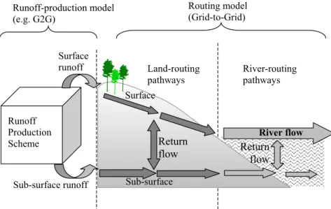
The simple kinematic wave scheme of Eqn. (1) has been used to develop a 2-D G2G formulation for routing both land and river flows in the G2G Model. It is assumed that a separate runoff-production scheme partitions precipitation and evaporation fluxes between water stored in the soil and canopy and water generated as surface and sub-surface runoff. Following Bell and Moore (1998), kinematic routing is applied separately to sub-surface and surface runoff, whilst also allowing for different formulations over land and river pathways (initially just a different wave speed). A return flow term allows for flow transfers between the sub-surface and sub-surface pathways to represent sub- surface/sub-surface flow interactions on hillslopes and in channels. In river cells, the return flow term provides a spatially continuous way of combining the fast and slow components of river flow. By way of comparison, in lumped hydrological models such as the PDM, baseflow is generally
added to surface flow only at the catchment outlet. Figure 1 is a schematic of the model structure.
The model equations in 1-dimension are as follows:
) ( ) ( ) ( ) ( r rb rb rb rb rb r r r r r r l lb lb lb lb lb l l l l l l R u c dx q c t q R u c dx q c t q R u c dx q c t q R u c dx q c t q w w w w w w w w w w w w (3)
where ql is flow over land pathways, qr is flow over river pathways, Rland Rr denote land and river return flow, and ul and ur are inflows for land and river, which include runoff generated by a runoff-production scheme. The additional subscript b denotes sub-surface (baseflow) pathways.
The four partial differential equations are each discretised using a finite-difference representation similar to Eqn. (2) but extended to include the return flow term n
k
R , such that:
n k n k n k n k nk q q u R
q 1
1 1
1 T T . (4)
For application to two dimensions, the 1 1
n k
q term, which represents inflow from the preceding grid-cell in space, is given by the sum of the inflows from adjacent grid-cells.
In practice, the routing is implemented in terms of an equivalent depth of water in store over the grid square, n,
k S
with kn
n
k S
q N and where N c/'x is a rate constant with units of inverse time and 'xis the size of the grid-cell. The inflow and return flow are also presented as water depths. Return flow to the surface is given by n
k n
k rS
R where n
k S Runoff-production model (e.g. G2G) Return flow Sub-surface River flow Routing model (Grid-to-Grid) Surface Return flow River-routing pathways Land-routing pathways Sub-surface runoff Surface runoff Runoff Production Scheme
535 is the depth of water in the sub-surface store and 0£r£1 is
the return flow fraction, which represents the proportion of the sub-surface store content that is routed to the surface; it can differ for land and river paths. Note that, whilst return flow is normally positive, it can take negative values to represent influent, rather than the more normal effluent, stream conditions. The flow-routing model formulation allows for different values of the dimensionless wave speed,
t
'
N
T , for surface and sub-surface pathways; it would be
expected to take a larger value for river pathways.
THE G2G RUNOFF PRODUCTION SCHEME
A runoff-production scheme is required to provide grid-based estimates of surface and sub-surface runoff for input to the G2G routing scheme. A simple scheme has been used in the interim until a comprehensive land-surface scheme, under development, is available. This has allowed progress on the new routing formulation which has been the main thrust of the research reported here. The runoff-production scheme is configured on a 1-km grid, and is based on the runoff-production component of the catchment-based CEH Grid Model (Bell and Moore, 1998).
For a given grid square, the following linkage function relates the maximum storage capacity, Smax, and the average
topographic gradient, g, within the grid square:
max max
max 1 c
g g S ¸¸ ¹ · ¨¨ © § , (5)
for g dgmax. The parameters gmax and cmax are upper
limits of gradient and storage capacity respectively and act as regional parameters for the runoff-production model. An estimate of mean slope for each grid square can be obtained from a DTM. In turn, this allows determination of the structural parameter Smax for all grid squares, using only
the two regional parameters, gmax and cmax.
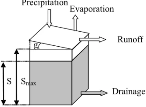
The soil column loses water in three ways. If the column is fully saturated from previous rainfall events, then further rainfall spills over and contributes to the fast catchment response. Drainage from the base of the column is dependent on the volume of water stored in the column; it contributes to the slow response of the catchment to rainfall. Finally, water is lost by evaporation from the top of the column, particularly in summer. Figure 2 illustrates a typical soil column in a grid square and the elements of the water balance in the column.
Specifically, a water balance is maintained for each grid square and time interval (ignoring time and space subscripts for notational simplicity) as follows.
Evaporation loss from the soil column occurs at the rate, Ea, which is related to the potential evaporation rate, E,
through the relation
°¿ ° ¾ ½ °¯ ° ® ¸¸ ¹ · ¨¨ © § 2 max max 1 S S S E
Ea , (6)
where S is the depth of water in store. Drainage from the grid box which contributes to the slow catchment response, occurs at the rate
¯ ® d ! , 0 , 0 , 0 , S S S k d d E (7)
where kd is a storage rate constant and the exponent b is a parameter (set here to 3).
Finally, the (potential) water storage is given by the update equation
(8)
where p is the rainfall rate. The direct runoff rate contributing to the fast catchment response is then calculated as
) ,
0
max( S Smax
q , (9)
and the water storage S reset to Smax if direct runoff is
generated. The inflows to the flow-routing scheme of Eqn. (3), ur or ul, and urb or ulb, comprise the surface and sub-surface runoff terms, q and d, in Eqns. (9) and (7), depending on whether the grid-square is assigned as land or river.
Heterogeneity of soil water storage within a grid square is introduced by a variant on the basic Grid Model scheme which employs a probability-distributed store within a model grid-square. The probability-distributed soil moisture (PDM) formulation developed by Moore (1985) has been applied to an individual grid square. The benefit of introducing this additional level of complexity into the model is that a certain proportion of the grid square is assumed to be saturated and
g Runoff
S Smax
Precipitation
Evaporation
Drainage
Fig. 2. A typical grid-box storage illustrating the components of the water balance.
) ,
0
max( S p t E t d t
536
generating runoff even when rainfall amounts are small; under the basic formulation, an entire grid square would have to be saturated before it generated runoff.
The PDM extension to the Grid Model of Bell and Moore (1998) has been applied as follows. The simple empirical relation between gradient, g, and storage capacity, c, at a point
max max
1 c
g g
c ¸¸
¹ · ¨¨
© §
, (10)
is used to develop a probability-distributed soil moisture storage formulation as an extension to the approach of Moore (1985). Here, gmax and cmax are the maximum point slope and storage capacity values within an area. For a given distribution of gradient within a grid square, Eqn. (10) can be used to derive the distribution of storage capacity over the square in terms of the parameters defining the distribution of gradient. The grid-based scheme requires two parameters to be determined: these are shown in Table 1, together with the values used for the regional calibration.
The PDM part of the runoff production scheme requires a value for b, a parameter which determines the shape of the Pareto distribution used in the soil-store distribution. In the current application, b has been determined from grid-square slope values (Bell and Moore, 1998). A further parameter, cmin, introduces a minimum depth of soil store which has to be filled before runoff is generated. Setting cmin to a small non-zero value (here 0.01 mm) reduces the occurrence of flow peaks generated by very light rainfall.
INITIALISATION OF MODEL STORES
Initial values for flow-routing stores in an operational river flow model can often be inferred from an observation of river flow at a single gauged location. The gridded flow observations that would be required to initialise a distributed grid-based model in the same way are rarely if ever available. A straightforward approach to initialise the river and soil-moisture stores of gridded models is to set them to zero and allow for a period of warm-up. As an alternative, here stores have been initialised based on an estimate of mean annual flow derived using geomorphological relations.
The relationship between mean annual flow and catchment area is usually approximately linear (Leopold et al., 1964). However, for hilly and mountainous regions, precipitation (and therefore runoff) can be highly dependent on elevation, so that the assumption of spatial homogeneity does not apply. Hence, estimates of Standard Average Annual Rainfall (SAAR) have been included in the relationship between mean annual flow, qmean (m3
s-1
) and catchment drainage area, A (km2
), and SAAR, RSAAR (mm), using the relation
341 . 1 058
. 1
1000 0108
.
0 ¸
¹ · ¨ © § SAAR
mean
R A
q . (11)
This relationship was derived from over 1500 values of mean flow, SAAR and catchment area for catchments across the UK extracted from the UK Surface Water Archive.
OVERVIEW OF THE PARAMETER-GENERALISED PDM
In addition to comparison with observed flows, the performance of the G2G scheme is assessed here with Table 1. Runoff-production and routing model parameters.
Parameter name Symbol Units Typical value Description
ROUTINGPARAMETERS: Surface wave speeds:
Land: cl m s
1 0.4 Related to the flow velocity
River: cr m s
1 0.5
Sub-surface wave speeds:
Land: clb m s
1 0.05 Usually less than the surface
River: crb m s
1 0.05 wave speed
Return flow factors:
Land: rl - 0.005 Proportion of the sub-surface store River: rr - 0.005 that is routed to the surface/river
RUNOFF-PRODUCTIONPARAMETERS:
Maximum store depth cmax mm 140. Maximum store depth
reference to flows obtained using a catchment-based
rainfall-runoff model developed for flood frequency assessment by continuous simulation of river flow. This rainfall-runoff model is a simple form of the Probability Distributed Model (PDM; Moore 1985, 1999), the parameters of which have been generalised spatially to allow estimation at ungauged sites, using relationships between the model parameters and catchment properties derived from information on terrain, soil, land-cover and geology. Hereafter, this model will be referred to as the parameter-generalised PDM. Kay et al. (2003) demonstrate how this spatial parameter-generalisation may be used to provide parameters for the parameter-generalised PDM at ungauged locations; by way of background to the application and comparisons that follow, the technique is outlined here.
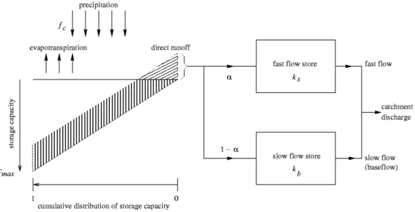
The PDM provides a toolkit of simple model structures that can be applied effectively to a variety of catchment and climate conditions. It is based on conceptual water stores, and non-linearity in the transformation from rainfall to runoff is represented by using a probability distribution of soil moisture storage capacity. This determines the time-varying proportion of the catchment that contributes to runoff, through either fast or slow pathways. The full PDM encompasses many different possible model formulations. Lamb (1999) found that using models with fewer free parameters was advantageous for spatial parameter-generalisation. Whilst fixing the model form and reducing the number of parameters may sacrifice some site-specific performance, particularly in terms of simulated flows, the overall performance for flood frequency estimation when using generalised parameters was found to improve when parameter-sparse models were employed (Calver et al.,
2001; Crewett et al., 1999). The simplified version of the PDM, with five parameters, is used here. A diagram illustrating its conceptual structure is presented in Fig. 3.
Data for model input and model
assessment
PRECIPITATION INPUT
The G2G runoff-production scheme requires as input gridded values of rainfall and potential evaporation (PE). Here, two different sources of precipitation have been used:
(i) 5 km grid-interpolated daily observed rainfall (1958 to 2002) obtained from the Met Office;
(ii) hourly precipitation from a 25 km RCM driven with ECMWF Re-Analysis (ERA) boundary conditions (1979 to 1993).
As an estimate of actual rainfall, the daily source, based on daily measurements from an extensive network of raingauges, can be regarded as good and suitable for model calibration. The hourly RCM source, being model-based and tied to actual time via its boundary conditions, is less good at reproducing observed rain amounts. However, it is this hourly source that will give confidence in the RCM rainfalls under recent climate conditions and, in turn, provide some indicator of performance under future climates, the impacts of which are to be assessed. The RCM source is used, therefore, not for model calibration, but in the assessment of modelled flow predictions. The hourly variability in the RCM rainfall may prove of some additional benefit when
simulating runoff and river flow processes that are sensitive to smaller time-scale variations.
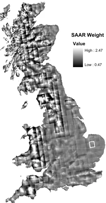
To take account of the higher spatial variability of rainfall at a 1 km resolution, the Standard Average Annual Rainfall (SAAR) 1 km dataset has been used to downscale both types of precipitation data to the 1 km UK National Grid. For the RCM data, for each time-step the rainfall for each RCM grid-square is multiplied by the ratio of the RCM 25 km grid-square SAAR to the 1 km SAAR value, to provide rainfall on a 1 km grid. Specifically, the multiplicative weight for a 1 km pixel at location (i,j), Zij, is calculated as
, ) , (
SAAR SAAR ij
R j i R
Z (12)
where RSAAR(i,j) is the SAAR of the 1km pixel and RSAAR is
the mean SAAR of the RCM grid-cell that encompasses it. The formulation ensures that the total rainfall for the RCM grid-cell remains unchanged. Figure 4 is a map of the 1 km SAAR weights, Éij, for Great Britain; spatial variation in the SAAR weights is greater in areas of high relief to the north and west of Britain and less in the south-east.A similar spatial weighting has been used to downscale the 5 km observed daily rainfall to a 1 km grid; however, no attempt has been made to disaggregate the daily rainfall observations
Low : 0.47 High : 2.47
Value
SAAR Weight
into hourly estimates, other than to divide the daily rainfall
estimates into 24 equal parts.
POTENTIAL EVAPORATION INPUT
Daily PE values are required for both the PDM and the G2G model. RCMs do not output PE data directly, although they do produce actual evaporation estimates as an integral part of their surface-vegetation-atmosphere transfer (SVAT) scheme. Several procedures have been devised to estimate PE from climate data (Shuttleworth, 1993) but the most physically-based and best-established of these is the Penman-Monteith equation (Monteith, 1965). This has been used by the Met Office within the Meteorological Office Rainfall and Evaporation Calculation System (MORECS) for generating a monthly climatological dataset for 201 40 km × 40 km squares across the UK as well as daily site values for synoptic stations (Thompson et al., 1982; Hough et al., 1997). The calculation involves temperature, humidity, wind speed and net radiation. The formulation incorporates the effect of plant physiological properties and, thus, PE
estimates vary with land cover. The standard MORECS PE dataset assumes a grass crop 0.15 m high as is assumed here. PE has been calculated from RCM outputs in a reasonably close emulation of the Penman-Monteith calculation as implemented in MORECS, but using RCM outputs instead of synoptic station measurements. A comparison of RCM-derived PE for two grid-boxes with observed PE from MORECS synoptic sites within those grid-boxes indicates no obvious bias in the RCM-derived PE, either in magnitude or timing (Kay et al., 2006).
For the present application, where the PDM and the G2G runoff-production scheme use an hourly model time-step, daily PE estimates calculated from RCM outputs were converted to hourly values simply by spreading them equally throughout the day. This method is sufficient for PE input, since its effect on runoff production is as a cumulative control on soil water storage. For model simulations involving the 5 km grid-interpolated daily rainfall observations, monthly 40 km MORECS PE data have been used, spread equally over the days and hours in the month.
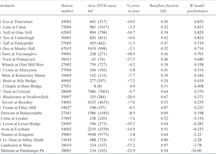
Table 2. R2
performance statistics for daily flows in 25 UK catchments.
Catchment Station Area (DTM area) % error Baseflow fraction R2 model number km2 in area (bfi) performance
18. Exe at Thorverton 45001 601 (517) -14.0 0.50 0.855
15. Lune at Caton 72004 983 (1017) +3.5 0.32 0.833
14. Teifi at Glan Teifi 62001 894 (798) -10.7 0.54 0.829
19. Taw at Umberleigh 50001 826 (831) +0.6 0.42 0.824
25. Taff at Pontypridd 57005 455 (462) +1.5 0.47 0.719
20. Dee at Manley Hall 67015 1019 (998) -2.1 0.52 0.714
13.Tawe at Ynystanglws 59001 228 (271) +18.9 0.36 0.701
11. Yscir at Pontaryscir 56013 63 (74) +17.5 0.46 0.680
4. Wharfe at Flint Mill Weir 27002 759 (727) -4.2 0.39 0.558
12. Cynon at Abercynon 57004 106 (102) -3.8 0.41 0.534
1. Mole at Kinnersley Manor 39069 142 (131) -7.7 0.39 0.444
23. Beult at Stile Bridge 40005 277 (297) +7.2 0.24 0.434
21. Crimple at Burn Bridge 27051 8 (8) 0.0 0.31 0.408
17. Trent at Colwick 28009 7486 (7063) -5.7 0.64 0.376
22. Blackwater at Swallowfield 39007 355 (284) -20.0 0.67 0.371
8. Severn at Bewdley 54001 4325 (4653) +7.6 0.53 0.239
24. Frome at Ebley Mill 54027 198 (197) -0.5 0.87 0.223
3. Derwent at Buttercrambe 27041 1586 (1445) -8.9 0.69 0.198
5. Colne at Lexden 37005 238 (220) -7.6 0.52 0.154
16. Leven at Leven Bridge 25005 196 (273) +39.3 0.44 -0.281
9. Avon at Evesham 54002 2210 (2539) +14.9 0.51 -0.353
2. Thames at Kingston 39001 9948 (9773) -1.8 0.64 -2.22
10. Lt. Ouse at Abbey Heath 33034 688 (724) +5.2 0.80 -2.28
7. Lambourn at Shaw 39019 234 (147) -37.2 0.97 -3.78
RIVER FLOW OBSERVATIONS FOR MODEL ASSESSMENT
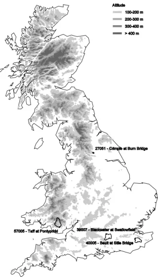
Model performance has been assessed by comparison with flow observations at 25 locations across the UK. The catchments are listed in Table 2, together with their catchment area and baseflow index (bfi) (Institute of Hydrology, 1980); this dimensionless variable (range 0 to 1) expresses the fraction of the river flow that derives from stored sources, such as groundwater. The catchments were chosen to represent a wide range of river regimes, from fast upland catchments (e.g. Taw, Dee) to large baseflow-dominated river basins (e.g. Thames, Little Ouse). It is important to remember that artificial controls on flow, such as reservoirs or abstractions for water supply, are not as yet accounted for in the G2G model. Four of the catchments were selected specifically for comparison with the parameter-generalised PDM model: the Crimple at Burn Bridge (27051), the Blackwater at Swallowfield (39007), the Beult at Stile Bridge (40005) and the Taff at Pontypridd (57005). A map of the UK showing catchment boundaries and locations is presented in Fig. 5. Daily flow data for the catchments in Table 2, originating from the Environment Agency, were obtained from the National River Flow Archive at CEH Wallingford. Hourly flow data for the four catchments used with the parameter-generalised PDM were obtained directly from the Environment Agency.
DTM-DERIVED DATA FOR MODEL CONFIGURATION
The G2G routing model requires three DTM-derived datasets:
(i) flow directions (each grid-cell can drain in only one of eight directions);
(ii) area draining to each 1 km grid-cell;
(iii) standard Average Annual Rainfall (SAAR) for the area draining to a grid-cell;
whilst the runoff-production scheme also requires (iv) average slope.
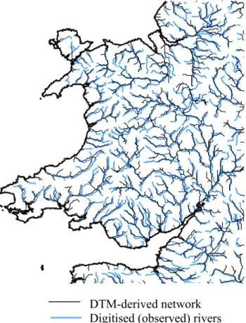
Flow directions for the G2G routing model have been derived automatically at a 1 km resolution using hydrological grid-based tools within the GIS package ArcInfo. The flow directions derived from the HYDRO1K digital elevation data (USGS, 1998) were projected onto the UK National Grid and corrected manually to achieve a digital river network that is as close as possible to that observed on the UK mainland. Figure 6 compares the DTM-Derwent
Thames Wharfe
Mimram Colne
Mole Lune
Severn
Avon
Lambourne
Leven
Tawe Teifi
Cynon Yscir
Lt. Ouse Trent
Exe Dee
Taw
Beult Taff
Crimple
Blackwater
Fig. 5. Location of UK catchments used for model assessment.
DTM-derived network
Digitised (observed) rivers
derived river network for Wales with a map of digitised
rivers. The correspondence at this scale is reasonable though there is clearly room for improvement. Most of the manual corrections were on large rivers, for which a small error could lead to significant errors in modelled flow. There are still numerous errors in flow directions which result in over-or under-estimation of catchment area and flow. A near-perfect set of flow directions would contribute significantly to optimal model performance but achieving this task is time-consuming and was outside the scope of the current project. Fekete et al. (2001) and Olivera and Raina (2003), for example, explore ways of deriving more accurate flow-directions automatically from higher resolution DTM datasets and these methods may be less onerous in achieving an optimal set of flow directions.
The DTM-derived datasets provide the spatial information required by the G2G flow routing model. The accumulated areas dataset that follows from the delineation of the routing paths provides a way of determining whether a 1 km grid-square can be classified as land or river; a threshold drainage area, aT, can be set within the model such that a land/river indicator, xij, for grid-square (i,j) is defined as
¯ ®
t
, ,
, ,
T ij
T ij ij
a a river
a a land x
where aij is the accumulated area draining to the grid-square.
Model calibration
REGIONAL CALIBRATION
The G2G model has been designed for area-wide application, providing estimates of flow for rivers throughout a region, in this case the UK, irrespective of catchment boundaries. In the model, gridded datasets represent the spatial heterogeneity of hydrological response across grid-cells. A few parameters are set at a regional level and are treated as parameters for model calibration. These control the overall runoff response and flow translation of the model and are used, along with the gridded datasets, to derive the grid-cell parameter values.
The model parameters have been adjusted using a range of periods in the three years 1960 to 1962 for which 5 km daily rainfall are available. The gridded daily rainfall has been used for G2G model calibration since, being based on raingauge observations, it is a better source than the model-based RCM hourly estimates, as previously discussed. Daily average flow observations have been used for model assessment partly because of their greater availability but also because use of daily rainfalls as model input limits the value of sub-daily assessment. Whilst the routing model is
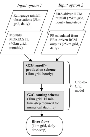
run at a 15-minute time-step, modelled 15-minute flows are aggregated to daily average flows for model calibration and assessment. Model performance at, say an hourly resolution, is, therefore, uncertain, except in terms of the simulation of flow volumes over the day. This is likely to be particularly true for smaller catchments which respond quickly whilst larger catchments which respond more slowly will have average daily flow rates closer to hourly peak rates and will be less sensitive in calibration. Figure 7 is a schematic of the model structure and its inputs and it clarifies the spatial and temporal resolution in use at each stage.
Table 1 presents a single set of routing and runoff-production model parameters for the whole region of application, in this case the UK. The parameters have been adjusted manually to obtain the best match between modelled and observed flows for as many catchments as possible. The sub-surface and surface wave speed parameters can take different values for land and river grid-squares, although this has not been invoked for the sub-surface flows here.
Input option 2 Input option 1
ERA-driven RCM rainfall (25km grid, hourly time-step) Raingauge rainfall
observations (5km grid, daily)
PE calculated from ERA-driven RCM outputs (25km grid, daily)
Monthly MORECS PE (40km grid, monthly)
G2G runoff -production scheme (1km grid, hourly)
Grid-to-Grid model G2G routing scheme
(1km grid, 15 min time-step required for numerical stability)
River flows (1km grid, daily time-step)
542
CATCHMENT CALIBRATION
It is intended that the same set of regional model parameters is applied to all catchments irrespective of their properties (topography, land cover, soil, geology, spatial extent); the aim is to represent such spatial heterogeneity by linking model components to gridded datasets. However, at this early stage of development, the G2G model is not being used with these additional datasets and so it may be at a disadvantage when compared with the parameter-generalised PDM which has been tuned to local conditions with reference to catchment-property datasets. Therefore, to judge how the model could perform if it were tuned to local conditions, the G2G has been calibrated manually on daily flow observations for four catchments. As with the regional calibration, this has been done for a range of periods in the three years 1960 to 1962 for which 5 km observed daily rainfalls are available.
Model assessment
THE ASSESSMENT PROCEDURE
The G2G model has been assessed over the nine year period 1985 to 1993 for which both 25 km hourly ERA-driven RCM (experiment acgxz) rainfall estimates and 5 km grid-interpolated daily observed rainfalls are available. While it is expected that daily rainfall based on observations will provide better flow simulations, the quality of the flow predictions using the RCM hourly rainfalls reflect the possible value of RCM rainfall for climate-change impact assessments.
The G2G routing model is run at a time-step of 15 minutes (required for numerical stability) and at a spatial resolution of 1 km, although the RCM driving data (rainfall and PE estimates) are currently available only at a 25 km resolution.
The model can be run in two modes:
(i) Regional calibration mode: for the whole of the UK with a single set of model parameters, yielding estimates of flow on a 1 km grid over the UK.
(ii) Catchment calibration mode: for an individual catchment, where the parameters have been calibrated to achieve the optimal results for that catchment alone.
The routing model assessed using regional model parameters will be referred to as the regional-calibration, while results obtained using the model calibrated to a particular catchment will be referred to as the catchment calibration.
ASSESSMENT USING (DAILY) RAINFALL OBSERVATIONS
This assessment uses the best available rainfall data for both the parameter-generalised PDM and the G2G model. These comprise hourly catchment rainfall based on raingauge measurements for the PDM and daily raingauge rainfall interpolated onto a 5 km grid for the G2G routing model. Both models produce estimates of flow at an hourly time-step, although the G2G is run at a 15 minute time-step and calibrated using rainfall and flow observations at a daily time-step.
G2G model assessment
The R2 performance statistics summarising G2G model
performance over a range of UK catchments are presented in Table 2 with the best performing catchments at the top of the list. This has the effect of highlighting any relationship between model performance and factors such as location, catchment area and baseflow fraction. The R2 values are
calculated by comparing the differences in daily average flows from the model with those observed. Values can range from 1 for a perfect model, to a negative value indicating that the model is worse than using the mean flow as a constant model estimate.
For the 25 catchments examined, the R2 values range from
0.86 (good) to 16 (poor). Excluding three catchments where the DTM over- or under-estimated the catchment area by more than 20% (a problem that can be overcome by manual correction of the DTM flowpaths), the R2 values ranged from
0.86 to 2.28.
The median value of R2 is 0.44 overall and 0.22 for
baseflow-dominated catchments (bfi > 0.5); for catchments dominated by surface flow, it is 0.64. This difference highlights the better performance of the G2G model on catchments the behaviour of which is topographically-driven, rather than baseflow/soil dominated.
Comparison with the parameter-generalised PDM For the four catchments shown in Fig. 8, model performance has been studied in detail and compared with that from the parameter-generalised PDM. Calibration of the G2G model to a particular catchment generally improves its performance. The calibration of the G2G model has been undertaken using daily raingauge observations interpolated onto a 5 km grid for periods in 1960 to 1962. Model parameters have been adjusted to achieve the best agreement with daily flow observations.
543
Fig. 8. Location of the four catchments for which the G2G model has been calibrated with reference to observed flows.
Table 3. R2
performance statistics for hourly flows using observed rainfall.
Catchment PDM G2G G2G
(UK calibration) (catchment calibration)
27051 Crimple 0.65 0.40 0.58
39007 Blackwater 0.66 0.32 0.32
40005 Beult 0.55 0.45 0.54
57005 Taff 0.86 0.72 0.84
are available for the parameter-generalised PDM. Although the differences in the driving data render a formal (like-with-like) comparison impossible, an informal assessment can be made. Model performance for both the G2G and the parameter-generalised PDM is summarised in Table 3.
Both models have been assessed at an hourly resolution (with hourly instantaneous flow values taken from the G2G model running at a 15-minute time-step), which tends to
disadvantage the G2G model which has been calibrated and run at a 15-minute time-step but using daily observations of rainfall and flow. Allowing for differences in the rainfall data used to drive each model, the G2G performs reasonably well compared with the parameter-generalised PDM but is no better in terms of the R2efficiency criterion. A selection
of model hydrographs comparing the G2G and the parameter-generalised PDM is presented in Fig. 9.
ASSESSMENT USING (HOURLY) ERA-DRIVEN RCM PRECIPITATION
This assessment compares flow simulations from the G2G model with those using the parameter-generalised PDM catchment model, using hourly rainfall data from the ERA-driven RCM as input for both models. The comparison is done for the four catchments for which the G2G has been calibrated: Crimple, Blackwater, Beult and Taff. Again, the parameter-generalised PDM has been run at an hourly time-step. Remember that the G2G model has been calibrated to measurements of daily flow at the four sites using the observation-based gridded daily rainfall as input rather than the model-based RCM hourly rainfall used here for assessment.
Modelled flow is compared with daily observations, again using the R2 efficiency criterion. Results are summarised in
Table 4. For the four catchments, the R2 values range from
0.3 to 0.45. To test whether the G2G model is disadvantaged by the use of hourly rainfall data (for which it has not been calibrated), the hourly data were converted to daily accumulations and then converted back to 24 equal hourly rainfall values for the G2G assessment. This will be referred to as Equally Spread Daily Rainfall, or ESD rainfall. The G2G was then rerun: the results are shown in Column 5 of Table 4.
The best result for the G2G using ERA-driven RCM hourly rainfall was obtained for the Taff, yielding an R2 of
544
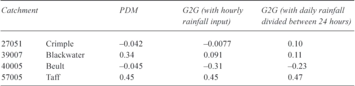
Table 4. R2
performance statistics using ERA-driven RCM rainfall.
Catchment PDM G2G (with hourly G2G (with daily rainfall rainfall input) divided between 24 hours)
27051 Crimple 0.042 0.0077 0.10
39007 Blackwater 0.34 0.091 0.11
40005 Beult 0.045 0.31 0.23
57005 Taff 0.45 0.45 0.47
3s
Ŧ
1
Flow [m
s
Ŧ
1]
Flow [m
3
Hourly flow
Daily flow (a)
42000 42720 43440 44160 44880 45600
Ŧ10 10 30 50 70 90
]
1750 1780 1810 1840 1870 1900
Ŧ20 0 20 40 60 80
Time(days) Time(hours)
Daily flow Hourly flow (b)
240000 26160 28320
10 20 30 40 50 60 70 80
Flow [m
3s
Ŧ
1]
1000 1090 1180
0 10 20 30 40 50 60 70
Flow [m
3s
Ŧ
1]
Time(hours)
Time(days)
Hourly flow
Daily flow (c)
154800 17640 19800
200 400
Flow [m
3s
Ŧ
1]
645 735 825
0 100 200
Flow [m
3s
Ŧ
1]
Time(hours)
Time(days)
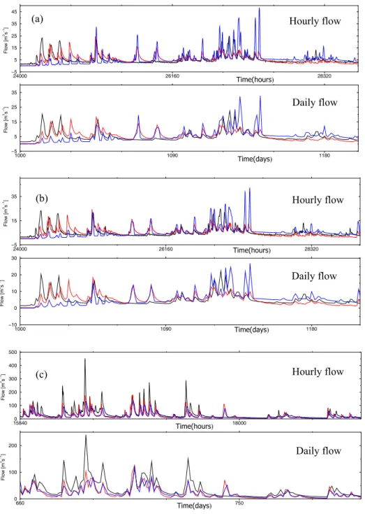
545 occasionally improves on the PDM in terms of the R2
criterion when daily rainfalls are spread into hourly time-steps. However, any modest improvement may be an artefact of the smoothing process arising from the daily averaging of both the rainfall input and the flow output and should, therefore, be treated with caution. The conversion from hourly to ESD rainfall has led to an improvement in G2G model performance. Calibration of the G2G routing model using daily rainfall data is likely to have led to a smoother
model simulation that is unable to get the peak flow or timing correct when examined at a smaller time-step. Figure 10 (a) and (b) shows the hourly and daily average flow series obtained for the Blackwater. In Fig. 10 (b), the hourly rainfall data have been replaced by daily rainfall divided equally between the 24 hourly time-steps. Daily average flows are usually significantly lower than hourly flows as sharp peak flows averaged across 24 hours result in reduced peaks.
24000 26160 28320
Ŧ5 5 15 25 35 45
Flow [m
3s
Ŧ
1]
1000 1090 1180
Ŧ5 5 15 25 35
Flow [m
3s
Ŧ
1]
Time(hours)
Time(days)
(a) Hourly flow
Daily flow
24000 26160 28320
Ŧ5 15 35
Flow [m
3s
Ŧ
1]
1000 1090 1180
Ŧ10 0 10 20 30
Flow [m
3s
Ŧ
1]
Time(hours)
Time(days)
(b)
Daily flow Hourly flow
158400 18000
100 200 300 400 500
Flow [m
3s
Ŧ
1]
660 750
0 100 200
Flow [m
3s
Ŧ
1]
Time(hours)
Time(days)
(c) Hourly flow
Daily flow
546
FLOOD FREQUENCY CURVE ASSESSMENT
The relationship between flood magnitude and rarity can be described by the flood frequency curve derived from a time-series of river flows at a particular location. The flood frequency curve shows flow rates at different return periods, which provide a measure of how often a flood of a given magnitude is likely to be equalled or exceeded. This section compares the performance of the two models (parameter-generalised PDM and G2G) in terms of flood frequency estimation, through the derivation of flood frequency curves from the flow time-series. In this case, a peaks-over-threshold (POT) method is applied (Naden, 1992) as described in Kay et al. (2006). A POT series is preferred over an annual maximum (AM) series here because it is generally considered to be more robust, particularly given the short period of overlap between the available raingauge and flow data and the period of the ERA-driven RCM data (~9 years). The result is a flood frequency curve which relates peak flow to return period continuously. It is important to note that, although a statistical distribution is fitted to the point data, this curve is not intended to be extrapolated to higher return periods. It simply interpolates between point data, and smoothes the effect of jumps in sampled peak flow values. It is the fitted curves which will be analysed when results are compared.
For the four catchments for which the G2G has been calibrated (Crimple, Blackwater, Beult and Taff), flood frequency curves for the G2G have been compared with (i) results for the parameter-generalised PDM using hourly raingauge data and (ii) curves derived using hourly flow measurements. Flood frequency curves were analysed at a daily time-step although curves have also been derived at an hourly time-step. Comparing the two models at a daily time-step tends to favour the G2G model as it has been calibrated using only daily observations of flow and rainfall. The difference in resolution of rainfall data, and the time-step of model calibration for the two models, makes an equitable comparison impossible.
Flood frequency curves, derived for daily average flows from the parameter-generalised PDM and the G2G, are shown in Fig. 11 for the four catchments for which the G2G has been calibrated. Flood frequency curves derived from actual flow observations are also shown. Overall, hourly flood frequency curves (not shown here) obtained from flows estimated by the G2G model tend to underestimate peak flow for a given return period. Daily frequency curves from the G2G model are closer to observed daily flood frequency curves as shown in Fig. 11. This may reflect the fact that the G2G model is adjusted for use with daily rainfall data and has been calibrated with reference to daily flow measurements; it is also harder to model variation in flows
0.1 1 10 100
0.5 1 1.5 2 2.5
Daily peak flow [m
3 s
Ŧ
1 ]
0.1 1 10 100
0 10 20 30 40
Daily peak flow [m
3s
Ŧ
1]
0.1 1 10 100
Ŧ50 0 50 100 150
Daily peak flow [m
3s
Ŧ
1]
0.1 1 10 100
Return period [years] 0
100 200 300 400
Daily peak flow [m
3 s
Ŧ
1 ]
(d)
(c)
(b)
(a)
at a smaller time-step.
For all but the Beult catchment (Fig. 11c), the parameter-generalised PDM and G2G daily flood frequency curves are very similar. The larger peak flows modelled by the G2G at higher return periods for the Beult are likely to be a result of poor simulation of baseflow, leading to excessive surface flows following heavy rainfall. Underestimation of modelled peak flows for the Taff catchment in South Wales for both models is less easy to diagnose. The Taff is a steep, highly responsive catchment with a minimal baseflow contribution, so little of the rainfall entering the catchment will be stored for long periods. Kay et al. (2006) compared the flood frequency curve for this catchment using both RCM rainfall and observations as input to the parameter-generalised PDM. The Taff was one of only two catchments out of 15 for which flood frequency estimates gave poor visual correspondence with those derived using observed rainfall and PE data. RCM-derived annual average rainfall for the Taff was underestimated by nearly 40% when compared with rainfall observations. The causes for this are still being investigated, although an apparent amplification of the rain-shadow effect by the RCM (Frei et al., 2003) may be implicated.
Conclusions
A simple modelling framework has been developed to translate regional climate model estimates of rainfall (and potential evaporation) into estimated river flow at a daily or sub-daily time-step. The scheme can provide regional, area-wide estimates of future changes in river flow at a daily or (with less accuracy) a sub-daily time-step. Its simple grid-based configuration allows it to be coupled directly to climate models, land-surface schemes and ocean models for studies of the effects of climate change on small to medium catchments (from a UK perspective), as well as for studies into dependencies between sea-surges and extreme river flows.
The G2G model presented here routes gridded runoff estimates to estimate river flows which can be compared with gauged measurements. The routing component uses a kinematic wave scheme which can also be expressed as a cascade of linear reservoirs. Model results for contrasting catchments across the UK are encouraging and indicate circumstances under which the G2G model performs well or less well. The parameter-generalised PDM catchment-based model provides an additional means of assessing model performance, by setting a standard against which the G2G may be compared. It also provides an additional set of estimates of catchment hydrological response.
To address a range of scientific issues, two different sources of precipitation were used as input to the G2G model:
(i) 5 km grid daily rainfall interpolated from raingauge data (1958 to 2002).
(ii) 25 km grid hourly precipitation from a regional climate model (RCM) driven by re-analysis (ERA) data (1979 to 1993).
The first, an observation-based estimate of spatial rainfall, is most useful for G2G model development, calibration and assessment. RCM model-based rainfall provides a basis for impact assessment under different climates using the G2G hydrological model: its success in simulating flows over the recent past serves to add confidence to its application under future climate scenarios.
For the model simulations that use hourly RCM precipitation data, corresponding RCM estimates for temperature, humidity, wind speed and net radiation have been used to derive daily PE. The procedure for calculating PE from RCM estimates is as close as possible to that used to derive MORECS PE. For model simulations involving the 5 km daily rainfall, monthly 40 km MORECS PE has been used.
The results of using these sets of input data are as follows.
1. Use of the best available data (5 km daily rainfall and daily flow observations) to assess the G2G model performance indicates that the model performs best on catchments the hydrological response of which is topographically-driven, rather than baseflow/soil dominated. The median value of the R2 performance
criterion for baseflow-dominated catchments is 0.22, whilst for catchments dominated by surface flow it is 0.64.
2. For four catchments where the G2G is compared informally with the parameter-generalised PDM using observation-based rainfall as input, the G2G performs reasonably well when calibrated to each catchment, although the performance of the parameter-generalised PDM is better for all catchments.
3. The difference between the performance of the G2G and the generalised PDM is reduced when ERA-driven hourly RCM rainfall data are used as input to both models, particularly when assessed at a daily time-step. The R2 values from the parameter-generalised PDM and
G2G are generally comparable but there are some differences.
of daily average flows to construct the flood frequency curve tends to produce closer agreement between model- and observation-derived curves. This may be due to the daily time-step of the data being used to adjust the G2G to catchment conditions. The model has not been adjusted to simulate the hourly flood hydrograph and its peaks and an assessment at this time-step might be expected to expose errors.
An important modelling challenge is to find a physical-conceptual way of linking the small number of regional parameters of the G2G model to datasets that reflect any significant influences of topography, land cover, soil and geology (for which digital spatial datasets are available). The form of PDM used here is a prototype empirical parameter-generalisation based on catchment-integrated properties derived from such datasets. Ongoing research (for example, Calver et al., 2005) is attempting to improve the basis of this parameter-generalisation. The prototype G2G model outlined here has employed physical-conceptual ways of using topographic data to support model configuration of the flow routing component and to invoke terrain-slope control of runoff production. Further work aims to embrace consideration of soil properties, land-cover and geology. The focus here has been on G2G flow routing under the dominant control of topography as represented by a digital terrain model. Coupling with a more comprehensive runoff production (land-surface) scheme incorporating topographic, soil and geology controls on water movement and storage is being researched. There is clearly significant scope for trialling different formulations of both the routing and runoff production components of the G2G model, capitalising on the availability of hydrologically-relevant digital datasets.
Improving understanding of the potential impacts of flooding arising from climate change is an important scientific objective worldwide. The outputs of regional climate models run under current and future emissions scenarios are increasingly valuable in flood impact studies. It is imperative that advances continue to be made on physical-conceptual modelling of water flow movement and storage on an area-wide basis in support of flood impact studies and for coupling to climate and ocean models. This will ensure outcomes that are plausible for guiding policy on coping with climate change and its impact on the water flow regime and the wider environment and society it influences.
Acknowledgements
This work was funded by the Department for Environment, Food and Rural Affairs (Defra) Climate Prediction Programme (PECD 7/12/37) and the Met Support Group of the Ministry of Defence via the Met Office. Observations of river flow were provided by the Environment Agency via the National River Flow Archive (NRFA) at CEH Wallingford. The authors would particularly like to thank Felicity Sanderson and Terry Marsh at the NRFA for help and advice concerning these data.
References
Aroro, V.K. and Boer, G.J., 1999. A variable velocity flow routing algorithm for GCMs. J. Geophys. Res.,104, D24, 3096530979. Bell, V.A. and Moore, R.J., 1998. A grid-based distributed flood forecasting model for use with weather radar data: Part 1: Formulation. Hydrol. Earth Syst. Sci., 2, 265281.
Calver, A., Crooks, S.C., Jones, D.A., Kay A.L., Kjeldsen, T.R. and Reynard, N.S., 2005. National river catchment flood frequency method using continuous simulation. Report to the UK Department for Environment, Food and Rural Affairs, Technical Report FD2106/TR and Project Record FD2106/PR, CEH Wallingford, UK. 135pp plus 141pp (appendices). Calver, A., Lamb, R., Kay, A.L. and Crewett, J., 2001. The
continuous simulation method for river flood frequency estimation. Department for Environment, Food and Rural Affairs Project FD0404 Final Report, CEH Wallingford, UK. 56pp + appendices.
Crewett, J., Lamb, R. and Calver, A., 1999. Spatial generalisation of model parameters for flood frequency estimation using continuous simulation: Recent research advances. Report for MAFF Project FD0404, Institute of Hydrology, Wallingford, UK. 18pp.
Ducharne, A., Golaz, C., Leblois, E., Laval, K., Polcher, J., Ledoux, E. and de Marsily, G., 2003. Development of a high resolution runoff routing model: calibration and application to assess runoff from the LMD GCM. J. Hydrol., 280, 207228. Fekete, B.M., Vorosmarty, C.J. and Lammers, R.B., 2001. Scaling
gridded river networks for macroscale hydrology: development, analysis and control of error. Water Resour. Res.,37, 1955 1967.
Fowler, H.J., Ekström, M., Kilsby, C.G. and Jones, P.D., 2005. New estimates of future changes in extreme rainfall across the UK using regional climate model integrations. 1: assessment of control climate. J. Hydrol., 300, 212233.
Frei, C., Christensen, J.H., Deque, M., Jacob, D., Jones, R.G. and Vidale, P.L., 2003. Daily precipitation statistics in Regional Climate Models: evaluation and intercomparison for the European Alps. J. Geophys. Res., 108, D3, 4124.
Giorgi, F., Hewitson, B.C., Christensen, J., Hulme, M., Von Storch, H., Whetton, P., Jones, R., Mearns, L. and Fu, C., 2001. Regional Climate Information - Evaluation and Projections. In: Climate Change 2001: The Scientific Basis, Houghton et al. (Eds.), Cambridge University Press, Cambridge, UK, 583638. Hagemann, S. and Dumenil, L., 1998. A parameterisation of the
lateral water flow for the global scale. Clim. Dynam.,14, 17 31.
Hulme, M., Jenkins, G.J., Lu, X., Turnpenny, J.R., Mitchell, T.D.,
Jones, R.G., Lowe, J., Murphy, J.M., Hassell, D., Boorman, P., McDonald, R. and Hill, S., 2002. Climate change scenarios for the UK: UKCIP02 scientific report, Tyndall Centre, Norwich, UK. 112pp.
Huntingford, C., Jones, R.G., Prudhomme, C., Lamb, R., Gash, J.H.C. and Jones, D.A., 2003. Regional climate-model predictions of extreme rainfall for a changing climate. Quart. J. Roy. Meteorol. Soc, 129, 16071621.
Institute of Hydrology, 1980. Low River Flows in the United Kingdom, Institute of Hydrology Report No. 108. Wallingford, UK. 88pp + appendices.
Jones, D.A. and Moore, R.J., 1980. A simple channel flow routing model for real-time use. IAHS Publication no. 129, 397408. Kay, A.L., 2003. Estimation of UK flood frequencies using RCM
rainfall: A further investigation. Report to the Department for Environment, Food and Rural Affairs, Hadley Centre Annex 15a, CEH Wallingford, UK. 48pp.
Kay, A.L., Reynard, N.S. and Jones, R.G., 2006. RCM rainfall for UK flood frequency estimation. I. Method and validation. J. Hydrol., 318, 151162.
Kay, A.L., Bell, V.A., Moore, R.J. and Jones, R.G., 2003. Estimation of UK flood frequencies using RCM rainfall: An initial investigation. Report to the Department for Environment, Food and Rural Affairs, Hadley Centre Annex 15a, CEH Wallingford, UK. 40pp.
Lamb, R., 1999. Calibration of a conceptual rainfall-runoff model for flood frequency estimation by continuous simulation. Water Resour. Res., 35, 31033114.
Lamb, R., Crewett, J. and Calver, A., 2000. Relating hydrological model parameters and catchment properties to estimate flood frequencies from simulated river flows. British Hydrological Society 7th National Hydrology Symposium, University of Newcastle, UK. 3.573.64.
Leopold, L.B., Wolman, M.G. and Miller, J.P., 1978. Fluvial Processes in Geomorphology. W.H. Freeman, San Francisco, USA. 818pp.
Lucas-Picher, P., Arora, V.K., Caya, D. and Laprise, R., 2003. Implementation of a large-scale variable velocity flow routing algorithm in the Canadian Regional Climate Model (CRCM). Atmos.-Ocean, 41, 139153.
Jain, M.K. and Singh, V.P., 2005. DEM-based modelling of surface runoff using diffusion wave equation. J. Hydrol., 302, 107126. Jones, D.A. and Moore, R.J., 1980. A simple channel flow routing model for real-time use. IAHS Publication no. 129, 397408. Miller, J.R., Russell, G.L. and Caliri, G., 1994. Continental scale
river flow in climate models. J. Climate, 7, 914928.
Moore, R.J., 1985. The probability-distributed principle and runoff production at point and basin scales. Hydrolog. Sci. J., 30, 273 297.
Moore, R.J., 1999. Real-time flood forecasting systems: perspectives and prospects. Chapter 11. In: Floods and landslides: Integrated Risk Assessment, R. Casale and C. Margottini (Eds.), Springer, Berlin, Germany. 147189. Moore, R.J. and Jones, D.A., 1978. An adaptive finite-difference
approach to real-time channel flow routing. In: Modelling, Identification and Control in Environmental Systems, G.C.Vansteenkiste(Ed.), North-Holland, Amsterdam, The Netherlands. 153170.
Monteith, J.L., 1965. Evaporation and environment. Symposia of the Society for Experimental Biology, 19, 205234.
Naden, P.S., 1992. Analysis and use of peaks-over-threshold data in flood estimation.In: Floods and Flood Management, A.J. Saul, (Ed.), Kluwer, Dordrecht, The Netherlands. 131143. Oki, T., Agata, Y., Kanae, S., Saruhashi, T., Yang, D. and Musiake,
K., 2001. Global assessment of current water resources using total runoff integrating pathways. Hydrolog. Sci. J., 46, 983996. Olivera F. and Raina, R., 2003. Development of large scale gridded river networks from vector stream data. J. Amer. Water Resour. Assoc., October, 12351248.
Sausen, R., Schubert, S. and Dumenil, L., 1994. A model of river-runoff for use in coupled atmosphere-ocean models. J. Hydrol.,
155, 337352.
Shuttleworth, W.J., 1993. Evaporation. In: Handbook of Hydrology, D.R.Maidment (Ed.), McGraw Hill, New York, USA. 4.14.53. Singh, V.P., 1996. Kinematic wave modelling in water resources:
Surface water hydrology. Wiley, New York, USA. 1399pp. Thompson, N., Barrie, I.A. and Ayles, M., 1982. The
Meteorological Office Rainfall and Evaporation Calculation System: MORECS(July 1981). Hydrological Memorandum No. 45, Met Office, Bracknell, UK. 69pp.
U.S. Geological Survey, 1998. HYDRO 1K: Elevation derivative database, http://edcwww.cr.usgs.gov/landdaac/gtopo30/hydro/ index.html, USGS EROS data Centre, Sioux Falls, South Dakota, USA.