Carbon fixation prediction during a bloom of <i>Emiliania huxleyi</i> is highly sensitive to the assumed regulation mechanism

(1)

BGD

6, 5339–5372, 2009

Prediction ofE. hux

carbon fixation

O. Bernard et al.

Title Page

Abstract Introduction

Conclusions References

Tables Figures

◭ ◮

Back Close

Full Screen / Esc

Printer-friendly Version

Interactive Discussion Biogeosciences Discuss., 6, 5339–5372, 2009

www.biogeosciences-discuss.net/6/5339/2009/ © Author(s) 2009. This work is distributed under the Creative Commons Attribution 3.0 License.

Biogeosciences Discussions

Biogeosciences Discussionsis the access reviewed discussion forum ofBiogeosciences

Carbon fixation prediction during a bloom

of

Emiliania huxleyi

is highly sensitive to

the assumed regulation mechanism

O. Bernard1,2, A. Sciandra2, and S. Rabouille2

1

COMORE-INRIA, BP 93, 06902 Sophia-Antipolis Cedex, France

2

LOV, UMR 7093, Station Zoologique, BP 28, 06234, Villefranche-sur-mer, France Received: 1 April 2009 – Accepted: 5 May 2009 – Published: 28 May 2009 Correspondence to: O. Bernard (olivier.bernard@inria.fr)

(2)

BGD

6, 5339–5372, 2009

carbon fixation

O. Bernard et al.

Title Page

Tables Figures

◭ ◮

Back Close

Full Screen / Esc

Interactive Discussion Abstract

Large scale precipitation of calcium carbonate in the oceans by coccolithophorids plays an important role in carbon sequestration. However, there is a controversy on the ef-fect of an increase in atmospheric CO₂ concentration on both calcification and photo-synthesis of coccolithophorids. Indeed recent experiments, performed under nitrogen

5

limitation, revealed that the associated fluxes may be slowed down, while other authors claim the reverse. We designed models to account for various scenarii of calcification and photosynthesis regulation in chemostat cultures ofEmiliania huxleyi, based on dif-ferent hypotheses on the regulation mechanism. These models consider that either carbon dioxide, bicarbonate, carbonate or calcite saturation state (Ω) is the regulating

10

factor. All were calibrated to predict the same carbon fixation rate in nowadayspCO₂, but they turn out to respond differently to an increase in CO2 concentration. Thus, using the four possible models, we simulated a large bloom of Emiliania huxleyi. It results that models assuming a regulation by CO2₃− orΩ predicted much higher car-bon fluxes. The response when considering a doubledpCO2was different and models

15

controlled by CO2or HCO −

3 led to increased carbon fluxes. In addition, the variability between the various scenarii proved to be in the same order of magnitude than the response topCO2increase. These sharp discrepancies reveal the consequences of model assumptions on the simulation outcome.

1 Introduction

20

Coccolithophorids play an important role in CO2trapping (Frankignoulle et al., 1994), since they transform dissolved inorganic carbon (DIC) into respectively particulate or-ganic and inoror-ganic matter which, being denser than seawater, sink towards the ocean floor. Such export of both particulate organic carbon (POC) (see Eq. 1) and particulate inorganic carbon (PIC) (see Eq. 2), operated by the biological pump from the

sur-25

(3)

BGD

6, 5339–5372, 2009

carbon fixation

O. Bernard et al.

Title Page

Tables Figures

◭ ◮

Back Close

Full Screen / Esc

Interactive Discussion (Klepper et al., 1994; Falkowski, 1997).

6CO₂+12H₂O−→C₆H₁₂O₆+6O₂+6 H₂O (1)

Ca2++2HCO−₃−→CaCO3+CO2+H2O (2)

Coccoliths formation thus accounts for nearly 70% of the biogenic carbonate precipi-tation in the oceans (Houghton et al., 1996). Yet, such structures are relatively sensitive

5

to pH and tend to dissolve when the water becomes too acidic. It is expected that a doubling inpCO2 will have direct consequences on the ability of these organisms to maintain their growth rate (Riebesell et al., 2000; Sciandra et al., 2003). As a corollary, acidification of the oceans due to increase in atmosphericpCO₂(Orr et al., 2005) could jeopardize their role as a CO2pump.

10

Hence, how coccolithophorids may respond to shifts in globalpCO2is a critical ques-tion to be answered. However, if the chemical phenomena driving the coccoliths dis-solution are well known, the effects of pCO2 changes, whether on photosynthesis or on calcification, are still subject to intense debates (Paasche, 2002; Berry et al., 2002; Riebesell et al., 2008). Contradictory observations were made in batch experiments,

15

where doublingpCO2 either led to a decrease (Riebesell et al., 2000) or an increase (Iglesias-Rodriguez et al., 2008) in calcification inEmiliana huxleyi while photosyn-thesis was enhanced. Continuous cultures experiments in chemostats supported the hypothesis that both photosynthesis and calcification decrease (Sciandra et al., 2003), while photosynthesis was increased in a study with non calcifying strain (Leonardos

20

and Geider, 2005).

Since the pioneer works of Paasche (1968) the functional relationship between cal-cification and photosynthesis continues to cause intense research leading to contra-dictory results for several reasons (see Paasche, 2002, for a compilation). The nature of the physiological coupling between photosynthesis and calcification is far from being

25

(4)

BGD

6, 5339–5372, 2009

carbon fixation

O. Bernard et al.

Title Page

Tables Figures

◭ ◮

Back Close

Full Screen / Esc

Interactive Discussion On the other hand, several experiments have shown that photosynthesis can directly

or indirectly use the CO2 produced by calcification; this is an advantage forE. huxleyi whose affinity for dissolved CO2in seawater is low (Buitenhuis et al., 1999). Thirdly, the kind of transport (active vs. passive) and the C substrates (CO₂vs. HCO−₃-) implied in the uptake of DIC are still subject to debate. It is only recently that carbon concentration

5

mechanisms (CCM), implying intra or extracellular carbonic anhydrase enzymes, were detected inE. huxleyi (Nimer and Merrett, 1996). Nevertheless the CCM efficiency in E. huxleyiseems low compared to others species (Rost et al., 2003, 2006).

Considering the chemical equations for photosynthesis (1) and calcification (2), a classical Michaelis-Menten based kinetics for growth could be proposed, involving,

re-10

spectively CO₂ and HCO−₃. However, such representation follows the dogmatic as-sumption that photosynthesis is regulated by the CO2 concentration only, and calcifi-cation is regulated by HCO−₃only. Yet, Riebesell et al. (2000) and Sciandra et al. (2003) indirectly demonstrated that HCO−₃ could not regulate calcification: their experiments showed that an increase in HCO−₃led to a decrease in the calcification rate. These

con-15

tradictory experimental results spurred Bernard et al. (2008) to propose and analyse 12 models based on different assumptions as for the inorganic carbon species regulating calcification and photosynthesis, taken among CO2, HCO

−

3 and CO 2−

3 . Model simula-tions suggested that only the models where carbonate ion regulates calcification could reproduce the decrease in calcification rate after apCO₂doubling, hence refuting the

20

general assumption of a regulation by HCO−₃. Indeed, CO2₃−is the only species whose concentration decreases when pCO2 increases. This hypothesis is corroborated by Merico et al. (2006) who suggest that the condition of high CO2₃− can be considered as a crucial ecological factor for the success ofE. huxleyi. However, this hypothesis needs clarification from a biological point of view. As stated by Riebesell (2004), carbonate

25

(5)

BGD

6, 5339–5372, 2009

carbon fixation

O. Bernard et al.

Title Page

Tables Figures

◭ ◮

Back Close

Full Screen / Esc

Interactive Discussion model, based on the representation of a cell quota, is a Droop-like model (Droop, 1968;

Burmaster, 1979; Droop, 1983) in which we added the dependence to both inorganic carbon and light.

Our goal is to point out how the generic model of (Bernard et al., 2008), successively run with the different regulating factors, can predict significantly different amounts and

5

fluxes of carbon. We simulated the typical situation of anEmiliania huxleyilate-Spring bloom, following a diatoms bloom which depleted the inorganic carbon stock (Riebesell et al., 1993). The four versions of the model only differ by their assumption on the factor regulating the inorganic carbon uptake. In this simplified model, we assume that all the chemical and biological concentrations are homogeneous in the mixed layer. The main

10

idea developed throughout this paper is that some transient phenomena can lead to paradoxical effects on the predicted carbon fluxes. Hence we show that, depending on the supposed regulating factor, the exported carbon can vary two-fold. Results also reveal that the fluxes variability, due to the assumed regulating factor, is higher than the influence of apCO2increase, because of the slow transfer rate of inorganic carbon

15

through the atmosphere – seawater interface.

In the following section, we present the biological model of growth and calcification and describe its variants, according to the chemical species regulating the inorganic carbon compartment. We then recall classical modelling theories of the carbonate sys-tem dynamics in seawater. The hydrodynamical structure of the water column, in the

20

(6)

BGD

6, 5339–5372, 2009

carbon fixation

O. Bernard et al.

Title Page

Tables Figures

◭ ◮

Back Close

Full Screen / Esc

Interactive Discussion 2 Modelling growth and calcification of coccolithophorids

2.1 Phytoplankton growth in conditions of nitrogen limitation

Uptake of inorganic nitrogen (nitrate, denoted S₁) by the phytoplanktonic biomass (whose particulate nitrogen concentration is denoted N), can be represented by the following mass flow, whereρ(.) is the nitrate absorption rate:

5

S1

ρ(.)X

−→N (3)

The flux of inorganic carbon into organic biomass X and coccoliths C is associated to a flux of calcium (Ca2+, denoted S2) and of dissolved inorganic carbon (D), where

µ(.) is the photosynthesis rate:

1−α

α S2+α1D

µ(.)X

−→ 1−_ααC+X (4)

10

Here, for sake of simplicity, we assume that photosynthesis and calcification are coupled (see Bernard et al., 2008, for models where these processes are uncoupled). The constantα represents the proportion of the total up taken DIC which is allocated to photosynthesis.

The next step in the model development is the mathematical expression for both the

15

nitrate absorption rateρ(.) and the photosynthesis rateµ.

Generally, nitrate uptake is assumed to depend on external nitrate concentration NO₃, following a Michaelis-Menten type equation (Dugdale, 1967):

ρ(S₁)=ρmS1/(S1+kN) (5)

The expression of the rate of inorganic carbon acquisition is more tricky; as shown

20

(7)

BGD

6, 5339–5372, 2009

carbon fixation

O. Bernard et al.

Title Page

Tables Figures

◭ ◮

Back Close

Full Screen / Esc

Interactive Discussion photosynthesis while HCO−₃would be the substrate for calcification. Therefore the

reg-ulation of growth and calcification could theoretically be triggered by CO₂or HCO−₃. In addition, we examined the possibility that CO2₃−is involved in the regulation of inorganic carbon acquisition, as suggested by recent works (Bernard et al., 2008). Last, we also consider that availability of calcium can potentially regulate photosynthesis and

calci-5

fication. In this last hypothesis, µ(.) is a function ofΩ, the saturation state of calcite (CaCO3):

Ω=[Ca

2+_][CO2− 3 ]

Ksp

(6)

where the solubility constant yieldsK_sp=5.15 10−7mol2L−2.

As a consequence, in the sequel we examine four possible models that only differ by

10

the regulation mechanism of inorganic carbon acquisition:

– CO2is the regulating species, and thusµ(Q,CO2) is an increasing function of both Q and CO₂.

– HCO−₃is the regulating species, and thusµ(Q,HCO−₃) is an increasing function of both Q and HCO−₃.

15

– CO2₃− is the regulating species, and thusµ(Q,CO2₃−) is an increasing function of both Q and CO2₃−.

– Ωis the regulating species, and thusµ(Q,Ω) is an increasing function of both Q andΩ.

To keep a general denomination, we denoteµ_p(Q,D_p) the growth rate, where,

de-20

pending on the modelM_p,Dpis chosen among CO2, HCO − 3, CO

2−

(8)

BGD

6, 5339–5372, 2009

carbon fixation

O. Bernard et al.

Title Page

Tables Figures

◭ ◮

Back Close

Full Screen / Esc

Interactive Discussion The analytical expression of µp(Q,Dp) is then based on the Droop model (Droop,

1968, 1983):

µ(Q, D_p)=µ¯¯(I0)(1−

kQ

Q)

D_p Dp+kD_p

−R (7)

wherek_Qandk_D_p are, respectively the subsistence quota and the half-saturation con-stant for the chosen regulating species. The mortality rateR accounts for respiration

5

and grazing losses, and is supposed constant. The maximum hypothetical growth rate at lightIis denoted ¯µ(I), and we use the following expression, supported e.g. by Nimer and Merrett (1993):

¯

µ(I)=µ¯ I

I+KI

(8)

The maximum hypothetical growth rate averaged on the mixed layer is denoted ¯¯µ(I0).

10

It depends on the incident irradianceI0.

To compute this term, we take into account the exponential decrease of light with depth. We use the model of Oguz and Merico (2006) assuming that light extinction rate is the sum of a constant ratek1 (due to the background and suspended material extinction) and of a rate proportional to phytoplanktonic nitrogen N (due to the

biomass-15

specific extinction of the phytoplankton).

I(z)=I0 exp(−(k1+k2N)z) (9)

The average value of the maximum hypothetical growth rate ¯µ_I_(z)I(z)₊_K

I in the mixed layer of depth L, can then be computed as follows:

¯¯

µ(I₀)=1

L ZL

0 ¯

µ I0exp(−(k1+k2N)z) I0exp(−(k1+k2N)z)+KI

dz (10)

(9)

BGD

6, 5339–5372, 2009

carbon fixation

O. Bernard et al.

Title Page

Tables Figures

◭ ◮

Back Close

Full Screen / Esc

Interactive Discussion a straightforward computation leads to:

¯¯

µ(I0)= 1 (k1+k2N)L

ln I0+KI

I0exp(−(k1+k2N)L)+KI

(11)

2.2 Inorganic carbon modelling

In order to compute CO2, HCO − 3, CO

2−

3 and Ωfrom DIC (D) and Ca 2+ _(S

2), classical equations of the seawater carbonate system must be considered (Zeebe and

Wolf-5

Gladrow, 2003; Millero, 2007).

The carbonate alkalinity (CA) represents the sum of the electric charges carried in the carbonate system:

CA=[HCO−₃]+2[CO2₃−] (12)

The total alkalinity (TA) is defined by (see Zeebe and Wolf-Gladrow, 2003, for more

10

details):

TA=CA+[B(OH)−₄]+[OH−]−[H+] (13)

We denote λ=TA−2[Ca2+]=TA−2S2. To a first approximation, the ions that most contribute toλdepend on the salinity and remain constant.

Following the previous considerations, carbonate alkalinity then only depends on

15

calcium: CA=λ−λ0+2S2 (where, to a first approximation, λ0=[B(OH) − 4]+[OH

− ]−[H+] remains constant compared to CA). In order to compute [HCO−₃] and [CO2₃−], we use the dissociation constants of the carbon dioxide (K1) and bicarbonate (K2):

K1=

h[HCO−₃] [CO2]

andK2=

h[CO2₃−]

(10)

BGD

6, 5339–5372, 2009

carbon fixation

O. Bernard et al.

Title Page

Tables Figures

◭ ◮

Back Close

Full Screen / Esc

Interactive Discussion where h is the proton concentration, [H+].The total dissolved inorganic carbon (D) is

defined as:

D=[HCO−₃]+[CO₃2−]+[CO2] (15)

Note that, in the considered pH range, [HCO−₃]>>[CO2₃−]>>[CO2] (see for example Zeebe and Wolf-Gladrow, 2003). It follows that bicarbonate is the main carbon species

5

in the carbonate system:

[HCO−₃]≃D (16)

and that the carbonates concentration can be deduced from Eqs. (12) and (15):

[CO2₃−]≃CA−D (17)

With this approximation, we can now compute the following ratio:

10

r=_[CAD , using Eqs. (12), (15), and (14);r reads:

r=h+K2+h

2

/K1 h+2K2

(18)

It follows that h can be computed as a function ofr:

h=u(r)=

−1+r+

q

(1−2r)(1−4K2/K1)+r2 _K

1

2 (19)

Now using Eqs. (14) and (12), we can compute the CO₂concentration:

15

[CO₂]=CA

K1 h2 h+2K2

=CAv(r)=ψ(S₂,D) (20)

(11)

BGD

6, 5339–5372, 2009

carbon fixation

O. Bernard et al.

Title Page

Tables Figures

◭ ◮

Back Close

Full Screen / Esc

Interactive Discussion so resolves the exact concentration of the chemical species. The used Matlab code

is a supplement to Zeebe and Wolf-Gladrow (2003), modified to account for calcium consumption.

When coupling growth, calcification and inorganic carbon models, we get the models proposed in Bernard et al. (2008) (plus the model where calcite saturation state is the

5

regulating factor). The analysis in Bernard et al. (2008) demonstrated thatM_pmodels whereDp was either CO2 or HCO

−

3supported the results of Iglesias-Rodriguez et al. (2008), while models where CO2₃− orΩwas the regulating factor supported the results obtained by Sciandra et al. (2003). To get a qualitative prediction of the experimen-tal results reported by Riebesell et al. (2000), calcification and photosynthesis had to

10

be decoupled, with photosynthesis driven by CO2 or HCO −

3and calcification driven by CO2₃−orΩ.

3 Modelling a bloom ofE. huxleyi in a mixed layer

3.1 Considered simplified physics

In summer, density gradients generated by increasing temperatures lead to water

strat-15

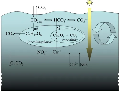
ification. The surface layer remains mixed over a generally shallow depth. Here we considered a mixed layer depth L of 15 m, and to keep the model as simple as possible we assumed, as in Tyrell and Taylor (1996), an homogeneous distribution. We simu-lated the growth of coccolithophorids in this mixed layer, as represented in Fig. 1. CO2 concentration in the water equilibrates with that in the atmosphere, following the diff

er-20

ence in concentration between the two compartments and according to the diffusion coefficientKL.

In the water, CO2equilibrates with HCO −

3and CO 2−

3 . The CO2pool in the water is also affected by the coccolithophorids activity, being fueled by respiration and consumed through the processes of photosynthesis and calcification (see Eq. 4). The model

(12)

BGD

6, 5339–5372, 2009

carbon fixation

O. Bernard et al.

Title Page

Tables Figures

◭ ◮

Back Close

Full Screen / Esc

Interactive Discussion simulates a nitrate uptake limited by the availability of NO₃ , as illustrated by Eq. (3).

NO3, DIC and Ca

2+ _{in the mixed water are replenished from the deeper waters (with}

an exchange rateK_d) whose concentration are, respectively, S1,0, S2,0and D0. As the water acidity affects the coccoliths persistence, we accounted for a possible dissolution of coccoliths whose rate is dependent upon pH through the calcite saturation state. We

5

assume that this rate can be written as Kdiss

Ω , where Kdiss is the dissolution rate when

Ω=1. Settlement of calcite (coccoliths) is represented through CaCO3 sinking below the mixed layer.

3.2 Model equations

Model equations can then be directly deduced from the mass flows (3) and (4). Dp

10

is the regulating factor (among CO2, HCO − 3, CO

2−

3 and Ω) assumed to control both photosynthesis and calcification. The system of equations reads:

˙

S₁=Kd(S1,0−S1)−ρ(S1)X (21)

˙

Q=ρ(S1)−µ(Q, Dp)Q (22)

˙

X=−KdX+µ(Q, Dp)X−RX−KsedX (23)

15

˙

C=−KdC+

1−α

α µ(Q, Dp)X−KsedC− Kdiss

Ω C (24)

˙

D=K_d(D0−D)− 1

αµ(Q, Dp)X+RX (25)

−K_L(ψ(S2,D)−KHpCO2)+

Kdiss

Ω C (26)

˙

S₂=Kd(S2,0−S2)− 1−α

(13)

BGD

6, 5339–5372, 2009

carbon fixation

O. Bernard et al.

Title Page

Tables Figures

◭ ◮

Back Close

Full Screen / Esc

Interactive Discussion WhereK_d is the exchange rate through the thermocline andKsed the sedimentation

rate.

The initial conditions have been chosen assuming that coccolithophorids bloom right after a large diatom bloom which reduced the nitrate and inorganic carbon concentra-tions in the mixed layer (Riebesell et al., 1993). Inspired by the pCO₂ observations

5

during bloom experiments (Keeling et al., 1996; Benthien et al., 2007), we assume that 0.2 mmol.L−1of total inorganic carbon was consumed by the previous bloom. The reference (i.e. before the diatom bloom) dissolved inorganic carbon concentration was computed assuming an equilibrium with the atmosphere.

3.3 Export fluxes computation

10

The exported carbon flux is computed following two different phases. First, during the bloom, the flux follows the material export to the deep layer, through the processes of sedimentation and exchange through the thermocline. The end of the bloom occurs after 20 days; in this second phase, we assume that an unmodelled process, i.e. a high cell lysis or a predation event, makesE. huxleyidisappear within ten days,

concomi-15

tantly to a high transparent exopolymer particles (TEP) production (Engel et al., 2004; Harlay et al., 2009). We estimated the fraction of exported carbon after from works on the link between primary production and organic export (De La Rocha and Passow, 2007; Boyd and Trull, 2007). Last, representing the export of coccoliths is far from trivial, as this complex phenomenon is neither clearly understood nor quantitatively

de-20

scribed yet. The main export mechanism would be related to particles aggregation, mainly fecal pellets, which is also enhanced with TEP abundance (De La Rocha and Passow, 2007; Boyd and Trull, 2007; Harlay et al., 2009). Let us keep in mind that our goal is not to provide an exhaustive description of this mechanism, but to catch the main range of magnitude with our simplified model.

(14)

BGD

6, 5339–5372, 2009

carbon fixation

O. Bernard et al.

Title Page

Tables Figures

◭ ◮

Back Close

Full Screen / Esc

Interactive Discussion 3.3.1 Export carbon computation during the bloom

DuringE.huxleyigrowth, the carbon flux is proportional to the material exported to the deep layer. The average exported POC during the 20 days of the bloom can thus be computed as follows:

F1_POC=η1L

20 Z20

0

(Kd+Ksed)Xdτ (28)

5

whereη1is the fraction of POC which is not locally degraded (De La Rocha and Pas-sow, 2007).

To compute the exported PIC, we refer to the estimate proposed by Ridgwell et al. (2007), assuming that it is related to the POC flux with a carrying capacity of organic aggregates for minerals (Passow and De la Rocha, 2006), and that a fraction,

depend-10

ing onΩ, may be dissolved. The total flux during the 20 days of the bloom then reads (with parameters as in Ridgwell et al., 2007):

F1_PIC=0.044η1L

20

Z20

0

(Ω−1)0.81(K_d+Ksed)X dτ (29)

3.3.2 Export carbon computation in the week after the bloom

As the coccolithophorid bloom declines, a high quantity of TEP is produced (Engel

15

et al., 2004; Harlay et al., 2009), which triggers the efficiency of particle coagulation and formation of macroscopic aggregates (Logan et al., 1995; De La Rocha and Passow, 2007; Kahl et al., 2008). We assume that TEP is related to the remaining POC at the final time of the simulation (i.e. when the bloom starts to decline).

The average daily POC flux during the ten days following the bloom is assumed to

20

be a fractionη2of the remaining primary production at the end of the bloom:

F2_POC=η2L

(15)

BGD

6, 5339–5372, 2009

carbon fixation

O. Bernard et al.

Title Page

Tables Figures

◭ ◮

Back Close

Full Screen / Esc

Interactive Discussion The same expression as Eq. (31) based on the formulation of Ridgwell et al. (2007)

is used to compute the exported PIC:

F2_PIC=0.044η2L

10 (Ω−1) 0.81

POC(t=20) (31)

4 Model calibration

Depending on the choice of the regulating inorganic carbon variableDp, four different

5

models result from the different hypotheses as for the mechanisms driving both photo-synthesis and calcification. Even if the objective is to sketch a generic bloom ofE.hux, the models were carefully calibrated using realistic parameter values, as detailed in the following.

Temperature and salinity are 15◦C and 35 g/kg−1, respectively. The residence time

10

in the mixed layer is assumed to be 20 days (Schmidt et al., 2002), while the sedimen-tation rateKsed was computed with the assumption of an average coccoliths sedimen-tation rate of 0.75 m/day (Gregg and Casey, 2007). The dissolution constantKdisswas computed so that the calcite dissolution rate in standardpCO₂ conditions is 0.75 d−1 (Oguz and Merico, 2006). The DIC deep concentration is assumed to be related to

15

atmosphericpCO2, and depending on the consideredpCO2scenario, three values will be considered, denoted D₀_,₃₈₀, D₀_,₇₆₀and D₀_,₁₁₄₀. The fraction of POC exported to the deep layer during the bloom (η1=0.3) and the fraction of the remaining POC exported during the declining phase (η1=0.1) have been calibrated using ranges provided by (Honjo et al., 2008).

20

The nitrogen uptake rate is derived from Bernard et al. (2008), together with the values of the half saturation constantsK_D_p(according to Rost and Riebesell, 2004, see Table 3). The light extinction coefficients are computed from Oguz and Merico (2006).

(16)

BGD

6, 5339–5372, 2009

carbon fixation

O. Bernard et al.

Title Page

Tables Figures

◭ ◮

Back Close

Full Screen / Esc

Interactive Discussion computed from the maximum hypothetical growth rate (Bernard and Gouz ´e, 1995):

µmax(I)=µ¯(I)

ρm

kQµ¯(I)+ρm

(32)

and thus we can get ¯µ(I) from µmax(I), issued from Gregg and Casey (2007), taking into account our considered values of temperature and half saturation constant for light intensity:

5

¯

µ(I)= ρmµmax(I)

ρm−kQµmax(I)

(33)

Models were calibrated in such a way that they all predict the same carbon fluxes in nowadayspCO₂(380 ppm), on the basis of available experimental results (Bernard et al., 2008). This means that all models predict the same growth rate under non limiting nitrogen conditions, and with CO2, HCO

− 3, CO

2−

3 andΩ computed using

stan-10

dard seawater values (Zeebe and Wolf-Gladrow, 2003). In other words, the computed ¯

µDp

D_p

D_p+K_Dp all equal each other for anyDp.

Finally, parameter values are presented in Tables 2 and 3.

At this stage, we can remark that models regulated by CO2₃− and Ωpresent similar behaviours (data not shown). Indeed the simulations show very close predictions that

15

always differ by less than 1%. This fact is consequent to the stability of Ca2+ concen-tration in seawater, which makesΩ proportional to CO2₃− along the simulation. Note that this property is not straightforward for in vitro experiments (especially in batch conditions) where the high biomass level may affect the Ca2+ stock, and thus more drastically influenceΩ.

20

(17)

BGD

6, 5339–5372, 2009

carbon fixation

O. Bernard et al.

Title Page

Tables Figures

◭ ◮

Back Close

Full Screen / Esc

Interactive Discussion 5 Model simulations

5.1 Simulation at nowadayspCO2

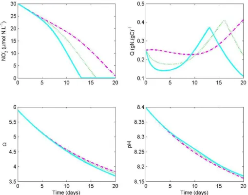
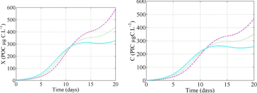
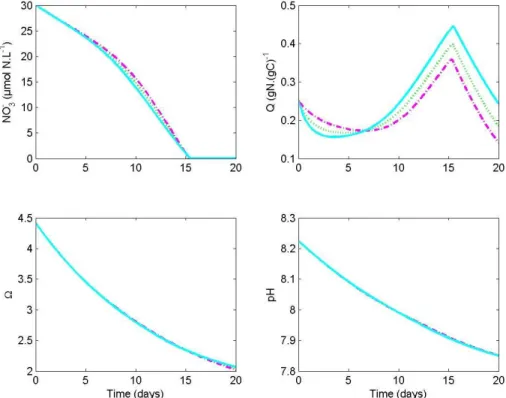
We used each of the three models to simulate a large bloom ofEmiliania huxleyi. Phy-toplankton cells are assumed to grow in a homogeneous layer, where aqueous CO2 equilibrates with the atmosphere. It takes several weeks to supply inorganic carbon

5

from both atmosphere and the deeper ocean to the cells in the whole mixed layer, and to reconstitute the stock of inorganic carbon depleted by the previous bloom (Fig. 2). The inorganic carbon stock reconstitution is slowed down by the consumption of inor-ganic carbon by theE. huxleyibloom. As a consequence, during the simulation, CO2₃− andΩshow higher values, while CO2and HCO

−

3are lower compared to their respective

10

steady state value. This fact can explain the significantly different behaviours observed between the 3 scenarii (Fig. 4). Indeed, it turns out that because of the high consump-tion of CO2 by the blooming biomass, the progressive depletion of inorganic carbon results in a stronger down regulation of growth and calcification in models controlled by CO₂or HCO−₃. On the contrary, the models regulated by CO2₃− orΩare enhanced

15

by the depletion in inorganic carbon. It results that the predicted, fixed carbon during the bloom formation is twofold in the CO2₃− andΩmodels compared to the CO2model (Fig. 4).

5.2 Simulation with doubledpCO2

Based on the accumulation rate of CO2observed in the atmosphere from the beginning

20

of the industrial era, current models roughly predict a doubling of the partial pressure of the atmospheric CO₂(pCO₂). Since the atmosphere tends to be in equilibrium with the superficial oceanic layers, changes in atmospheric CO2 show direct effects on the CO2seawater concentration, and consequently on the carbonate system speciation.

Under such conditions of elevatedpCO₂, the initial condition of depleted inorganic

25

(18)

BGD

6, 5339–5372, 2009

carbon fixation

O. Bernard et al.

Title Page

Tables Figures

◭ ◮

Back Close

Full Screen / Esc

Interactive Discussion bloom, is still transiently observed and appears more favorable to the CO2₃− and Ω

models (Fig. 5). However this tendency does not last, since inorganic carbon rapidly increases as CO₂in the water equilibrates with the elevated, atmospheric value. After one week, ambient conditions are back to high CO2concentrations and then prove to be much more favorable to the CO2 and HCO

−

3models which are then stimulated and

5

rapidly recover. Yet, important differences appear in the final PIC and POC concentra-tions, with much higher predicted values in the CO2and HCO

−

3models. 5.3 Discussion

As indicated by the coefficients of variation presented in Table 4, all models predict a two-fold difference in the final concentrations under a doubledpCO₂. Here,

simula-10

tions suggest that a change inpCO2will impact bloom formation in the coccolithophorid E. huxleyi. Yet, depending on the model, this variation is an increase (see the doubling in PIC in the CO₂ model) or a decrease (see the 45% PIC drop in the CO2₃− model). Hence, simulations also point out striking, two-fold differences in predicted concen-trations, depending on the considered regulating factor. That is, the variability in the

15

predicted values, observed between the models, equals or even exceeds that due to the rise in pCO2. This statement is reinforced when considering a tripling of pCO2 (see Table 4). This point is absolutely critical as it demonstrates the strong depen-dence of the model outcome on the initial hypotheses made as for the regulation of photosynthesis and calcification.

20

Even though schematic and academic, our simulations nevertheless integrate real-istic orders of magnitude for the underlying biological processes. The two phenom-ena, revealed by our simplified approach, are likely to appear when dealing with more realistic and accurate models as well. The tight dependence of the stock and flux predictions on the underlying regulation mechanisms and the paradoxical effect when

25

(19)

BGD

6, 5339–5372, 2009

carbon fixation

O. Bernard et al.

Title Page

Tables Figures

◭ ◮

Back Close

Full Screen / Esc

Interactive Discussion and Taylor, 1996; Merico et al.; Oguz and Merico, 2006; Gregg and Casey, 2007)

inte-grates an accurate modelling of the biological effect of apCO2 change. As stated by Riebesell (2004), it seems impossible at this point to provide any reliable forecast of large-scale and long-term biological responses to global environmental change. Our study should therefore be considered as a methodological approach on a bench model

5

to highlight a phenomenon that will take place in more detailed models (including food web interactions). As more experimental works are needed to unravel the carbon ac-quisition modes and their regulation in coccolithophorids, prediction statements should be made with caution and discussed in regard to the plausible hypotheses.

Last, another hypothesis was recently brought forward by several authors: the

cal-10

cification mechanisms also seems to be highly strain dependent (Fabry, 2008; Langer et al., 2009). As an assemblage of various strains (with different carbon acquisition regulation mechanism), a natural population would then show a range of different re-sponses to increases inpCO₂. To provide an accurate, simulated response topCO₂ change, a model should then represent each subpopulation, with various responses to

15

carbonate chemistry, so that the resulting overall response reveals to be a combination of the subpopulation behaviours. This approach may however be strongly affected by parameter uncertainties, such as the initial conditions of each subpopulation, that may jeopardize the model conclusions.

6 Conclusions

20

This study stresses how correct identification of the chemical species that drive(s) cal-cification and photosynthesis processes is critical to accurate predictions of coccol-ithophorids blooms and the consequent amount of carbon withdrawn from the atmo-sphere and trapped into the deep ocean. Model results reveal a striking difference in the predicted biomass increase when the saturation stateΩ(or equivalently CO2₃−) is

25

the regulating factor compared to the CO₂and HCO−₃models.

(20)

BGD

6, 5339–5372, 2009

carbon fixation

O. Bernard et al.

Title Page

Tables Figures

◭ ◮

Back Close

Full Screen / Esc

Interactive Discussion much lower than its value at equilibrium with the atmosphere. During these transient

phases, the scenarii in which CO2₃−orΩregulate calcification and photosynthesis may be strongly advantaged, leading thus to an unexpected effect.

The new model that we presented, in which the calcite saturation state drives calcifi-cation, turns out to be plausible alternative explanation to the CO2₃− model. This model

5

assumes that the calcite saturation state, even when higher than 1 (meaning that dis-solution rate is low), strongly influences the calcification rate. The simulation results illustrate a property that could have been shown analytically, using similar principles than in Bernard et al. (2008): theΩfollows the CO2₃− model. This model can thus ex-plain the experimental results obtained by Sciandra et al. (2003). In the hypothesis of

10

uncoupled calcification and photosynthesis, ifΩis used to control the calcification rate while the photosynthesis rate is driven by CO2, then the experimental results of Riebe-sell et al. (2000) can be reproduced. A detailed validated model may integrate more accurate knowledge, especially for carbon export, but it may also be affected by the same uncertainties that our bench model, thus resulting in highly uncertain predictions

15

of carbon fluxes in the situations of large blooms of coccolithophorids.

Results thus strongly call for further experimental approaches to more formely iden-tify the chemical species that primarily regulate photosynthesis and calcification.

Acknowledgements. The authors benefited from the support of the BOOM project (Biodiversity of Open Ocean Microcalcifiers) funded by the French National Research Agency (ANR), of the

20

European FP7 Integrated Project EPOCA (European Project on Ocean Acidification).

(21)

BGD

6, 5339–5372, 2009

carbon fixation

O. Bernard et al.

Title Page

Tables Figures

◭ ◮

Back Close

Full Screen / Esc

Interactive Discussion References

Benthien, A., Zondervan, I., Engel, A., Hefter, J., Terb ¨uggen, A., and Riebesell, U.: Carbon isotopic fractionation during a mesocosm bloom experiment dominated byEmiliania huxleyi: Effects of CO₂concentration and primary production, Geochim. Cosmochim. Ac., 71, 1528– 1541, 2007. 5351

5

Bernard, O. and Gouz ´e, J. L.: Transient Behavior of Biological Loop Models, with Application to the Droop Model, Math. Biosci., 127, 19–43, 1995. 5354

Bernard, O., Sciandra, A., and Madani, S.: Multimodel analysis of the response of the coccol-ithophore Emiliania huxleyito an elevation of pCO₂ under nitrate limitation , Ecol. Model., 211, 324–338, 2008. 5342, 5343, 5344, 5345, 5348, 5349, 5353, 5354, 5358

10

Berry, L., Taylor, A. R., Lucken, U., Ryan, K. P., and Brownlee, C.: Calcification and inorganic carbon acquisition in coccolithophores., Funct. Plant. Biol., 29, 1–11, 2002. 5341

Boyd, P. and Trull, T.: Understanding the export of biogenic particles in oceanic waters: Is there consensus?, Prog. Oceanogr., 72, 276–312, 2007. 5351

Buitenhuis, E. T., de Baar, H. J. W., and Veldhuis, M. J. V.: Photosynthesis and calcification by

15

Emiliania huxleyi(Prymnesiophyceae) as a function of inorganic carbon species., J. Phycol., 35, 949–959, 1999. 5342

Burmaster, D.: The unsteady continuous culture of phosphate-limited Monochrisis lutheri Droop: Experimental and theoretical analysis, J. Exp. Mar. Biol. Ecol., 39(2), 167–186, 1979. 5343

20

De La Rocha, C. and Passow, U.: Factors influencing the sinking of POC and the efficiency of the biological carbon pump, Deep-Sea Res. Pt. II, 54, 639–658, 2007. 5351, 5352

Droop, M. R.: Vitamin B12 and marine ecology. IV. The kinetics of uptake growth and inhibition inMonochrysis lutheri, J. Mar. Biol. Assoc. UK, 48, 689–733, 1968. 5343, 5344, 5346 Droop, M. R.: 25 Years of Algal Growth Kinetics, A Personal View, Bot. Mar., 16, 99–112, 1983.

25

5343, 5344, 5346

Dugdale, R. C.: Nutrient limitation in the sea: dynamics, identification and significance, Limnol. Oceanogr., 12, 685–695, 1967. 5344

Engel, A., Delille, B., Jacquet, S., Riebesell, U., Rochelle-Newall, E., Terbruggen, A., and Zondervan, I.: Transparent exopolymer particles and dissolved organic carbon production by

30

(22)

BGD

6, 5339–5372, 2009

carbon fixation

O. Bernard et al.

Title Page

Tables Figures

◭ ◮

Back Close

Full Screen / Esc

Interactive Discussion

Fabry, V. J.: Ocean science – Marine calcifiers in a high-CO₂ocean, Science, 320, 1020–1022, 2008. 5357

Falkowski, P. G.: Evolution of the nitrogen cycle and its influence on the biological sequestration of CO₂2 in the ocean, Nature, 327, 242–244, 1997. 5341

Frankignoulle, M., Canon, C., and Gattuso, J. P.: Marine calcification as a source of carbon

5

dioxide: positive feedback of increasing atmospheric CO₂, Limnol. Oceanogr., 39, 458–462, 1994. 5340

Gregg, W. W. and Casey, N. W.: Modeling coccolithophores in the global oceans, Deep-Sea Res. Pt. II, 54, 447–477, 2007. 5353, 5354, 5357

Harlay, J., Bodt, C. D., Engel, A., Jansen, S., d’Hoop, Q., Piontek, J., Oostende, N. V., Groom,

10

S., Sabbe, K., and Chou, L.: Abundance and size distribution of transparent exopolymer particles (TEP) in a coccolithophorid bloom in the northern Bay of Biscay, Deep-Sea Res. Pt. I, in press, 2009. 5351, 5352

Honjo, S., Manganini, S. J., Krishfield, R. A., and Francois, R.: Particulate organic carbon fluxes to the ocean interior and factors controlling the biological pump: a synthesis of global

15

sediment trap programs since 1983, Prog. Oceanogr., 76, 217–285, 2008. 5353

Houghton, J. T., Jenkins, G. J., and Ephtraims, J. J.: Climate Change 1995, The Science of Climate Change, Cambridge University Press, Cambridge, 572 pp., UK, 1996. 5341

Iglesias-Rodriguez, M. D., Halloran, P. R., Rickaby, R. E. M., Hall, I. R., Colmenero-Hidalgo, E., Gittins, J. R., Green, D. R. H., Tyrrell, T., Gibbs, S. J., von Dassow, P., Rehm, E., Armbrust,

20

E. V., and Boessenkool, K. P.: Phytoplankton Calcification in a High-CO₂₂ World, Science, 320, 336–340, 2008. 5341, 5349

Kahl, L., Vardi, A., and Schofield, O.: Effects of phytoplankton physiology on export flux, Mar. Ecol.-Prog. Ser., 354, 3–19, 2008. 5352

Keeling, R. F., Piper, S. C., and Heimann, M.: Global and hemispheric CO₂2 sinks deduced

25

from changes in atmospheric O2 concentration, Nature, 381, 308–341, 1996. 5351

Klepper, O., de Haan, B. J., and van Huet, H.: Biochemical feedbacks in the oceanic carbon cycle, Ecol. Model., 75, 459–469, 1994. 5341

Langer, G., Nehrke, G., Probert, I., Ly, J., and Ziveri, P.: Strain-specific responses of Emiliania huxleyi to changing seawater carbonate chemistry, Biogeosciences Discuss., 6, 4361–4383,

30

2009,

http://www.biogeosciences-discuss.net/6/4361/2009/. 5357

(23)

BGD

6, 5339–5372, 2009

carbon fixation

O. Bernard et al.

Title Page

Tables Figures

◭ ◮

Back Close

Full Screen / Esc

reticulata (Cryptophyta) in relation to light and nitrate-to-phosphate supply ratios, J. Phycol., 41, 567–576, 2005. 5341

Logan, B. E., Passow, U., Alldredge, A. L., Grossartt, H.-P., and Simont, M.: Rapid formation and sedimentation of large aggregates is predictable from coagulation rates (half-lives) of transparent exopolymer particles (TEP), Deep-Sea Res. Pt. II, 42, 203–214, 1995. 5352

5

Merico, A., Tyrrell, T., Lessard, E., Oguz, T., Stabeno, P., Zeeman, S., and Whitledge, T.: Modelling phytoplankton succession on the Bering Sea shelf: role of climate influences and trophic interactions in generating Emiliania huxleyi blooms 1997–2000, Deep-Sea Res. Pt. I, 51, 1803–1826, 2004. 5357

Merico, A., Tyrrell, T., and Cokacar, T.: Is there any relationship between phytoplankton

sea-10

sonal dynamics and the carbonate system?, J. Mar. Syst., 59, 120–142, 2006. 5342 Millero, F.: The Marine Inorganic Carbon Cycle, Chem. Rev., 107, 308–341, 2007. 5347 Nimer, N. and Merrett, M.: Calcification rate inEmiliania huxleyiLohmann in response to light,

nitrate and availability of inorganic carbon, New Phytol., 123, 673–677, 1993. 5346

Nimer, N. A. and Merrett, M. J.: The development of a CO₂-concentrating mechanism in

Emil-15

iania huxleyi., New Phytol., 133, 387–389, 1996. 5342

Oguz, T. and Merico, A.: Factors controlling the summerEmiliania huxleyibloom in the Black Sea: A modeling study, J. Marine Syst., 59, 173–188, 2006. 5346, 5353, 5357

Orr, J., Fabry, V., Aumont, O., Bopp, L., Doney, S., Feely, R., Gnanadesikan, A., Gruber, N., Ishida, A., Joos, F., Key, R., Lindsay, K., Maier-Reimer, E., Matear, R., Monfray, P., Mouchet,

20

A., Najjar, R., Plattner, G., Rodgers, K., Sabine, C., Sarmiento, J., Schlitzer, R., Slater, R., Totterdell, I., Weirig, M., Yamanaka, Y., and Yool, A.: Anthropogenic ocean acidification over the twenty-first century and its impact on calcifying organisms, Nature, 437, 681–686, 2005. 5341

Paasche, E.: A tracer study of the inorganic carbon uptake during coccolith formation and

25

photosynthesis in the coccolithophorid Coccolithus huxleyi., Physiol. Plantarum., 3, 1–82, 1968. 5341

Paasche, E.: A review of the coccolithophoridEmiliania huxleyi(Prymnesiophyceae), with par-ticular reference to growth, coccolith formation, and calcification-photosynthesis interaction, Phycologia, 40, 503–529, 2002. 5341

30

Passow, U. and De la Rocha, C.: Accumulation of mineral ballast on organic aggregates, Global Biogeochem. Cy., 20, GB1013, 2006. 5352

(24)

BGD

6, 5339–5372, 2009

carbon fixation

O. Bernard et al.

Title Page

Tables Figures

◭ ◮

Back Close

Full Screen / Esc

potential long-term increase of oceanic fossil fuel CO₂₂ uptake due to CO₂₂-calcification feedback, Biogeosciences, 4, 481–492, 2007,

http://www.biogeosciences.net/4/481/2007/. 5352, 5353

Riebesell, U.: Effects of CO₂₂ Enrichment on Marine Phytoplankton, J. Oceanogr., 60, 719– 729, 2004. 5342, 5357

5

Riebesell, U., Zondervan, I., Rost, B., Tortell, P., Zeebe, R. E., and Morel, F. M. M.: Reduced calcification of marine plankton in response to increased atmospheric CO₂, Nature, 407, 364–367, 2000. 5341, 5342, 5349, 5358

Riebesell, U., Wolf-Gladrow, A., and Smetacek, V.: Carbon dioxide limitation of marine phyto-plankton growth rates , Science, 361, 249–251, 1993. 5343, 5351

10

Riebesell, U., Bellerby, R. G. J., Engel, A., Fabry, V. J., Hutchins, D. A., Reusch, T. B. H., Schulz, K. G., and Morel, F. M. M.: Comment on “Phytoplankton Calcification in a High-CO₂World”, Science, 322, 1466 pp., 2008. 5341

Rost, B. and Riebesell, U.: Coccolithophores and the biological pump: responses to environ-mental changes, in: Coccolithophores. From Molecular Processes to Global Impact, edited

15

by: Thierstein, H. R. and Young, J. R., Springer, Berlin, Germany, 99–127, 2004. 5353 Rost, B., Riebesell, U., Burkhardt, S., and Sultemeyer, D.: Carbon acquisition of bloom-forming

marine phytoplankton., Limnol. Oceanogr., 48, 44–67, 2003. 5342

Rost, B., Riebesell, U., and Sultemeyer, D.: Carbon acquisition of marine phytoplankton: Effect of photoperiod length, Limnol. Oceanogr., 51, 12–20, 2006. 5342

20

Schmidt, S., Chou, L., and Hall, I.: Particle residence times in surface waters over the North-Western Iberian Margin: comparison of pre-upwelling and winter periods, J. Marine. Syst., 32, 3–11, 2002. 5353

Sciandra, A., Harlay, J., Lef ´evre, D., Lem ´ee, R., Rimmelin, P., Denis, M., and Gattuso, J.-P.: Response of coccolithophorid Emiliania huxleyito elevated partial pressure of CO₂ under

25

nitrogen limitation., Mar. Ecol. Prog. Ser., 261, 111–122, 2003. 5341, 5342, 5349, 5358 Tyrell, T. and Taylor, A.: A modelling study ofEmiliania huxleyiin the NE Atlantic , J. Marine.

Syst., 9, 83–112, 1996. 5349, 5356

Zeebe, R. E. and Wolf-Gladrow, D.: CO₂in seawater: equilibrium, kinetics, isotopes, Elsevier, 2001 pp., 2003.

30

(25)

BGD

6, 5339–5372, 2009

carbon fixation

O. Bernard et al.

Title Page

Tables Figures

◭ ◮

Back Close

Full Screen / Esc

Interactive Discussion Table 1.Definition of variables and fluxes for the four considered models .

Meaning Unit

D Dissolved inorganic carbon (DIC) mmol.L−1 N Particulate nitrogen (PON) mmol.L−1

Q Internal nitrogen quota mmol N.(mmol C)−1 X Particulate organic carbon (POC) mmol.L−1

C Coccoliths concentration (PIC) mmol.L−1

S₁ Nitrate mmol.L−1

S₂ Calcium mmol.L−1

Ω Calcite saturation state –

(26)

BGD

6, 5339–5372, 2009

carbon fixation

O. Bernard et al.

Title Page Abstract Introduction Conclusions References Tables Figures ◭ ◮ ◭ ◮ Back Close

Full Screen / Esc

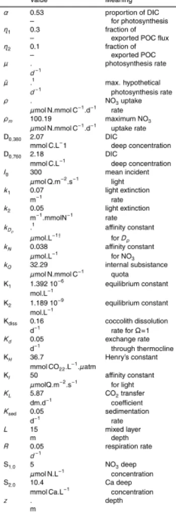
Interactive Discussion Table 2. Definitions and values of the model parameters. 1: depends on the model type, see

Table 3.†: unitless forΩ.

Value Meaning

α 0.53 proportion of DIC – for photosynthesis

η1 0.3 fraction of

– exported POC flux

η2 0.1 fraction of

– exported POC

µ . photosynthesis rate

d−1

¯

µ .1 _{max. hypothetical}

d−1 _{photosynthesis rate}

ρ . NO3uptake

µmol N.mmol C−1_.d−1 _rate

ρm 100.19 maximum NO3

µmol N.mmol C−1_.d−1 _{uptake rate}

D0,380 2.07 DIC

mmol C.L−

1 deep concentration D0,760 2.18 DIC

mmol C.L−1 _{deep concentration}

I0 300 mean incident

µmol Q.m−2_.s−1 _light

k1 0.07 light extinction

m−1 _rate

k2 0.05 light extinction

m−1_.mmolN−1 _rate

kDp .

1 _a

ffinity constant

µmol.L−1†

forDp kN 0.038 affinity constant

µmol.L−1 _{for NO} 3

kQ 32.29 internal subsistance µmol N.mmol C−1 _quota

K1 1.392 10

−6 _{equilibrium constant}

mol.L−1

K2 1.189 10

−9 _{equilibrium constant}

mol.L−1

Kdiss 0.16 coccolith dissolution

d−1 _{rate for}

Ω=1

Kd 0.05 exchange rate

d−1 _{through thermocline}

KH 36.7 Henry’s constant

mmol CO22.L

−1_._µ_atm

KI 50 affinity constant µmolQ.m−2_.s−1 _{for light}

KL 5.87 CO2transfer

dm.d−1 _coe

fficient

Ksed 0.05 sedimentation

d−1 _rate

L 15 mixed layer m depth

R 0.05 respiration rate

d−1

S1,0 5 NO3deep

µmol N.L−1 _{concentration}

S2,0 10.4 Ca deep

mmol Ca.L−1 _{concentration}

(27)

BGD

6, 5339–5372, 2009

carbon fixation

O. Bernard et al.

Title Page

Tables Figures

◭ ◮

Back Close

Full Screen / Esc

Interactive Discussion Table 3. Kinetics parameters depending on the chosen model (†: unitless fork_Ω)

.

Parameters CO2₃− HCO−₃ CO₂ Ω Units

k_D

p 0.076 1.65 0.015 3.23

†

µmol C.L−1 ¯

µ 1.34 0.96 1.7 1.64 d−1

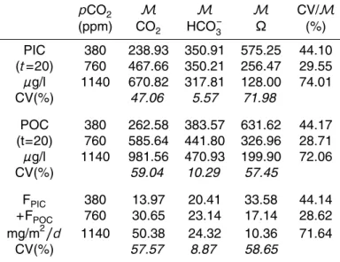
Table 4. Final values of PIC and POC att=20 days, and average dayly exported carbon during the bloom, in mg C.m−2.d−1with respect to the considered model andpCO₂. CV: coefficient of variation (expressed in %).

pCO₂ M M M CV/M

(ppm) CO₂ HCO−₃ Ω (%) PIC 380 238.93 350.91 575.25 44.10 (t=20) 760 467.66 350.21 256.47 29.55

µg/l 1140 670.82 317.81 128.00 74.01

CV(%) 47.06 5.57 71.98

POC 380 262.58 383.57 631.62 44.17 (t=20) 760 585.64 441.80 326.96 28.71

µg/l 1140 981.56 470.93 199.90 72.06

CV(%) 59.04 10.29 57.45

F_PIC 380 13.97 20.41 33.58 44.14

+F_POC 760 30.65 23.14 17.14 28.62 mg/m2/d 1140 50.38 24.32 10.36 71.64

(28)