ACPD
11, 10935–10972, 2011Potential evaporation trends
C. Matsoukas et al.
Title Page
Abstract Introduction
Conclusions References
Tables Figures
◭ ◮
◭ ◮
Back Close
Full Screen / Esc
Printer-friendly Version Interactive Discussion
Discussion
P
a
per
|
Dis
cussion
P
a
per
|
Discussion
P
a
per
|
Discussio
n
P
a
per
|
Atmos. Chem. Phys. Discuss., 11, 10935–10972, 2011 www.atmos-chem-phys-discuss.net/11/10935/2011/ doi:10.5194/acpd-11-10935-2011
© Author(s) 2011. CC Attribution 3.0 License.
Atmospheric Chemistry and Physics Discussions
This discussion paper is/has been under review for the journal Atmospheric Chemistry and Physics (ACP). Please refer to the corresponding final paper in ACP if available.
Potential evaporation trends over land
between 1983–2008: driven by radiative or
turbulent fluxes?
C. Matsoukas1, N. Benas2, N. Hatzianastassiou3, K. G. Pavlakis4, M. Kanakidou5, and I. Vardavas2
1
Department of Environment, University of the Aegean, Mytilene, Greece
2
Department of Physics, University of Crete, Heraklion, Greece
3
Laboratory of Meteorology, Department of Physics, University of Ioannina, Ioannina, Greece
4
Department of General Applied Science, Technological Educational Institute of Crete, Heraklion, Greece
5
Environmental Chemical Processes Laboratory, Department of Chemistry, University of Crete, Heraklion, Greece
Received: 11 February 2011 – Accepted: 28 March 2011 – Published: 8 April 2011
Correspondence to: C. Matsoukas ([email protected])
ACPD
11, 10935–10972, 2011Potential evaporation trends
C. Matsoukas et al.
Title Page
Abstract Introduction
Conclusions References
Tables Figures
◭ ◮
◭ ◮
Back Close
Full Screen / Esc
Printer-friendly Version Interactive Discussion
Discussion
P
a
per
|
Dis
cussion
P
a
per
|
Discussion
P
a
per
|
Discussio
n
P
a
per
|
Abstract
We model the Penman potential evaporation (PE) over all land areas of the globe for the 25-year period 1983–2008, relying on radiation transfer models (RTMs) for the shortwave and longwave fluxes. Penman’s PE is determined by two factors: avail-able energy for evaporation and ground to atmosphere vapour transfer. Input to the 5
PE model and RTMs comprises satellite cloud and aerosol data, as well as data from reanalyses. PE is closely linked to pan evaporation, whose trends have sparked contro-versy in the community, since the factors responsible for the observed pan evaporation trends are not determined with consensus. Our particular interest is the temporal evo-lution of PE, and the provided insight to the observed trends of pan evaporation. We 10
examine the interannual trends of PE and various related physical quantities, such as net solar flux, net longwave flux, water vapour saturation deficit and wind speed. Our findings are the following: Global warming has led to a larger water vapour saturation deficit. Global dimming/brightening cycles in the last 25 years slightly increased the available energy for evaporation. PE trends seem to follow closely the trends of energy 15
availability and not the trends of the atmospheric capability for vapour transfer, almost everywhere on the globe, with trends in the Northern hemisphere significantly larger than in the Southern. These results support the hypothesis that secular changes in the radiation fluxes, and not vapour transfer considerations, are responsible for potential evaporation trends.
20
1 Introduction
There have been many reports on significant changes in pan evaporation for widespread locations across the globe, e.g. European Russia, Siberia, and the USA (Peterson et al., 1995; Golubev et al., 2001), India (Chattopadhyay and Hulme, 1997), the USA (Lawrimore and Peterson, 2000), Israel (Cohen et al., 2002), China (Liu et al., 25
ACPD
11, 10935–10972, 2011Potential evaporation trends
C. Matsoukas et al.
Title Page
Abstract Introduction
Conclusions References
Tables Figures
◭ ◮
◭ ◮
Back Close
Full Screen / Esc
Printer-friendly Version Interactive Discussion
Discussion
P
a
per
|
Dis
cussion
P
a
per
|
Discussion
P
a
per
|
Discussio
n
P
a
per
|
2007), and many others (references in Roderick et al. (2007) and Fu et al. (2009)). However, a study for Australia (Jovanovic et al., 2008) cast some doubt on the veracity of the Australian trends. It reported that unaccounted discontinuities (e.g. the installa-tion of bird meshes) produced a spurious declining trend, which disappears if the time series are homogenised. There is a need for similar studies in other regions, but until 5
they are carried out, the emerging general picture is one of worldwide decreasing pan evaporation, with some exceptions, e.g. east USA, a single pan in Israel, central Aus-tralia, etc. However, Global Circulation Model (GCM) runs on the one hand (Wetherald and Manabe, 2002), and reanalyses (Trenberth et al., 2005) and empirical hydrological evidence (Huntington, 2006) on the other, dictate that in a warming world the hydrolog-10
ical cycle should be enhanced and evaporation should increase.
This disagreement between the trends of actual evaporation and pan evaporation was termed the “evaporation paradox” and was initially addressed when Brutsaert and Parlange (1998) brought forward the complementary hypothesis, already proposed by Bouchet (1963) and applied by Morton (1975). It consists of the following reason-15
ing: in humid environments, with ample supply of moisture to the surface, the actual evaporation takes values close to the potential evaporation. Also, the pan evaporation corresponds directly to the potential evaporation, after multiplication with the pan co-efficient. However, in arid environments actual evaporation cannot reach the values of potential evaporation, and therefore a larger portion of the available energy takes 20
the form of sensible heat flux, thus warming the atmosphere. The warmer atmosphere now is characterized by the apparent potential evaporation, which is larger than the po-tential evaporation at the same water-limited location. The pan evaporation is related to the apparent potential evaporation. In these lines, if the available energy for evapo-ration is constant, an increase in actual evapoevapo-ration decreases the sensible heat flux, 25
ACPD
11, 10935–10972, 2011Potential evaporation trends
C. Matsoukas et al.
Title Page
Abstract Introduction
Conclusions References
Tables Figures
◭ ◮
◭ ◮
Back Close
Full Screen / Esc
Printer-friendly Version Interactive Discussion
Discussion
P
a
per
|
Dis
cussion
P
a
per
|
Discussion
P
a
per
|
Discussio
n
P
a
per
|
(2001) after deriving actual evaporation rates over the former Soviet Union and the USA, also find the complementary hypothesis reasonable. Zhang et al. (2007) calcu-lated potential and actual evaporation from 16 watersheds in the Tibetan plateau and analysed them for the validity of the complementary hypothesis. They found indica-tions for the existence of a complementary relaindica-tionship, although weaker than the one 5
originally proposed by Bouchet (1963).
However, during the same period an alternate theory appeared. Stanhill and Cohen (2001) showed that the solar irradiance had been declining the past decades (global dimming), with potential influences on the evaporation. Cohen et al. (2002) in an Is-rael case study, argued that the known sensitivity of pan evaporation to net radiation 10
at the surface is enough to explain its decrease in a globally dimming world. They proposed that aerosol and cloud-induced global dimming is the main reason for the general downward trend of the pan evaporation, because the vapour pressure deficit (VPD) was displaying increasing trends, contrary to the expectations of the comple-mentary hypothesis. Roderick and Farquhar (2002) supported the global dimming so-15
lution to the paradox, showing that the recent solar flux decrease is enough to account for the pan evaporation trend in a former Soviet Union area. Linacre (2004) in a study with simplified global average changes of temperature, dew point temperature, so-lar radiation, agrees that global dimming is the major factor in the decreases of pan evaporation. Wild et al. (2004) showed Global Energy Balance Archive (GEBA) data, 20
indicating that the net shortwave and longwave radiation available for evaporation has been declining. In order to reconcile the decreasing radiative energy with the increas-ing temperature observations, they conclude that the hydrological cycle (and thus the evaporative cooling) has to weaken. Therefore, they disagree with the complementary hypothesis, which requires enhanced evaporation. The global dimming has reversed 25
ACPD
11, 10935–10972, 2011Potential evaporation trends
C. Matsoukas et al.
Title Page
Abstract Introduction
Conclusions References
Tables Figures
◭ ◮
◭ ◮
Back Close
Full Screen / Esc
Printer-friendly Version Interactive Discussion
Discussion
P
a
per
|
Dis
cussion
P
a
per
|
Discussion
P
a
per
|
Discussio
n
P
a
per
|
To further complicate the picture, case studies in Australia (Roderick et al., 2007) and the Tibetan plateau (Zhang et al., 2007) showed that neither radiation trends, nor humidity issues were the major factor in pan evaporation trends. Instead the authors attribute the change to wind speed decreases. Johnson and Sharma (2010) calculated the pan evaporation trend in Australia from station, reanalysis and GCM data. Although 5
the station data identified the wind change as the factor with the strongest contribution to the trend, the reanalysis data attributed the trend mostly to water vapour deficit change. However, it still remains to be seen if the effect of the wind has a regional or even global character.
Brutsaert (2006) has proposed that the reported decreases in pan evaporation can 10
be attributed partly to solar dimming and partly to actual evaporation increases via the complementary relationship. In other words the two hypotheses do not have to be mu-tually exclusive. Teuling et al. (2009) have found that evaporation depends on different drivers, in regions of Europe and North America. In drier water-limited regions, such as South Europe and the US Southwest, evaporation follows the interannual fluctuations 15
of precipitation, while in wetter energy-limited regions, such as central and North Eu-rope and the American Northeast, evaporation follows in suite with global dimming and brightening. Therefore, evaporation can be increasing or decreasing with decreasing pan evaporation, depending on the location. For example, global dimming in energy-limited areas, will cause both pan evaporation and actual evaporation to decrease. On 20
the other hand, a positive precipitation trend in water-limited regions, will increase ac-tual evaporation, but decrease pan evaporation. Teuling et al. (2009) agree that the two hypotheses do not have to be mutually exclusive.
A recent review by Fu et al. (2009) on the subject lists the significant problems asso-ciated with each of the two explanations of the paradox, i.e. solar dimming and comple-25
ACPD
11, 10935–10972, 2011Potential evaporation trends
C. Matsoukas et al.
Title Page
Abstract Introduction
Conclusions References
Tables Figures
◭ ◮
◭ ◮
Back Close
Full Screen / Esc
Printer-friendly Version Interactive Discussion
Discussion
P
a
per
|
Dis
cussion
P
a
per
|
Discussion
P
a
per
|
Discussio
n
P
a
per
|
1990 years, when a reversal from global dimming to global brightening is noted. Fourth, the relationship between pan evaporation and reference potential evaporation needs to be further clarified. Fifth, the separate study of land and ocean evaporation trends. Sixth, they highlight that the crux of the problem is the trend of the actual evaporation and we need to find ways to advance our knowledge there.
5
In this work, we focus on the potential (open-water) evaporation rate over all land areas of the planet. In order to estimate it, we assume the existence of a small shallow water body in each land location. The hypothetical water body has to be small, so that the regional climate can be considered undisturbed, and shallow, so that heat storage considerations can be ignored. The open water evaporation from this small, shallow 10
water body can be assumed to be the (apparent) potential evaporation at the same location. Our objectives here are the accurate calculation of potential evaporation over land areas, derivation of its regional trends, and quantification of the contribution of solar decadal fluctuations and water vapour transfer changes to the potential evapora-tion trends. The link of potential evaporaevapora-tion to the pan evaporaevapora-tion will provide some 15
insight to the pan evaporation decadal changes.
In more detail, we will analyse the monthly potential evaporation for years 1983– 2008, in a spatial 2.5◦
×2.5◦resolution, over all land areas of the globe. We use our
ra-diation transfer models for solar and thermal longwave rara-diation, already employed in a variety of climatic studies (Hatzianastassiou and Vardavas, 1999, 2001a,b; Hatzianas-20
tassiou et al., 1999, 2004a,b, 2005, 2007a,b; Pavlakis et al., 2004, 2007, 2008; Var-davas and Taylor, 2007; Matsoukas et al., 2010) for the calculation of the necessary radiation fluxes. We also employ reanalysis humidity, wind and temperature data, in order to calculate the evaporation component due to mass transfer processes. We are thus in a position to include both parameters in our analysis: net radiation fluxes 25
ACPD
11, 10935–10972, 2011Potential evaporation trends
C. Matsoukas et al.
Title Page
Abstract Introduction
Conclusions References
Tables Figures
◭ ◮
◭ ◮
Back Close
Full Screen / Esc
Printer-friendly Version Interactive Discussion
Discussion
P
a
per
|
Dis
cussion
P
a
per
|
Discussion
P
a
per
|
Discussio
n
P
a
per
|
analysis. Priority three, because our period of study extends well beyond 1990. In Matsoukas et al. (2005, 2007), we touched upon priority five, but due to lack of inter-annual, spatially distributed heat storage data in the oceans, the trend of general ocean evaporation is beyond our reach.
2 Methodology and data
5
Our objective is to estimate the monthly potential evaporation globally over all land areas in 2.5◦
×2.5◦resolution. In each 2.5◦×2.5◦cell the aerodynamic evaporation rate Eais estimated from
Ea=UCw(es−e) (1)
whereU is the scalar wind,esthe saturation water vapour pressure at the 2 m temper-10
ature, andethe observed water vapour pressure at 2 m. The differencees−eis the
vapour pressure deficit (VPD).Cw is a turbulent exchange coefficient, estimated by a variety of methods, e.g. Brutsaert (1982, chap. 4), Winter et al. (1995). The derivation ofCw is relatively simple for neutral atmospheric stability conditions, but once
atmo-spheric instability is included in the analysis, it becomes considerably more complex. 15
Neglecting air stability issues in the estimation of potential evaporation can lead to seri-ous errors when the time resolution is finer than 24 h. However, for resolutions coarser than daily, the errors tend to cancel out and the assumption of neutral stability works well (Mahrt and Ek, 1993; Brutsaert, 1982, p. 217). Since our approach uses monthly values, we assume that using the neutral form of Cw is sufficient. We have verified
20
the validity of the above assumption for the evaporation of the Mediterranean Sea in Matsoukas et al. (2005). For its calculation we use the following method from Brutsaert (1982)
Cw=
0.622avk2 RdTalnz2
z0υln
z1 z0m
ACPD
11, 10935–10972, 2011Potential evaporation trends
C. Matsoukas et al.
Title Page
Abstract Introduction
Conclusions References
Tables Figures
◭ ◮
◭ ◮
Back Close
Full Screen / Esc
Printer-friendly Version Interactive Discussion
Discussion
P
a
per
|
Dis
cussion
P
a
per
|
Discussion
P
a
per
|
Discussio
n
P
a
per
|
with k=0.41 the von K ´arm ´an constant, av=1.13 the ratio of von K ´arm ´an constants for water and wind,Rdthe specific gas constant for dry air, Tathe air temperature, z1
and z2 the measurement heights for wind speed and humidity, and z0υ and z0m the
roughness lengths for water vapour and momentum.
The aerodynamically derived evaporation Ea is one model of the evaporative pro-5
cess, taking into account only the drying power of air. It has the advantage of requir-ing as input few and easily available physical quantities, i.e. air temperature, humidity, wind speed, air pressure. All these data were taken in a monthly, 0.5◦
×0.5◦
resolu-tion from the European Centre for Medium Range Forecast (ECMWF) Re-Analyses, namely ERA-40 (Uppala et al., 2005) up to August 2002 and the latest ERA Interim 10
for the period January 1989–June 2008. The main objectives of ERA Interim were “to improve on certain key aspects of ERA-40, such as the representation of the hydrolog-ical cycle, the quality of the stratospheric circulation, and the handling of biases and changes in the observing system” (Berrisford et al., 2009), including wind measure-ments, which is of specific interest in this study. ERA data were regridded to 2.5◦
×2.5◦
15
resolution, in order to match the radiation transfer model resolution.
Another way to model evaporation is through the energy balance method, which estimates the available energy Rn for the turbulent fluxes (evaporation and sensible heat) using the principle of energy conservation:
Rn=Qs−Ql−∆H−G (3)
20
whereQs is the net solar energy flux, Ql the net terrestrial flux corresponding to ra-diative cooling, G is the energy flux advected away from the surface, and ∆H is the stored heat assumed. Since our model is applied to a shallow water body,∆H can be neglected (Brutsaert, 1982, p. 153). Also, for monthly resolutionsGis relatively small and can be considered negligible (Shuttleworth, 1993).
25
The energy balance evaporation rateEr, which corresponds toRn is
Er=
Rn
ACPD
11, 10935–10972, 2011Potential evaporation trends
C. Matsoukas et al.
Title Page
Abstract Introduction
Conclusions References
Tables Figures
◭ ◮
◭ ◮
Back Close
Full Screen / Esc
Printer-friendly Version Interactive Discussion
Discussion
P
a
per
|
Dis
cussion
P
a
per
|
Discussion
P
a
per
|
Discussio
n
P
a
per
|
whereρis the density of water andLits latent heat of evaporation, estimated by
L=2.501×10⁶−2350Ta(J kg−1) (5)
with the air temperatureTain◦C.
Chow et al. (1988, pp. 86–87) state that “the evaporation may be computed by the aerodynamic method when energy supply is not limiting and by the energy balance 5
method when vapour transport is not limiting. But, normally, both of these factors are limiting so a combination of the two methods is needed”. Doing just that, the method developed by Penman (1948) gives the evaporation rateEpas a weighted average of
Er andEa, using the formula
Ep= ∆
∆ +γEr+ γ
∆ +γEa (6)
10
where∆is the slope of the saturation water vapour pressure curve at the air tempera-tureTa, andγ is the psychrometric constant
γ= cpp
0.622L (7)
withcpthe moist air heat capacity andpthe atmospheric pressure.
Penman’s method has consistently ranked among the best methods for the calcula-15
tion of potential evaporation over water bodies. Chow et al. (1988, pp. 86–89) classified it as the best evaporation method when all relevant data are available and the neces-sary assumptions are justified. Winter et al. (1995), Rosenberry et al. (2004, 2007) found it one of three best out of at least eleven methods in the cases of Lake Williams in Minnesota, a prairie wetland in North Dakota, and a small mountain lake in the north-20
ACPD
11, 10935–10972, 2011Potential evaporation trends
C. Matsoukas et al.
Title Page
Abstract Introduction
Conclusions References
Tables Figures
◭ ◮
◭ ◮
Back Close
Full Screen / Esc
Printer-friendly Version Interactive Discussion
Discussion
P
a
per
|
Dis
cussion
P
a
per
|
Discussion
P
a
per
|
Discussio
n
P
a
per
|
ones that are not measured at every meteorological station are the radiation fluxesQs
and Ql. Therefore, using radiation transfer models to calculate them everywhere on the globe, is our only recourse.
2.1 Radiative transfer model description
The deterministic 1-D spectral radiative transfer model used here was developed from 5
a radiative-convective model (Vardavas and Carver, 1984; Vardavas and Taylor, 2007). The sky is divided into clear and cloudy fractions. The cloudy fraction includes three non-overlapping layers of low, mid and high-level clouds. The model input data include cloud amounts (for low, mid, high-level clouds), cloud scattering and absorption optical depths, cloud-top pressure and temperature (for each cloud type), cloud geometrical 10
thickness and vertical temperature and specific humidity profiles. For the total amount of ozone, carbon dioxide, methane, and nitrous oxide in the atmosphere, we used the same values as in Hatzianastassiou and Vardavas (2001a).
All of the cloud climatological data for our radiation transfer model were taken from the International Satellite Cloud Climatology Project (ISCCP-D2) data set (Rossow 15
and Schiffer, 1999), which provides monthly means for 72 climatological variables in 2.5◦
×2.5◦, monthly resolution, for 15 cloud types and for the 25-year period July 1983–
June 2008. ISCCP converts 30 km×30 km cloud data every 3 h to an equal-area map
grid with 280 km resolution. The Stage D2 data product is produced by further averag-ing over each month, first at each of the eight 3 h time slots and then over all time slots. 20
The cloud-top temperature is derived from the infrared radiances, while the cloud-top pressure from the vertical temperature profile of the atmosphere.
The water vapour and temperature vertical atmospheric profiles, used in the ra-diative transfer model, come from the National Centers for Environmental Prediction (NCEP)/National Center for Atmospheric Research (NCAR) global reanalysis project 25
(Kistler et al., 2001), corrected for topography as in Hatzianastassiou and Vardavas (2001a). These data are also on a 2.5◦ resolution, monthly averaged and cover the
ACPD
11, 10935–10972, 2011Potential evaporation trends
C. Matsoukas et al.
Title Page
Abstract Introduction
Conclusions References
Tables Figures
◭ ◮
◭ ◮
Back Close
Full Screen / Esc
Printer-friendly Version Interactive Discussion
Discussion
P
a
per
|
Dis
cussion
P
a
per
|
Discussion
P
a
per
|
Discussio
n
P
a
per
|
Our radiation transfer model is accordingly customised and applied in two different radiation domains, the shortwave (SW, solar) and the longwave (LW, terrestrial). Below, we present briefly the two separate models.
2.1.1 Shortwave radiation transfer model
The incoming solar irradiance conforms to the spectral profile of Thekaekara and Drum-5
mond (1971) and corresponds to a solar constantS0 of 1367 Wm−2 (Willson, 1997;
Hartmann, 1994, p. 23). The model makes adjustments for the elliptical Earth orbit and apportions 69.48% of the incoming spectral irradiance to the ultra violet–visible–near infrared (UV-Vis-NIR) part (0.20–1 µm) and 30.52% to the near infrared–infrared (NIR-IR) part (1–10 µm). Then, the radiative transfer equations are solved for 118 separate 10
wavelengths for the UV-Vis-NIR part and for 10 bands for the NIR-IR part, using the Delta-Eddington method of Joseph et al. (1976). For a more detailed model description the reader is referred to Hatzianastassiou et al. (2004b,a, 2007a,b).
The model takes into account Rayleigh scattering due to atmospheric gas molecules, as well as absorption from O3, CO2, H2O, and CH4. The O3 column amount is 15
taken from the Television Infrared Observational Satellite (TIROS) Operational Verti-cal Sounder (TOVS). Complete aerosol data are provided by the Global Aerosol Data Set (GADS) (K ¨opke et al., 1997).
The model output can include downwelling and upwelling fluxes at the top of atmo-sphere, at the surface and at any atmospheric height. The focus of this study is the 20
solar energy absorbed at the surface, or net (downwelling minus reflected) flux at the surface. As mentioned above, in this study we use the fluxes absorbed by a hypotheti-cal shallow water body on the ground. Therefore, in the estimation of the net shortwave flux we use the water surface albedo, modelled using Fresnel reflection as a function of the solar zenith angle and corrected for a non-smooth surface.
ACPD
11, 10935–10972, 2011Potential evaporation trends
C. Matsoukas et al.
Title Page
Abstract Introduction
Conclusions References
Tables Figures
◭ ◮
◭ ◮
Back Close
Full Screen / Esc
Printer-friendly Version Interactive Discussion
Discussion
P
a
per
|
Dis
cussion
P
a
per
|
Discussion
P
a
per
|
Discussio
n
P
a
per
|
2.1.2 Longwave radiation transfer model
The detailed radiative-convective model developed for climate change studies of Var-davas and Carver (1984) is modified for the radiation transfer of terrestrial infrared radiation, in order to compute the downwelling longwave radiation (DLR) and upwelling fluxes at the surface of the Earth. The model has monthly, 2.5◦
×2.5◦ resolution
(dic-5
tated from the resolution of ISCCP-D2) and a vertical resolution of 5 mb, from the sur-face up to 50 mb, to ensure that the atmospheric layers are optically thin with respect to the Planck mean longwave opacity. The atmospheric molecules considered are H2O, CO2, CH4, O3, and N2O. The sky is divided into clear and cloudy fractions. The cloudy fraction includes three non-overlapping layers of low, mid and high-level clouds. The 10
model input data include cloud amounts (for low, mid, high-level clouds), cloud scatter-ing and absorption optical depths, cloud-top pressure and temperature (for each cloud type), cloud geometrical thickness and vertical temperature and specific humidity pro-files.
A full presentation and discussion of an earlier version of the model can be found in 15
Pavlakis et al. (2004). There, a series of sensitivity tests were performed to investigate how much uncertainty is introduced in the model DLR by uncertainties in the input pa-rameters, such as air temperature, skin temperature, low, middle or high cloud amount as well as the cloud physical thickness, cloud overlap schemes, and the use of daily-mean instead of monthly-daily-mean input data. The model DLR was also validated against 20
ACPD
11, 10935–10972, 2011Potential evaporation trends
C. Matsoukas et al.
Title Page
Abstract Introduction
Conclusions References
Tables Figures
◭ ◮
◭ ◮
Back Close
Full Screen / Esc
Printer-friendly Version Interactive Discussion
Discussion
P
a
per
|
Dis
cussion
P
a
per
|
Discussion
P
a
per
|
Discussio
n
P
a
per
|
3 Results
3.1 Long-term average
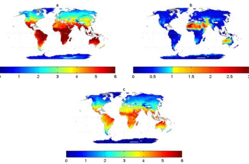
We start by using Eq. (1) to compute the bulk aerodynamic evaporationEafor the globe,
with input data (air temperature, humidity, wind speed, air pressure) originating from ERA-40 and ERA Interim. This quantity corresponds only to mass transfer procedures 5
and assumes unlimited energy availability. A long-term average (July 1983–June 2002) of the annualEa, calculated from ERA-40 data is presented in Fig. 1 (top left), showing maxima over generally dry areas, such as deserts and minima over wetter and colder areas. A direct comparison with the long-term annual average of the VPD in Fig. 1 (top right), shows the qualitative resemblance withEaand highlights the dominance of 10
the VPD in the geographical distribution of aerodynamic evaporation. The long-term annual average of wind speed is shown in Fig. 1 (bottom). The regional patterns of
U and Ea do not correlate very well, indicating that the wind speed U plays only a secondary role in the bulk aerodynamic evaporation regional distribution. This is also true for the the exchange coefficientCw.
15
We proceed by calculating the available energyRnfor turbulent processes, i.e. evap-oration and sensible heat flux. As mentioned before, this energy is derived from our radiative models, run over fictitious small and shallow water bodies at each location. If we assume that all this energy flux is used up in evaporation, we obtain the evapo-ration rateEr, whose global distribution is shown in Fig. 2 (top left). A comparison of 20
Ea in Fig. 1 (top left) with Er in Fig. 2 (top left) shows that there are two very distinct processes that govern potential evaporation. In some dry locationsEa is larger than
Er, meaning that the available energy does not suffice to maintain the potential evapo-ration rate dictated by mass transfer and potential evapoevapo-ration is energy limited there. This is highlighted in Fig. 2 (top right), where we present the ratio Ea/Er. In areas 25
ACPD
11, 10935–10972, 2011Potential evaporation trends
C. Matsoukas et al.
Title Page
Abstract Introduction
Conclusions References
Tables Figures
◭ ◮
◭ ◮
Back Close
Full Screen / Esc
Printer-friendly Version Interactive Discussion
Discussion
P
a
per
|
Dis
cussion
P
a
per
|
Discussion
P
a
per
|
Discussio
n
P
a
per
|
potential evaporation there is vapour transfer limited.
Penman’s method (Eq. 6) takes into account the two processes and derives a more accurate estimateEpof the potential evaporation. The long-term averageEpis shown in Fig. 2 (bottom), with its expected latitudinal gradient, its maximum values close to the Equator, its poleward decrease and its minimal values in Antarctica and Greenland. 5
Ep follows closelyEr, because∆ is usually larger thanγ in Eq. (6) and therefore the
Er contribution toEpdominates the Ea contribution in all but the coldest regions. The global average of the potential evaporation of small shallow water bodies over land areas for July 1983 to June 2002 is 2.6 mm day−1.
3.2 Global trends
10
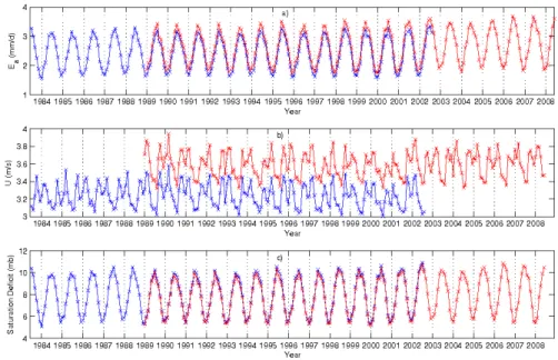
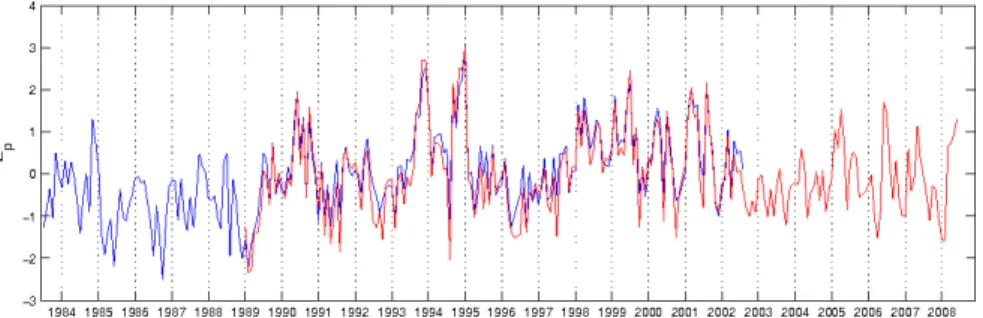
We now focus on the interannual behaviour of global potential evaporation, as well as the quantities that affect it, namely wind speed, VPD, net solar flux and net terres-trial flux. In this study “global” means the area-weighted average of land-only values. We first present in Fig. 3a the evolution of global mean bulk aerodynamic evaporation
Ea, calculated by Eq. (1), using data from ERA-40 (blue line) and ERA Interim (red 15
line). There is a consistent difference between the two time series during the tempo-ral overlap between January 1989 and August 2002, when data were available from both ERA-40 and Interim. The reason for the larger Interim values is the consistently increased wind speeds compared to ERA-40, as can be seen in Fig. 3b). Except from the wind speed, the global means of the other relevant quantities (2 m air temperature, 20
dew point temperature, VPD) do not show significant differences between ERA-40 and Interim. For example, in Fig. 3c we show the time series of the VPD global mean, where the two lines are very close.
Fitting linear trends to raw time series, such as the ones in Fig. 3, is not a good prac-tice, because the large seasonal fluctuations hide possible trends and keep them from 25
ACPD
11, 10935–10972, 2011Potential evaporation trends
C. Matsoukas et al.
Title Page
Abstract Introduction
Conclusions References
Tables Figures
◭ ◮
◭ ◮
Back Close
Full Screen / Esc
Printer-friendly Version Interactive Discussion
Discussion
P
a
per
|
Dis
cussion
P
a
per
|
Discussion
P
a
per
|
Discussio
n
P
a
per
|
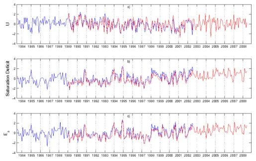
a more robust trend analysis, we take the deseasonalised time series, normalised by the standard deviation of the interannual variability for each specific month. For ex-ample, the normalised anomaly of June 2001 is the difference between the June 2001 value and the mean of all June values, divided by the standard deviation of all June values. In this fashion we have derived normalised plots for wind speedU, VPD, and 5
bulk aerodynamic evaporationEa(Fig. 4), net solar flux Qs, net terrestrial fluxQl, and energy balance evaporationEr (Fig. 5), and Penman potential evaporation (Fig. 6).
As expected, the seasonality of the quantities is not apparent in these plots and we can proceed to check if interannual trends are present globally over land. Also, the differences between normalised anomalies of ERA-40 and Interim for quantitiesU, 10
VPD,Ea, andEp(Figs. 4 and 6), seem small and non-systematic. Therefore, for each one of the aforementioned quantities, we generated a “blended” time series with only ERA-40 normalised anomalies for July 1983–December 1988, the average of ERA-40 and Interim normalised anomalies for the overlapping period of January 1989–August 2002, and ERA Interim only for September 2002–June 2008. These “blended” time 15
series will be used for the rest of the paper in order to calculate linear trends for the relevant variablesU,es−e,Ea, andEp.
There seems to be a wind speed decrease in the 90’s, which has stopped (if not reversed) around 2000. The VPD seems to be increasing since the 90’s, as doesEa
(but less steeply). Trends inQs,Ql,Er, andEpare not very obvious and dependent on 20
the choice of the period of interest and its start and end points.Ql in particular displays an increasing trend in the last two decades.
Fitting linear trends to the generated normalised anomaly time series produces the trend values shown in Table 1. The numbers in italics mean that the 95% confidence interval of the slope does not contain zero. The normalised anomalies have also been 25
averaged over North and South Hemispheres and their trends are presented sepa-rately.
ACPD
11, 10935–10972, 2011Potential evaporation trends
C. Matsoukas et al.
Title Page
Abstract Introduction
Conclusions References
Tables Figures
◭ ◮
◭ ◮
Back Close
Full Screen / Esc
Printer-friendly Version Interactive Discussion
Discussion
P
a
per
|
Dis
cussion
P
a
per
|
Discussion
P
a
per
|
Discussio
n
P
a
per
|
apparent in Fig. 4b), driving the bulk aerodynamic evaporationEatrend to positive sta-tistically significant values. AlthoughQsshows a positive trend in the late eighties and throughout the nineties (solar brightening), after 2000 this trend has levelled off(Wild et al., 2009). In the full period (July 1983–June 2008) there remains a weak but statis-tically significant increase in the net solar heating of the surface. The radiative cooling 5
of the surfaceQl is increasing more steeply thanQs. The same sign of trends in solar heating and thermal radiation cooling cause a statistically non significant change in the net energy flux at the surface, therefore Er has a weak, non significant trend. How-ever, our result for the apparent potential evaporation Ep over land areas, estimated by Penman’s method, is a statistically significant increase over the last decades. The 10
ratioEa/Er is also increasing with statistical significance, indicating a potential evapo-ration that is less limited by vapour transfer, but more limited by energy fluxes. In other words, the VPD has increased, resulting in a more vapour-hungry atmosphere, but the net energy at the surface has not increased as much as to satisfy this demand. All above trends are stronger in the North Hemisphere than either globally or in the South 15
Hemisphere. In SH the only statistically significant trends are found for VPD and Ea. On the other hand, in NH all examined quantities seem to be significantly changing, with the wind speed decreasing and everything else increasing.
There is a general reluctance to derive trends from reanalysis data. The main reason is that the observational data assimilated by the reanalysis scheme may at some times 20
be less dense than other times, or that the assimilation scheme may be revised. These changes could produce spurious, statistically significant trends. However, we decided to use reanalysis data for the calculation of Ep trends for two reasons. First, ERA Interim starts in 1989, when satellite data were mature, global and abundant, leading us to expect small changes in data coverage and density. Second, reanalysis data 25
trends affect mainly Ea and not Er. As we note above, Ep depends weakly on Ea,
ACPD
11, 10935–10972, 2011Potential evaporation trends
C. Matsoukas et al.
Title Page
Abstract Introduction
Conclusions References
Tables Figures
◭ ◮
◭ ◮
Back Close
Full Screen / Esc
Printer-friendly Version Interactive Discussion
Discussion
P
a
per
|
Dis
cussion
P
a
per
|
Discussion
P
a
per
|
Discussio
n
P
a
per
|
3.3 Geographically resolved trends
We compile monthly timeseries at every 2.5◦
×2.5◦cell of the globe for the period July
1983–June 2008. Each individual timeseries is transformed to a normalised anomaly timeseries and fitted with a least-squares line. For quantities originating from both ERA-40 and Interim, a blended normalised anomaly time series has been calculated 5
and all plots and results reported here are derived from it. Each slope is tested for difference from zero with statistical significance at 95% confidence level. Below, we present the regional distribution of these trends for potential evaporation and all other relevant physical quantities. Only statistically significant slopes are presented. The normalised anomalies are unitless. An interpretation of the values of quantities in the 10
following trend plots (Figs. 7 and 8) is the change per decade of the difference of the quantity from its interannual monthly mean over its interannual monthly standard deviation.
Examining the regional wind trends, it is apparent that in the last 25 years wind speeds are generally decreasing everywhere except Antarctica, scattered parts of 15
North America and East Asia, extended parts of South America and North Africa, cen-tral Europe, the Kalahari, Indochina and Indonesia. These trends are in agreement (at least qualitatively) with Roderick et al. (2007), Zhang et al. (2007), and McVicar et al. (2008). McVicar et al. (2008) point out that Australian stations and ERA-40 reanalysis data agree well in wind climatologies, but the reanalysis trends are weaker than the 20
station ones. Our ERA analysis is also in agreement with Pryor et al. (2009), who how-ever find differences in reanalysis and station trends for the contiguous US and show scepticism in using reanalysis data for trend detection. We understand the difficulties in substituting local wind measurements with reanalysed data, but we should also note that there is no consensus on the magnitude of wind trends in Australia, even between 25
station-only analyses (Jovanovic et al., 2008).
The bulk aerodynamic evaporationEa and the VPD (i.e. es−e) are globally on the
ACPD
11, 10935–10972, 2011Potential evaporation trends
C. Matsoukas et al.
Title Page
Abstract Introduction
Conclusions References
Tables Figures
◭ ◮
◭ ◮
Back Close
Full Screen / Esc
Printer-friendly Version Interactive Discussion
Discussion
P
a
per
|
Dis
cussion
P
a
per
|
Discussion
P
a
per
|
Discussio
n
P
a
per
|
Africa and various scattered small regions throughout the globe. Only statistically sig-nificant trends are shown in Figs. 7 and 8. The VPD trend is caused by the fact that in ERA both air temperatureT and dew point temperatureTdare rising, butT is doing so faster thanTd(results not shown). The positive trend ofTdshows that the water cycle
is intensifying, but not enough to decrease the VPD in a warming world. This increase 5
in the “drying capacity” of air runs contrary to the complementary hypothesis.
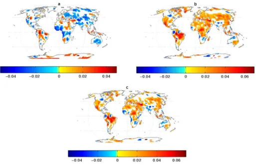
The globe seems to be divided in half with respect to the prevalence of global dim-ming or global brightening in the period July 1983–June 2008. Decadal changes in net solar heating Qs led to less radiation (dimming) in parts of Canada, Greenland, North Eurasia, East Asia, most of Australia, and Antarctica (not shown, but very similar 10
to Fig. 8a). All other areas witnessed brightening. The surface seems to be radiat-ing increasradiat-ingly net longwave fluxQl during the examined period, contributing to less available energy for evaporation. Exceptions are West South America, West Africa, West Australia, Central Eurasia, Indonesia and scattered spots in various locations (not shown). The combined trends ofQs and Ql produced the trend of Er, shown in 15
Fig. 8a. The general image is similar to the trends in Qs, indicating that the major player in radiative flux changes is the solar energy and not the terrestrial longwave. Also, Penman potential evaporationEpregional trends in Fig. 8b agree quite well with
Er in Fig. 8a. In some regions, opposite signs of trends in Er and Ea have removed statistical significance inEpchanges, e.g. parts of Greenland and North-east Asia, but 20
the differences between the two figures are small.
4 Discussion: is potential evaporation driven by energy or mass transfer issues?
Let us revisit the two competing hypotheses on the decreasing pan evaporation trends. On the one hand the complementary hypothesis proposes that changes in the water 25
ACPD
11, 10935–10972, 2011Potential evaporation trends
C. Matsoukas et al.
Title Page
Abstract Introduction
Conclusions References
Tables Figures
◭ ◮
◭ ◮
Back Close
Full Screen / Esc
Printer-friendly Version Interactive Discussion
Discussion
P
a
per
|
Dis
cussion
P
a
per
|
Discussion
P
a
per
|
Discussio
n
P
a
per
|
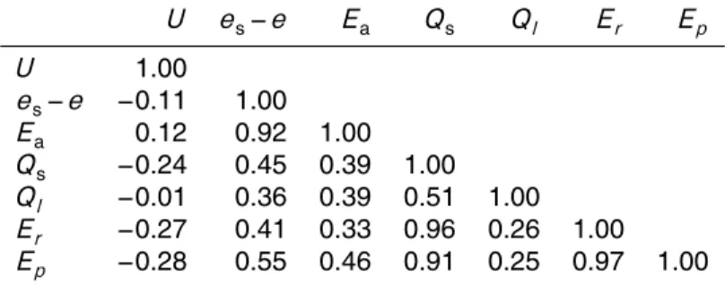
for the pan evaporation trends. In order to provide some insight into this problem, it is important to elucidate the relationships between the deseasonalised, normalised trends ofU, es−e, Ea, Qs, Ql, Er and Ep. To this end, we compile Table 2 with the cross-correlation coefficientsR2between all possible pairs of the above quantities.
We will examine the values greater than 0.5, namely the ones corresponding to the 5
pairs Ea–VPD, Qs-Ql, Er-Qs, Ep-VPD, Ep-Qs and Ep-Er. The large correlation of Ea
and VPD has been inferred previously in this study, by the similarities in both their regional distributions and their global normalised anomalies.QsandQl are correlated because of their common relationship to cloud cover. For example, when clouds are present, they obstruct both net solar heating and terrestrial cooling, leading to smaller 10
values ofQl andQs. The long-term global average values ofQsandQl are respectively 150 W m−2and 48 W m−2, soQ
sdominatesQl. If we also take into account Eqs. 3 and 4, the close relationship ofErwithQsis not surprising. Finally, we have already pointed out the stronger relationship ofEpwithEr, rather than withEa, due to the usually larger
coefficient ofEr in Eq. (6). Notably, with a 0.97 correlation coefficient, we can see that 15
Penman’s potential evaporation Ep trend is almost exclusively dictated by the trend of the available energy Er. The Ep-Ea correlation is not negligible, but rather weak
compared to the pairEp-Er.
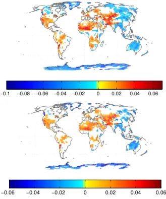
This result is examined further, by presenting the geographically distributed cross-correlation between deseasonalised and normalised trends of Ep on the one hand 20
and Er or Ea on the other, in Fig. 9. The very strong cross-correlation found for the global normalised, deseasonalised trends ofEpand Er (top of Fig. 9) in the previous paragraph seems very robust. In most areas this correlation coefficient is above 0.9, with some exceptions in the Sahara, Greenland (where it is still larger than 0.8) and parts of Antarctica. Ep trends are dominated by Ea trends only in parts of the latter 25
ACPD
11, 10935–10972, 2011Potential evaporation trends
C. Matsoukas et al.
Title Page
Abstract Introduction
Conclusions References
Tables Figures
◭ ◮
◭ ◮
Back Close
Full Screen / Esc
Printer-friendly Version Interactive Discussion
Discussion
P
a
per
|
Dis
cussion
P
a
per
|
Discussion
P
a
per
|
Discussio
n
P
a
per
|
This finding comes to the support of the hypothesis that global dimming/brightening controls the trends in potential and pan evaporation. The bulk aerodynamic evaporation
Ea is also positively correlated with the potential evaporation Ep, but this effect is of principal importance only in parts of Antarctica. The energy balance evaporationEr is not totally independent ofEa, so all three quantities are linked. However, the degree 5
ofEr and Ep trend correlation is very prominent and provides a clear answer. In this study, the available energy (mainly solar) is the driver for potential (and consecutively pan) evaporation trends in our dataset and not water vapour transfer.
5 Conclusions
Pan and potential evaporation are directly proportional and therefore a study on po-10
tential evaporation can shed some light on the factors that affect the much discussed observed trends of pan evaporation. We use Penman’s method to calculate the po-tential evaporation for all land areas of the globe in a monthly 2.5◦
×2.5◦ resolution.
Penman’s method is widely recognised as one of the most accurate calculations of potential evaporation. It takes into account two relevant processes: the drying power 15
of the air (the water vapour transfer potential) and the energy available to the evapora-tion process. Penman’s method then compromises the two sometimes conflicting pro-cesses and produces an estimate for potential evaporation. Since it requires modelling of both radiative and turbulent fluxes, it is data intensive and needs quantities (e.g. net radiation fluxes), which are not readily measured in all world regions. We employ radi-20
ation transfer models as a way to circumvent the problem of radiative flux availability. In order to run the radiative transfer models we need data for clouds (ISCCP-D2), aerosol (GADS), and atmospheric temperature and humidity profiles (NCEP/NCAR reanaly-sis). ECMWF reanalysis data (ERA-40 and ERA Interim) are used for the turbulent flux model.
25
ACPD
11, 10935–10972, 2011Potential evaporation trends
C. Matsoukas et al.
Title Page
Abstract Introduction
Conclusions References
Tables Figures
◭ ◮
◭ ◮
Back Close
Full Screen / Esc
Printer-friendly Version Interactive Discussion
Discussion
P
a
per
|
Dis
cussion
P
a
per
|
Discussion
P
a
per
|
Discussio
n
P
a
per
|
of pan evaporation. We examine the interannual trends of potential evaporation and various related physical quantities, such as net solar flux, net longwave flux, vapour pressure deficit (VPD) and wind speed. Trends of reanalysis quantities, which are related to turbulent fluxes, such as the VPD, wind, and bulk aerodynamic evaporation
Ea, should be reported carefully because of possible changes in data coverage and 5
assimilation techniques during the reanalysis period and the consequent generation of spurious trends. In our case, we think spurious effects are minimal because data coverage changes are small after 1989, with satellites routinely providing uninterrupted global coverage. Moreover, Penman potential evaporation depends weakly on turbulent fluxes but more strongly on radiative fluxes, which are less sensitive to reanalyses. 10
Atmospheric temperature, dew point temperature, and vapour pressure deficit (VPD) appear to be globally increasing. The increase of dew point temperature is an indication of an enhanced water cycle, in line with the complementary hypothesis. However, the agreement stops here, because the temperature is increasing even faster than the dew point temperature, resulting in decreasing relative humidity and increasing VPD and 15
Ea.
Global dimming/brightening cycles in these 25 years increased the available solar energy, driving the total energy available for evaporation to larger values. Radiative longwave cooling also increased, having the opposite to solar (but smaller) effect on total available energy. The energy balance evaporationEr is proportional to this avail-20
able energy for evaporation and therefore it has a positive trend. The ratio Ea/Er is also increasing with statistical significance, indicating a potential evaporation that is less limited by vapour transfer, but more limited by energy fluxes. All above trends are stronger in the North Hemisphere than either globally or in the South Hemisphere. In SH the only statistically significant trends are found for VPD andEa. On the other hand, 25
in NH all examined quantities seem to be significantly changing, with the wind speed decreasing and everything else increasing.
ACPD
11, 10935–10972, 2011Potential evaporation trends
C. Matsoukas et al.
Title Page
Abstract Introduction
Conclusions References
Tables Figures
◭ ◮
◭ ◮
Back Close
Full Screen / Esc
Printer-friendly Version Interactive Discussion
Discussion
P
a
per
|
Dis
cussion
P
a
per
|
Discussion
P
a
per
|
Discussio
n
P
a
per
|
geographically robust, with the exception of Antarctica, where there is a mixed picture. The results above tend to support the hypothesis that secular changes in the radiation fluxes are responsible for potential evaporation trends, and not vapour transfer issues, such as the ones proposed by the complementary hypothesis.
Acknowledgements. The ISCCP D2 data were obtained from the International Satellite Cloud
5
Climatology Project web site http://isccp.giss.nasa.gov maintained by the ISCCP research group at the NASA Goddard Institute for Space Studies, New York, NY. The GADS aerosol data were obtained from the Meteorological Institute of the University of Munich. NCEP/NCAR Reanalysis Derived data provided by the NOAA/OAR/ESRL PSD, Boulder, Colorado, USA, from their Web site at http://www.cdc.noaa.gov/. ERA-40 and Interim reanalysis data were
10
provided by the European Centre for Medium-Range Weather Forecast (ECMWF) and down-loaded from http://www.ecmwf.int/. Part of this work has been performed in the frame of the European Union Integrated Project CIRCE (contract no. 036961).
References
Berrisford, P., Dee, D., Fielding, K., Fuentes, M., K ˚allberg, P., Kobayashi, S., and Uppala, S.:
15
The ERA-Interim archive, vol. 1 ofERA report series, ECMWF, Shinfield Park, Reading, UK, 2009. 10942
Bouchet, R. J.: ´Evapotranspiration r ´eelle et potentielle. Signification climatique, Tech. Rep. 62, Int. Assoc. Sci. Hydrol., 1963. 10937, 10938
Brutsaert, W.: Evaporation into the atmosphere, Reidel, Dordrecht, The Netherlands, 299 pp.,
20
edn. 1991, ISBN 90-277-1247-6., 1982. 10941, 10942
Brutsaert, W. and Parlange M. B.: Hydrologic cycle explains the evaporation paradox, Nature, 396, p. 30, 1998. 10937
Brutsaert, W.: Indications of increasing land surface evaporation during the second half of the 20th century, Geophys. Res. Lett., 33, L20403, doi:10.1029/2006GL027532, 2006. 10939
25
Chattopadhyay, N. and Hulme, M.: Evaporation and potential evapotranspiration in India under conditions of recent and future climate change, Agric. For. Meteorol., 87, 55–73, 1997. 10936 Chow, V. T., Maidment, D. R., and Mays, L. W.: Applied Hydrology, McGraw-Hill, New York,
ACPD
11, 10935–10972, 2011Potential evaporation trends
C. Matsoukas et al.
Title Page
Abstract Introduction
Conclusions References
Tables Figures
◭ ◮
◭ ◮
Back Close
Full Screen / Esc
Printer-friendly Version Interactive Discussion
Discussion
P
a
per
|
Dis
cussion
P
a
per
|
Discussion
P
a
per
|
Discussio
n
P
a
per
|
Cohen, S., Ianetz, A., and Stanhill, G.: Evaporative climate changes at Bet Dagan, Israel, 1964–1998, Agric. For. Meteorol., 111, 83–91, 2002. 10936, 10938
Fu, G., Charles, S. P., and Yu, J.: A critical overview of pan evaporation trends over the last 50 years, Clim. Change, 97, 193–214, doi:10.1007/s10584-009-9579-1, 2009. 10937, 10939, 10940
5
Golubev, V. S., Lawrimore, J. H., Groisman, P. Y., Speranskaya, N. A., Zhuravin, S. A., Menne, M. J., Peterson, T. C., and Malone, R. W.: Evaporation changes over the contiguous United States and the former USSR: A reassessment, Geophys. Res. Lett., 28, 2665–2668, 2001. 10936, 10937
Hartmann, D. L.: Global physical climatology, Academic Press, London, UK, 411 pp., ISBN
10
0-12-328530-5, 1994. 10945
Hatzianastassiou, N. and Vardavas, I.: Shortwave radiation budget of the Northern Hemisphere using International Satellite Cloud Climatology Project and NCEP/NCAR climatological data, J. Geophys. Res., 104(D20), 24401–24421, 1999. 10940
Hatzianastassiou, N. and Vardavas, I.: Shortwave radiation Budget of the Southern
Hemi-15
sphere using ISCCP C2 and NCEP-NCAR climatological data, J. Climate, 14, 4319–4329, 2001a. 10940, 10944
Hatzianastassiou, N. and Vardavas, I.: Longwave radiation budget of the Southern Hemisphere using ISCCP C2 climatological data, J. Geophys. Res., 106(D16), 17785–17798, 2001b. 10940
20
Hatzianastassiou, N., Croke, B., Kortsalioudakis, N., Vardavas, I., and Koutoulaki, K.: A model for the longwave radiation budget of the NH: Comparison with Earth Radiation Budget Ex-periment data, J. Geophys. Res., 104(D8), 9489–9500, 1999. 10940
Hatzianastassiou, N., Katsoulis, B., and Vardavas, I.: Global distribution of aerosol direct radia-tive forcing in the ultraviolet and visible arising under clear skies, Tellus, 56B, 51–71, 2004a.
25
10940, 10945
Hatzianastassiou, N., Matsoukas, C., Hatzidimitriou, D., Pavlakis, C., Drakakis, M., and Var-davas, I.: Ten-year radiation budget of the Earth: 1984–1993, Int. J. Climatol., 24, 1785– 1802, doi:10.1002/joc.1110, 2004b. 10940, 10945
Hatzianastassiou, N., Matsoukas, C., Fotiadi, A., Pavlakis, K. G., Drakakis, E., Hatzidimitriou,
30
D., and Vardavas, I.: Global distribution of Earth’s surface shortwave radiation budget, Atmos. Chem. Phys., 5, 2847–2867, doi:10.5194/acp-5-2847-2005, 2005. 10940
ACPD
11, 10935–10972, 2011Potential evaporation trends
C. Matsoukas et al.
Title Page
Abstract Introduction
Conclusions References
Tables Figures
◭ ◮
◭ ◮
Back Close
Full Screen / Esc
Printer-friendly Version Interactive Discussion
Discussion
P
a
per
|
Dis
cussion
P
a
per
|
Discussion
P
a
per
|
Discussio
n
P
a
per
|
A., Pavlakis, K. G., and Vardavas, I.: The direct effect of aerosols on solar radiation based on satellite observations, reanalysis datasets, and spectral aerosol optical properties from Global Aerosol Data Set (GADS), Atmos. Chem. Phys., 7, 2585–2599, doi:10.5194/acp-7-2585-2007, 2007a. 10940, 10945
Hatzianastassiou, N., Matsoukas, C., Fotiadi, A., P. W. Stackhouse Jr., Koepke, P., Pavlakis, K.
5
G., and Vardavas, I.: Modelling the direct effect of aerosols in the solar near-infrared on a planetary scale, Atmos. Chem. Phys., 7, 3211–3229, doi:10.5194/acp-7-3211-2007, 2007b. 10940, 10945
Huntington, T. G.: Evidence for intensification of the global water cycle: Review and synthesis, J. Hydrol., 319, 83–95, 2006. 10937
10
Johnson, F. and Sharma, A.: A comparison of Australian open water body evaporation trends for current and future climates estimated from Class A evaporation pans and General Circu-lation Models, J. Hydrometeorol., 11, 105–121, doi:10.1175/2009JHM1158.1, 2010. 10939 Joseph, J. H., Wiscombe, W. J., and Weinmann, J. A.: The Delta- Eddington approximation of
radiative flux transfer, J. Atmos. Sci., 33, 2452–2459, 1976. 10945
15
Jovanovic, B., Jones, D. A., and Collins, D.: A high-quality monthly pan evaporation dataset for Australia, Climatic Change, 87, 517–535, doi:10.1007/s10584-007-9324-6, 2008. 10937, 10951
Kistler, R., Kalnay, E., Collins, W., Saha, S., White, G., Woolen, J., Chelliah, M., Ebisuzaki, W., Kanamitsu, M., Kousky, V., van den Dool, H., Jenne, R., and Fiorino, M.: The
NCEP-20
NCAR 50-year reanalysis: Monthly means CD-ROM and documentation, Bull. Amer. Meteo-rol. Soc., 82, 247–268, 2001. 10944
K ¨opke, P., Hess, M., Schult, I., and Shettle, E. P.: Global Aerosol Data Set, Tech. Rep. 234, Max Planck Institute f ¨ur Meteorologie, 1997. 10945
Lawrimore, J. H. and Peterson, T. C.: Pan evaporation trends in dry and humid regions of the
25
United States, J. Hydrol., 1, 543–546, 2000. 10936, 10937
Linacre, E. T.: Evaporation trends, Theor. Appl. Climatol., 79, 11–21, 2004. 10938
Liu, B., Xu, M., Henderson, M., and Gong, W.: A spatial analysis of pan evaporation trends in China, 1955–2000, J. Geophys. Res., 109, D15102, doi:10.1029/2004JD004511, 2004. 10936
30
Mahrt, L. and Ek, M.: The influence of atmospheric stability on potential evaporation, J. Climate Appl. Meteor., 23, 222–234, 1993. 10941
ACPD
11, 10935–10972, 2011Potential evaporation trends
C. Matsoukas et al.
Title Page
Abstract Introduction
Conclusions References
Tables Figures
◭ ◮
◭ ◮
Back Close
Full Screen / Esc
Printer-friendly Version Interactive Discussion
Discussion
P
a
per
|
Dis
cussion
P
a
per
|
Discussion
P
a
per
|
Discussio
n
P
a
per
|
E., Stackhouse, P. W., and Vardavas, I.: Seasonal energy budget of the Mediterranean Sea, J. Geophys. Res., 110, C12008, doi:10.1029/2004JC002566, 2005. 10941, 10946
Matsoukas, C., Banks, A. C., Pavlakis, K. G., Hatzianastassiou Jr., N. P. W. S., and Vardavas, I.: Seasonal heat budgets of the Red and Black seas, J. Geophys. Res., 112, C10017, doi:10.1029/2006JC003849, 2007. 10941
5
Matsoukas, C., Hatzianastassiou, N., Fotiadi, A., Pavlakis, K. G., and Vardavas, I.: The effect of Arctic sea-ice extent on the absorbed (net) solar flux at the surface, based on ISCCP-D2 cloud data for 1983-2007, Atmos. Chem. Phys., 10, 777–787, doi:10.5194/acp-10-777-2010, 2010. 10940
McVicar, T. R., Niel, T. G. V., Li, L. T., Roderick, M. L., Rayner, D. P., Ricciardulli, L., and
10
Donohue, R. J.: Wind speed climatology and trends for Australia, 1975–2006: Capturing the stilling phenomenon and comparison with near-surface reanalysis output, Geophys. Res. Lett., 35, L20403, doi:10.1029/2008GL035627, 2008. 10951
Morton, F. I.: Estimating evaporation and transpiration from climatological observations, J. Appl. Meteorol., 14, 488–497, 1975. 10937
15
Pavlakis, K. G., Hatzidimitriou, D., Matsoukas, C., Drakakis, E., Hatzianastassiou, N., and Vardavas, I.: Ten-year global distribution of downwelling longwave radiation, Atmos. Chem. Phys., 4, 127–142, doi:10.5194/acp-4-127-2004, 2004. 10940, 10946
Pavlakis, K. G., Hatzidimitriou, D., Drakakis, E., Matsoukas, C., Fotiadi, A., Hatzianastassiou, N., and Vardavas, I.: ENSO surface longwave radiation forcing over the tropical Pacific,
20
Atmos. Chem. Phys., 7, 2013–2026, doi:10.5194/acp-7-2013-2007, 2007. 10940
Pavlakis, K. G., Hatzianastassiou, N., Matsoukas, C., Fotiadi, A., and Vardavas, I.: ENSO surface shortwave radiation forcing over the tropical Pacific, Atmos. Chem. Phys., 8, 5565– 5577, doi:10.5194/acp-8-5565-2008, 2008. 10940
Penman, H. L.: Natural evaporation from open water, bare soil and grass, Proc. Roy. Soc.
25
London, A193, 120–146, 1948. 10943
Peterson, T. C., Golubev, V. S., and Groisman, P. Y.: Evaporation losing its strength, Nature, 377, 687–688, 1995. 10936
Pryor, S. C., Barthelmie, R. J., Young, D. T., Takle, E. S., Arritt, R. W., Flory Jr., D. W. J. G., Nunes, A., and Roads, J.: Wind speed trends over the contiguous United States, J. Geophys.
30
Res., 114, D14105, doi:10.1029/2008JD011416, 2009. 10951
ACPD
11, 10935–10972, 2011Potential evaporation trends
C. Matsoukas et al.
Title Page
Abstract Introduction
Conclusions References
Tables Figures
◭ ◮
◭ ◮
Back Close
Full Screen / Esc
Printer-friendly Version Interactive Discussion
Discussion
P
a
per
|
Dis
cussion
P
a
per
|
Discussion
P
a
per
|
Discussio
n
P
a
per
|
Roderick, M. L. and Farquhar, G. D.: Changes in Australian pan evaporation from 1970 to 2002, Int. J. Climatol., 24, 1077–1090, doi:10.1002/joc.1061, 2004. 10936
Roderick, M. L., Rotstayn, L. D., Farquhar, G. D., and Hobbins, M. T.: On the attribution of changing pan evaporation, Geophys. Res. Lett., 34, L17403, doi:10.1029/2007GL031166, 2007. 10937, 10939, 10951
5
Rosenberry, D. O., Stannard, D. I., Winter, T. C., and Martinez, M. L.: Comparison of 13 equa-tions for determining evapotranspiration from a prairie wetland, Cottonwood Lake Area, North Dakota, USA, Wetlands, 24, 483–497, 2004. 10943
Rosenberry, D. O., Winter, T. C., Buso, D. C., and Likens, G. E.: Comparison of 15 evaporation methods applied to a small mountain lake in the northeastern USA, J. Hydrol., 340, 149–166,
10
doi:10.1016/j.jhydrol.2007.03.018, 2007. 10943
Rossow, W. B. and Schiffer, R. A.: Advances in understanding clouds from ISCCP, Bull. Amer. Meteorol. Soc., 80, 2261–2286, 1999. 10944
Shuttleworth, W. J.: Evaporation, in: Handbook of Hydrology, edited by: Maidment, D. R., McGraw-Hill, 4.1–4.53, New York, USA, 1993. 10942
15
Stanhill, G. and Cohen, S.: Global dimming: a review of the evidence for a widespread and significant reduction in global radiation with discussion of its probable causes and possible agricultural consequences, Agric. For. Meteorol., 107, 255–278, 2001. 10938
Tanny, J., Cohen, S., Assouline, S., Lange, F., Grava, A., Berger, D., Teltch, B., and Parlange, M. B.: Evaporation from a small water reservoir: Direct measurements and estimates, J.
20
Hydrol., 351, 218–229, doi:10.1016/j.jhydrol.2007.12.012, 2008. 10943
Teuling, A. J., Hirschi, M., Ohmura, A., Wild, M., Reichstein, M., Ciais, P., Buchmann, N., Ammann, C., Montagnani, L., Richardson, A. D., Wohlfahrt, G., and Seneviratne, S. I.: A regional perspective on trends in continental evaporation, Geophys. Res. Lett., 36, L02404, doi:10.1029/2008GL036584, 2009. 10939
25
Thekaekara, M. P. and Drummond, A. J.: Standard values for the solar constant and its spectral components, Nat. Phys. Sci., 229, 6–9, 1971. 10945
Trenberth, K. E., Fasullo, J., and Smith, L.: Trends and variability in column-integrated atmo-spheric water vapor, Clim. Dynam., 24, 741–758, doi:10.1007/s00382-005-0017-4, 2005. 10937
30