*e-mail: [email protected]
Received: 20 December 2015 / Accepted: 20 June 2016
Estimating the mechanical competence parameter of the
trabecular bone: a neural network approach
Érica Regina Filletti*, Waldir Leite Roque
Abstract Introduction: The mechanical competence parameter (MCP) of the trabecular bone is a parameter that merges the volume fraction, connectivity, tortuosity and Young modulus of elasticity, to provide a single measure of the trabecular bone structural quality. Methods: As the MCP is estimated for 3D images and the Young modulus simulations are quite consuming, in this paper, an alternative approach to estimate the MCP based on artiicial neural network (ANN) is discussed considering as the training set a group of 23 in vitro vertebrae and 12 distal radius samples obtained by microcomputed tomography (μCT), and 83 in vivo distal radius magnetic resonance image samples (MRI). Results: It is shown that the ANN was able to predict with very high accuracy the MCP for 29 new samples, being 6 vertebrae and 3 distal radius bones by μCT and 20 distal radius bone by MRI. Conclusion: There is a strong correlation (R2 = 0.97) between both techniques and,
despite the small number of testing samples, the Bland-Altman analysis shows that ANN is within the limits of agreement to estimate the MCP.
Keywords: Osteoporosis, Trabecular bone, Mechanical competence, Artiicial neural network, Machine learning.
Introduction
Osteoporosis is a prevalent disease among the elderly population and due to the increase in life expectancy it is becoming a public health problem
with very high cost to both public and private health
systems (Dimai et al., 2012). Osteoporosis causes
a remarkable bone mass loss and trabecular bone degradation, which normally leads to an increase in bone fragility and an augmented fracture risk. One of
the main functions of the bone is to support or bear loads applied on it. For this reason, it should be strong
enough to avoid breakage and keep its stiffness. Therefore, it is important to known about bone strength and stiffness, particularly when investigating
the effect of different external stimuli.
It is now known that the trabecular microarchitecture degradation impacts the fragility fracture risk. The trabecular bone structure is organized as a network of rod-like and plate-like struts forming a tortuous grid, which inluences the mechanical behavior of the
structure. Recently, in (Roque et al., 2013a; Roque et al., 2013b) it was shown that the trabecular bone volume
fraction (BV/TV), the network connectivity (EPC), the trabecular tortuosity (τ) and the elasticity (E) are
relevant parameters to establish the trabecular bone mechanical competence. Using these four parameters, by means of the principal component analysis (PCA),
a mechanical competence parameter (MCP) was
deined and applied to grade trabecular bone fragility
for three different cohorts.
Principal component analysis (PCA) is a technique
that reduces a complex data set to a lower dimension to reveal the sometimes hidden, simpliied structure
that often underlie it. The variable reduction is
applicable only when there is a strong correlation between the data sets (Jolliffe, 2002). The linear
correlation analysis of the parameters BV/TV, EPC, τ and E, has shown to be very high. When the PCA
is applied to these four trabecular bone parameters, it merges morphological, geometrical and mechanical information about the trabecular bone structure into
a unique parameter. The MCP was deined as the
principal component in the PCA.
Artiicial neural network (ANN) is a technique
that has attracted much attention as an approach to
estimate quantities when there are complex relationships between input and output variables, particularly when no links are known among them a priori. Amongst
several advantages of neural network models, it can
be emphasized that they are easy to use and to update, possess large degree of freedom and give accurate prediction at high speed (Nafey, 2009; Niemi et al., 1995). The main one is the ability to generalize, i.e.,
to learn from examples. In this regard, after an ANN
has been satisfactorily trained and tested, it is able to
Filletti ÉR, Roque WL
predict the output of new input data in the domain covered by the training examples. In addition, ANNs can also include available theoretical knowledge about
the process. As a consequence, some researchers have devoted their time to study the application of neural
networks models to the trabecular bone characterization
and strength analysis.
Christopher and Ramakrishnan (2007) evaluated the mechanical strength of the trabecular structure of the human femur using digital processing of images
obtained by radiographs and artiicial neural networks
to classify normal or abnormal bone structure.
The results have shown that the method is able to
provide useful information about the strength of the femur trabecular structure. Gregory et al. (1999) have
used the Fourier transform and neural networks to
identify changes in the structure of the trabecular bone. Hambli (2011) developed an approach based
on inite element methods and neural networks to estimate the density and length of cracks in trabecular bone. The results have shown a good qualitative agreement compared with experimental results
published previously.
In this regard, in a previous study (Filletti and Roque, 2015), the authors investigated the application
of an ANN to predict the MCP for 20 magnetic
resonance image (MRI) samples based on a training
set of 83 in vivo distal radius MRI samples. The ANN
was able to predict the MCP of the test samples with a relative average error of 6.5%. As the ANN was applied to a set of in vivo distal radius MRI
samples, in this paper an investigation on how the ANN responds to a set of samples from different
bone sites, vertebrae and distal radius, using MRI and
μCT as two different imagery techniques is carried out. The results obtained by the ANN have shown to be very satisfactory, with a relative average error of 11%, when considering as the training set both
bone samples merged in a unique set. Therefore,
while the paper Filletti and Roque (2015) had only
distal radius bone samples with MRI, in this paper it is shown that the ANN can estimate the MCP
for a more general case, including samples that originate from different bone sites and different imaging techniques.
Thus, this paper shows that the ANN technique
can be extended to estimate the MCP for the trabecular
bone from different sites and imaging devices without appealing to calculate it through PCA. Once the ANN is trained, it will provide a simple, accurate and faster
method to estimate the MCP, thus avoiding PCA,
which is a much more laborious technique.
Methods
To investigate the potentiality of the ANN, the current work considers three different cohorts. Two in vitro
μCT sets of trabecular bone 3D image samples: one set
from distal radius containing 15 images and another
containing 29 L3 vertebral samples. The inal isotropic resolution was 34μm and the analyzed direction was
craniocaudal to the vertebrae and distal-proximal to
the radius. These two set of trabecular bone samples were obtained from human cadavers following all the
technical procedure requirements. Additional details can be found in Roque and Alberich-Bayarri (2015), Arcaro (2013) and references therein.
The third cohort was composed of 103 MRI radius
samples from in vivo human subjects, captured from the distal metaphysis and from a cohort including healthy subjects and a mix of bone mineral density
stages, which includes osteopenic and osteoporotic subjects. The MRI acquisitions were performed in a 3 Tesla system, scanned in 3D using a T1-weighted gradient echo sequence (TE/TR/a=5 ms/16 ms/25 Å) and with a nominal isotropic resolution of 180 μm.
Full details about all these samples can be found in (Roque et al., 2013b).
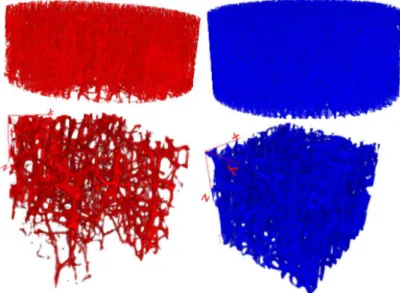
Figure 1 shows 3D images of two pair of trabecular
bone samples, vertebral bodies at the top and distal radius at the bottom. On the left side, for both, it can be noticed that the structures are more disrupted than those on the right side, due to the advanced
osteoporosis. Figure 2 shows 3D images of two distal radius trabecular bone samples, with the image on
the right side more disrupted.
Mechanical competence parameter
Principal component analysis (PCA) technique for
variable reduction is applicable only when there is a strong correlation between these variables (Jolliffe, 2002). In (Roque et al., 2013a) the mechanical
competence parameter (MCP) was deined to grade the
trabecular bone fragility by means of four trabecular bone fundamental quantities: volume fraction (BV/TV),
network connectivity via the volumetric Euler-Poincaré
characteristic (EPCV), tortuosity (τ) and the Young
modulus of elasticity (E).
In this paper, the MCP was applied to grade
the TB fragility of the three cohorts (Roque and Alberich-Bayarri, 2015), with the distal radius μCT samples given by
MCP
DR = 0.52 × BV/TV – 0.49 × EPCV +
0.51 × E – 0.48 × τ, (1)
MCP for the vertebrae μCT samples is given by
MCPV = 0.55 × BV/TV – 0.48 × EPCV +
0.50 × E – 0.47 × τ, (2)
and MCP for the MRI distal radius samples is given by
MCPMRDR = 0.53 × BV/TV – 0.50 × EPCV +
0.51 × E – 0.45 × τ. (3)
Once the four parameters are provided in Equations
1, 2 and 3, the MCP for each set of samples can be determined. To set the range of the MCP in the interval
[0, 1], a normalization procedure is deined as
k MIN N
MAX MIN
MCP MCP
MCP
MCP MCP
− =
− (4)
where MCPk is sample k MCP value, MCPmax and
MCPmin are the maximum and minimum MCP values,
respectively. In a cohort, the worst trabecular structure
has MCPN = 0 and the best MCPN = 1. The MCPN
for the three cohorts can be found in Arcaro (2013).
Neural network algorithm implementation In this work it is used a feed forward network, i.e., the input of a speciic layer is formed only by
the values of the preceding layer. The architecture
of such a network is composed of an input layer, a
certain number of hidden layers and an output layer in
forward connections. Each neuron in the input layer
represents just a single input parameter. These values are directly transmitted to the subsequent neurons of the hidden layers. The neurons of the last layer
represent the ANN outputs.
The output yi,j of neuron i in a layer j is calculated as
, ( , )
i j i j
y = f v (5)
, , , 1 , 1 , 1
L
i j k i j k j i j k
v w −y − b
=
=∑ + (6)
where f is the activation function, L is the number of connections to the previous layer, wk,i,j-1 corresponds
to the weights of each connection and bi,j is the bias.
In this work, the activation functions used in the neural
Figure 1. 3D visualization of two μCT distal radius and vertebra trabecular bone samples.
Filletti ÉR, Roque WL
network were the tangent sigmoid in the hidden layers
and a linear function in the output layer, expressed respectively as
,
,
2
( ) 1
(1 exp( 2 ))
i j
i j f v
v
= −
+ − (7)
, ,
(i j) i j
f v =v (8)
The training process in the ANNs involves presenting a set of examples (input patterns) with known outputs
(target output) (Jenkins, 1997). The system adjusts the
weights wk,i,j of the internal connections to minimize
errors between the network output and target output. The knowledge is represented and stored by the weights of the connections between the neurons.
Back propagation is probably the most used training algorithm and it is particularly well adapted to feed-forward architecture of the multi-layer network.
It is based on the iterative application of a discrete gradient descent algorithm, designed to compute the
connection weights so minimizing the total mean-square error between the actual output of the network and the target output. In general, the back propagation algorithm, which is implemented in this work, can be summarized as follows (Haykin, 1999):
1. Initialize the ANNs parameters bi,j and wk,i,j
with random numbers;
2. Calculate the outputs of all the neurons layer
by layer, starting with the input layer until the output layer using Equations 5-8;
3. Calculate the mean square error by:
2 1 1 ( ) 2 N i i i
MSE d y
=
= ∑ − (9)
where yi is the actual output of the i-th output node,
di is the corresponding desired output and N is the number of output nodes;
4. Calculate the derivatives of the error with
respect to bi,j and wk,i,j;
5. Update the weights and bias along the negative
gradient of the MSE and a speciied learning
rate γ
, ,
,
( )
i j i j i j MSE
b b
b
∂ ← − γ
∂ (10)
, , ,
, ,
( )
i j i k j
i k j MSE
w w
w
∂
← − γ
∂ (11)
6. Repeat by going back to step 2, successively
modifying bi,j and wk,i,j, up to a certain number of epochs to be achieved or until MSE is
suficiently small.
The neural network implemented here has four inputs and one output. Various architectures were
trained and tested. The neural model that had the
best performance, obtained by trial and error, has two hidden layers with twelve and six neurons, respectively.
The training procedure comprehended the acquisition of the volume fraction, connectivity, tortuosity and Young modulus of elasticity (input patterns) obtained as
described in the previous section. In total, 118 examples of data were considered to construct a database applied to artiicial neural network parameters that could be adjusted. From those examples, 23 were from vertebrae by μCT, 12 from distal radius by μCT and 83 from
distal radius by MRI samples. The neuron of the output layer is responsible for estimating the MCP.
To determine the values of the learning rate, the
number of epochs as well as the number of neurons in the intermediate layers of the neural networks, an optimization of the parameters of the neural networks was performed by trial and error, in order to diminish the error within a reasonable time. The learning rate used in the neural network was 0.1 and the training time was 35 minutes, in a processor Intel Xeon CPU E-3 1225 V2 with 3.2 GHz and 16 GB of RAM. The error of the training was the order of 10-4, as shown
in Figure 3. One method to avoid over-training is
to follow the performance of the neural network on
a test set not presented in the training. The optimal
parameters of the ANN were chosen empirically
observing the minimum error and reached the capacity
of maximum possible generalization. In this work, the training stopped at 300000 epochs when the error of the test set reached 11%, avoiding over-training.
For the generalization, 29 data different from
those used in the training set were presented to the neural network, being 6 vertebrae by μCT, 3 from distal radius by μCT and 20 from distal radius by
MRI. The division of the examples in training and
test sets was made randomly and a good correlation among the data was obtained, as shown in Figure 4.
Results
Tables 1, 2 and 3 present the MCPN computed
from Equations 1, 2 and 3 with data provided in
Arcaro (2013), and the response of the ANN for the 29 data contained in the test set. As it can be noticed,
the results of the ANN for the test samples are quite satisfactory, with a Pearson correlation r = 0.9848; the two-tailed P value equals to 0.9563, considered to be
not statistically signiicant within a 95% conidence interval ranging from [-0.084444, 0.079927].
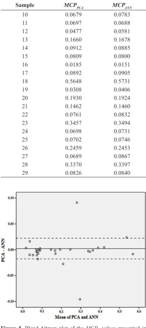
To compare ANN and PCA techniques to estimate
the MCPN, the Bland-Altman plot was considered and
presented in Figure 5. From that, it can be inferred that
the two methods of measurement agree suficiently close and that only three points were outside the 95% conidence interval, while most of them are near the
line of equality.
Discussion
MCP is a parameter introduced by Roque et al. (2013a) to provide a way to grade the trabecular bone fragility based on volume fraction, connectivity, tortuosity and elasticity, four fundamental quantities
Figure 3. Decrease of the error during the training of the neural network to estimate the MCPN.
Figure 4. MCP correlation between the PCA and ANN for the test samples.
Table 1.MCPN obtained by PCA and ANN algorithm for the 3 distal
radius samples by μCT.
Sample MCPPCA MCPANN
07 0.3247 0.2335
08 0.1951 0.2224
09 0.0450 0.0288
Table 2.MCPN obtained by PCA and ANN algorithm for the 6
vertebra samples by μCT.
Sample MCPPCA MCPANN
01 0.2475 0.3433
02 0.1655 0.1731
03 0.5487 0.5250
04 0.3908 0.3871
05 0.3617 0.3629
Filletti ÉR, Roque WL
that characterize the bone mechanical structure. In Roque et al. (2013a), Roque et al. (2013b) it has
been shown that the MCP can suitably be deined
for different trabecular bone sites using distinct image scanning devices and distinct mechanical test procedures.
The approach used in Roque et al. (2013a) is
based on the principal component analysis whose principal component deines the MCP equation. In this paper an artiicial neural network approach was applied to estimate the MCP based on two sets of
in vitro images samples from two distinct bone sites,
Table 3.MCPN obtained by PCA and ANN algorithm for the 20 distal
radius samples by MRI.
Sample MCPPCA MCPANN
10 0.0679 0.0783
11 0.0697 0.0688
12 0.0477 0.0581
13 0.1660 0.1678
14 0.0912 0.0885
15 0.0809 0.0800
16 0.0185 0.0151
17 0.0892 0.0905
18 0.5648 0.5731
19 0.0308 0.0406
20 0.1930 0.1924
21 0.1462 0.1460
22 0.0761 0.0832
23 0.3457 0.3494
24 0.0698 0.0731
25 0.0702 0.0746
26 0.2459 0.2453
27 0.0689 0.0867
28 0.3370 0.3397
29 0.0826 0.0840
Figure 5. Bland-Altman plot of the MCPN values presented in
Tables 1, 2 and 3.
L3 vertebrae and distal radius, and one set of in vivo
MRI distal radius samples. The results presented here
have shown the potentiality of the ANN to estimate the MCP taking into account different bone sample
sites, distinct imagery devices and the subject form as in vivo or in vitro.
The normalized MCP was estimated by both approaches and the results were compared by means of the Bland-Altman plot, which has shown that these techniques provide very similar results. In other words, the ANN performs essentially as good as the PCA to
estimate the MCPN, within the limits of agreement.
Of course, as neither is considered the gold standard technique to estimate the MCPN, as much as the
results are concerned, the ANN can suitably be used
to estimate the MCP.
Overall, in this paper an ANN was used to estimate the mechanical competence parameter based on μCT
and MRI image samples of vertebrae and distal radius
bones, together. The ANN predicted very well the MCP for a set of 38 test data composed of 6 vertebrae and 32 distal radius samples. The correlation between the MCP evaluated by the PCA and ANN is quite high
(R2 = 0.97) and the Bland-Altman analysis indicates
that both approaches are comparable within 95% conidence interval.
The ANN technique has shown to be a good
alternative to estimate the MCP, avoiding the cost of
the PCA, which requires the individual computation
of the MCP for each cohort. Of course, further
studies are required to investigate whether a unique ANN can be applied to estimate the MCPN from any
trabecular bone site, as in this paper only two sites were investigated, and also independently of the
imagery technique.
Acknowledgements
The authors thank Dr. Zbislaw Tabor for allowing us to make use of the set of μCT vertebral samples
and Dr. Angel Alberich-Bayarri for providing the MRI in vivo distal radius samples.
References
Arcaro K. Caracterização geométrica e topológica da competência mecânica no estudo da estrutura trabecular [thesis]. Porto Alegre: Universidade Federal do Rio Grande do Sul; 2013.
Christopher JJ, Ramakrishnan S. Assessment and classification of mechanical strength components of human femur trabecular bone using digital image processing and neural networks. Journal of Mechanics in Medicine and Biology. 2007; 7(3):315-24. http://dx.doi.org/10.1142/S0219519407002339.
Dimai HP, Redlich K, Peretz M, Borgström F, Siebert U, Mahlich J. Economic burden of osteoporotic fractures in Austria. Health Economics Review. 2012; 2(1):12. http:// dx.doi.org/10.1186/2191-1991-2-12. PMid:22827971. Filletti ER, Roque WL. Neural network prediction of the trabecular bone mechanical competence parameter. In: Braidot A, Hadad A, editors. IFMBE Proceedings; 2014 Oct 29-31; Paraná. Cham: Springer International Publishing; 2015. v. 49, p. 226-29.
Gregory JS, Junold RM, Undrill PE, Aspden RM. Analysis of trabecular bone structure using fourier transforms and neural networks. IEEE Transactions on Information Technology in Biomedicine. 1999; 3(4):289-94. http:// dx.doi.org/10.1109/4233.809173. PMid:10719479. Hambli R. Multiscale prediction of crack density and crack length accumulation in trabecular bone based on neural networks and nite element simulation. International Journal for Numerical Methods in Biomedical Engineering. 2011; 27(4):461-75. http://dx.doi.org/10.1002/cnm.1413. Haykin S. Neural networks: a comprehensive foundation. 2nd ed. New Jersey: Prentice Hall; 1999.
Jenkins WM. An introduction to neural computing for the structural engineer. Structural Engineering. 1997; 75(3):38-41. Jolliffe IT. Principal component analysis. 2nd ed. New York: Springer; 2002.
Nafey AS. Neural network based correlation for critical heat flux in steam-water flows. International Journal of Thermal Sciences. 2009; 48(12):2264-70. http://dx.doi. org/10.1016/j.ijthermalsci.2009.04.010.
Niemi H, Bulsari A, Palosaari S. Simulation of membrane separation by neural networks. Journal of Membrane Science. 1995; 102:185-91. http://dx.doi.org/10.1016/0376-7388(94)00314-O.
Roque WL, Alberich-Bayarri A. Tortuosity influence on the trabecular bone elasticity and mechanical competence. In: Tavares JMRS, Jorge RN, editors. Developments in medical image processing and computational vision, lecture notes in computational vision and biomechanics. Cham: Springer; 2015. v. 19, p. 173-91.
Roque WL, Arcaro K, Alberich-Bayarri A. Mechanical competence of bone: a new parameter to grade trabecular bone fragility from tortuosity and elasticity. IEEE Transactions on Biomedical Engineering. 2013a; 60(5):1363-70. http:// dx.doi.org/10.1109/TBME.2012.2234457. PMid:23268378. Roque WL, Arcaro K, Alberich-Bayarri A and Tabor Z. An investigation of the mechanical competence parameter to grade the trabecular bone fragility. In: Tavares JMRS, Jorge RN, editors. Proceedings of the 4th Computational Vision and Medical Image Processing; 2013 Oct 14-16; Funchal. Leiden: CRC Press; 2013b; p. 387-92.
Authors
Érica Regina Filletti1*, Waldir Leite Roque2
1 Departamento de Físico-Química, Instituto de Química, Universidade Estadual Paulista – UNESP, Rua Prof. Francisco
Degni, 55, Bairro Quitandinha, CEP 14800-900, Araraquara, SP, Brazil.
2 Departamento de Computação Cientíica, Centro de Informática, Universidade Federal da Paraíba – UFPB, João Pessoa,