Abstract
This study analyzes the fourth-order nonlinear free vibration of a Timoshenko beam. We discretize the governing differential equa-tion by Galerkin’s procedure and then apply the homotopy analy-sis method (HAM) to the obtained ordinary differential equation of the generalized coordinate. We derive novel analytical solutions for the nonlinear natural frequency and displacement to investi-gate the effects of rotary inertia, shear deformation, pre-tensile loads and slenderness ratios on the beam. In comparison to results achieved by perturbation techniques, this study demonstrates that a first-order approximation of HAM leads to highly accurate solu-tions, valid for a wide range of amplitude vibrasolu-tions, of a high-order strongly nonlinear problem.
Keywords
strongly nonlinear vibration, homotopy analysis method, Galerkin method, Timoshenko beam, nonlinear natural frequency
Nonlinear Vibrations of Cantilever Timoshenko
Beams: A Homotopy Analysis
1 INTRODUCTION
This study presents a closed-form analytical solution for a thick beam considering the Timoshenko formulation for various values of the relevant design parameters applying the homotopy analysis method (HAM), introduced by Liao (1998; 2003; 2004; 2007; 2009). Making no use of small parame-ters it allows us to consider the general nonlinear system for small as well as large amplitude vibra-tions. Thus it overcomes the requirement for perturbation techniques, such as the multiple scales method, to model the problem as a weakly nonlinear system involving perturbation quantities. To ensure accurate results the partial differential equation is first discretized by the Galerkin procedure before HAM is applied to the obtained nonlinear ordinary differential equation.
Previously, Ramezani et al. (2006) provided a second-order perturbation solution for a doubly clamped Timoshenko microbeam using the multiple scales method. Moeenfard et al. (2011) also analyzed this problem by applying the homotopy perturbation method. Foda (1999) analyzed the same problem in macro-scale with perturbation methods considering the pinned boundary
condi-Shahram Shahlaei-Far Airton Nabarrete* José Manoel Balthazar
Instituto Tecnológico de Aeronáutica, Praça Marechal Eduardo Gomes 50, São José dos Campos, SP, 12228-900, Brazil
*Corresponding author: [email protected]
http://dx.doi.org/10.1590/1679-78252766
tion. A comparison to results from Ramezani et al. (2006) for the doubly clamped case shows the formidable accuracy of HAM. Furthermore, a parametric study discusses the effects of applied ten-sile loads and slenderness ratios on the large amplitude vibration of the cantilever Timoshenko beam. The analysis also addresses the effects of rotary inertia and shear deformation on the nonlin-ear natural frequency.
The homotopy analysis method is a nonperturbative analytical technique for obtaining series so-lutions to nonlinear equations. Its freedom to choose different base functions to approximate a non-linear problem and its ability to control the convergence of the solution series have been very ad-vantageous in solving highly nonlinear problems in science and engineering (Hoseini et al., 2008; Hoshyar et al., 2015; Mastroberardino, 2011; Mehrizi et al., 2012; Mustafa et al., 2012; Pirbodaghi and Hoseini, 2009; Pirbodaghi et al., 2009; Qian et al., 2011; Ray and Sahoo, 2015; Sedighi et al., 2012; Wen and Cao, 2007; Wu et al., 2012).
2 GOVERNING DIFFERENTIAL EQUATION
The nonlinear free vibration of a thick beam considering the Timoshenko formulation for the mid-plane stretching and the effects of rotary inertia and shear deformation was first reviewed by Ramezani et al. (2006). In that article, a full description of the problem was presented in which the governing equation was derived as
4 2 4 2 2 4
2
4 2 2 2 4
2 4 2 4
2 4 2 2 0
w w mEI w m r w
EI m mr
AG AG
x t x t t
w EI w mr w
N
AG AG
x x x t
k k
k k
æ ö
¶ + ¶ -ç + ÷÷ ¶ + 
-ç ÷
ç ÷
è ø
¶ ¶ ¶ ¶ 
é¶ ¶ ¶ ù
ê - + ú
ê¶ ¶ ¶ ¶ ú
ê ú
ë û =
(1)
where
w
is the transverse displacement,x
is the axial coordinate of the beam and t is the time. As constant terms, E is the modulus of elasticity, G is the shear modulus, A is the cross-section area, I is the second moment of area of the cross section with respect to the bending axis,r
is the radius of gyration of the beam cross section given by r2 =I A,m
is mass per unit length andk
is the shear correction factor that depends only on the geometric properties of the cross section of the beam.
The last bracketed terms in Eq. 1 represent the nonlinearity due to large amplitudes caused by the axial force N, which is given by
2 0 2 0
L
EA w
N N dx
L x
æ¶ ÷ö ç
= + çç ÷÷÷
è¶ ø
ò
(2)where N0 is the pre-tensile load and L is the length of the beam. For convenience, we take the nondimensional quantities
2
1 ˆ
ˆ
ˆ x, w and t , with m
x w t T
L L T b EI
where b is the numerical solution for cosbLcoshbL= -1 of a corresponding Euler-Bernoulli beam
(Meirovitch, 2001).
Considering bL = bˆ, Eqs. (1) and (2) are rewritten in nondimensional form
2 4
4 4 4 2
4 8 4
4 2 2 4 2
2 2 4 4 4
4 4
ˆ ˆ ˆ ˆ ˆ ˆ ˆ
1
ˆ ˆ ˆ
ˆ ˆ
ˆ ˆ ˆ
ˆ ˆ
w r E w r E w w
G L G
x x t t t
N L r E w r E w
EA r L x G
L
G L
b b b
k k
b
k k
æ ö æ ö æ ö æ ö
¶ - ç ÷÷ ç + ÷÷ ¶ + ç ÷÷ ç ÷÷¶ + ¶ +
ç ÷ ç ÷ ç ÷ ç ÷
ç ÷ ç ÷ ç ÷ ç ÷
è ø è ø è ø è ø
¶ ¶ ¶ ¶ 
æ ö æ ö æ÷ ÷ ö÷¶ æ ö æ÷ ö÷ 
ç ÷ ç ÷ ç ÷ - ç ÷ ç ÷
ç ÷ ç ÷ ç ÷ ç ÷ ç ÷
ç ÷ ç ÷ ç ÷ ç ÷ ç ÷
è ø è ø è ø¶ è ø è ø
2 2 2 2
ˆ 0
ˆ ˆ
w
x t x
æ ö÷
ç ¶ ÷
ç - ÷=
ç ÷
ç ¶ ¶ ÷÷
çè ø (4) 2 1 0 0 ˆ ˆ ˆ 2 EA w
N N dx
x
æ¶ ÷ö ç
= + çç ÷÷÷
è¶ ø
ò
(5)The boundary conditions for a cantilever beam formulated in this research are
2 3
2 3
ˆ
ˆ 0 , 0 at ˆ 0 ˆ
ˆ ˆ
ˆ 0 , 0 at 1
ˆ ˆ w w x x w w x x x ¶ = = = ¶ ¶ = ¶ = = ¶ ¶ (6)
Hereafter the caret on all the variables is dropped for convenience.
The nondimensional transverse displacement is here approximated as w x t( , )= Q( )x W t( ) where
( )x
Q is the normalized mode shape of the corresponding cantilever Euler-Bernoulli beam and W t( )
the corresponding time-dependent generalized coordinate.
The average over the space variable is applied to reduce Eq. (4) to an ordinary differential equation. Multiplying Eq. (4) by Q( )x and integrating it over the interval of [0,1], the governing
nonlinear differential equation is derived as
2 3
1 2 3 4
( ) 0
W+ a +aW W +aW +aW = (7)
where the dot represents differentiation with respect to time t and the parameters aj for
1, 2, 3, 4
j = are given by
2 2
0
1 4 1 2 4 3 1
1 1
2
4 4
0 0
3 2 1 4 8 3 2 3 1
1 1
2 2
8
1 , ,
2
, 2
N
G G
E E EA
N N
G G G
E EA E EA E
r k k r
a r d a d d
b b
r k k r k
a d r d a d d r d d
b b
æ ö÷ æ ö æ ö
ç ÷ ç ÷÷ ç ÷÷
ç ÷ ç ÷ ç ÷
ç ÷ ç ÷ ç ÷
ç è ø è ø
è ø
é æç öù÷
ê ÷ú
= ê - çç + + ÷÷ú =
-çè ø
ë û
é æç öù÷ æç ö÷
ê ÷ú
= ëê + - çèçç ÷ø÷ûú = èçç - ÷ø÷÷
(8)
( )
1 1
1 2
0 0
1
2 2 3
1 1 0
0 0
2
, ,
dx dx
dx
dx dx
d = Q Q¢¢ d = Q¢¢¢¢Q d = Q¢
Q Q
ò
ò
ò
ò
ò
(9)where the prime denotes differentiation with respect to the spatial variable x. Let t =wtdenote a new time scale. Under the transformation
, V( ) ( )
t W t
t =w t = (10)
Eq. (7) becomes
4 2
4 2 2 3
1 2 3 4
4 2
( ) ( )
( ) ( ) ( ) 0
d V d V
V V V
d d
t t
w w a a t a t a t
t t
é ù
+ êë + úû + + = (11)
The nonlinear ordinary differential equation is subject to the following initial conditions
2 3
max
2 3
(0) (0) (0)
(0) W , dV d V d V 0
V
L dt dt dt
= = = = (12)
where Wmax is the amplitude at the free end of the beam.
3 HOMOTOPY ANALYSIS METHOD
The homotopy analysis method is an analytical technique for solving general nonlinear differential equations. It transforms a nonlinear differential equation into an infinite number of linear differen-tial equations embedding an auxiliary parameter q Î[0,1]. As increases from 0 to 1, the solution varies from the initial guess to the exact solution (Liao, 2003).
Free oscillation without damping is a periodic motion and can be expressed by the following set of base functions
{cos(mt) |m =1,2, 3, }¼ (13)
such that the general solution is given as
1
( ) cos( )
i i
V t g mt
¥
=
=
å
(14)wheregiare coefficients to be determined. We choose the initial guess
0
9 1
( ) cos( ) cos(3 )
8 8
V t = D t - D t with D Wmax Wmax s
L h r
= = , s h 3.46416
r »
› (15)
4 2
4 2 2 3
1 2 3 4
4 2
; ( ; )
( ; ),q f t( q) [ ( ; )]q f t q ( ; )q ( ;q)
f t w w w a a f t a f t a f t
t t
¶ 
é ù = + + + +
ë û ¶ 
(16)
where q is an embedding parameter and f t( ;q) is a function of t and q. To ensure the rule of
solution expression given by Eq. (14) we choose the linear operator to be
4 2
4
4 2
(
( ; ) )
( ; )q f t q f t;q
f t w
t t
æ¶ ¶ ö÷
ç
é ù = çç + ÷÷
ë û çè ¶ ¶ ÷÷ø
(17)
with the property
1 2 3cos( ) 4sin( ) 0
C C t C t C t
é + + + ù =
ë û
(18)
where C C C1, 2, 3 and C4 are constants of integration.
Now, we can construct a homotopy
0 0 0 0
( ( ; );f t q V( ),t H( )t ,c q, )=(1-q) éëf t( ; )q -V ( )t ûù-qc H( )t éëf t( ; )q ,wùû
H
(19)where c0 ¹0 is the convergence-control parameter and H( )t a nonzero auxiliary function. Enforc-ing the homotopy in Eq. (19) to be zero, i.e.
H
( ( ; );f tq V0( )t ,H( ),t c q0, )=0, we obtain the zero-order deformation equation0 0
(1-q)ëéf t( ; )q -V (t)ûù =qc H(t) éëf t( ; )q ,wùû (20)
In Eq. (20), for q = 0 and q =1 we have, respectively,
0
( ; 0) V ( )
f t = t and f t( ;1)=V( )t (21)
Thus, the function f t( ;q) varies from the initial guess V0( )t to the desired solution as q varies from 0 to 1. The Taylor expansions of f t( ;q) with respect to q is
0
1
( ; ) ( ) ( ) m m m
q V V q
f t t t
¥
=
= +
å
(22)where
0
( | ) ; 1
( ) !
m
m m q
q V
m q
f t
t = ¶ =
¶ (23)
Choosing properly the linear operator, the initial guess, the auxiliary function H( )t and the convergence-control parameter c0, the series in Eq. (22) converges when q =1, such that
0
1
( )
( ) m( )
m
V t V t V t
¥
=
Differentiating the zero-order equation (20) with respect to q and setting q = 0, the first-order deformation equation is obtained as
1( ) 0 ( ) 0( ),
V t c H t V t w
é ù = é ù
ë û ë û
(25)
subject to the initial conditions
1 1
(0)
(0) dV 0
V
dt
= = (26)
For the nonzero auxiliary function H( )t to obey the rule of solution expression and the rule of
coefficient ergodicity, we choose it to be
( ) co (2s )
H t = kt (27)
where k is an integer. It can be determined uniquely as H( )t =1. As a result, Eq. (25) becomes
4 2 4 2
1 1 0 0
4 2 4 2
4 4 2 2 3
0 1 2 0 3 0 4 0
( ) ( ) ( ) ( )
( ( )) ( ) ( )
d V d V d V d V
d d c d V d V V
w t t w t w t
t t t a a t t a t a t
æ ö÷ é ù
ç ÷ ê ú
ç ÷
ç ÷ ê ú
ç ÷
è + ø= êë + + + + ûú
0 1,0[ ( 0, )cos( ) 1,1( , ) cos(3 )0 1,2( , ) c0 os(5 )
c b V w t b V w t b V w t
= + + +
1,3( , ) cos(7 )0 1,4( , )cos(9 )]0
b V w t +b V w t
(28)
where the coefficients b1,i( , )V0 w , i = 0,1, 2, 3, 4 are obtained as
4 2 3 3
1,0 1 2 3 4
9 9 819 9 999
8 8 1024 8 1024
b = w D-w çççæ aD + aD ö÷÷ +÷÷ aD+ aD
è ø
4 2 3 3
1,1 1 2 3 4
81 9 135 1 15
8 8 256 8 128
b = - w D-w çççæ aD + aD ö÷÷ -÷÷ aD+ aD
è ø
2 3 3
1,2 2 4
45 27
128 256
b = w aD - aD
2 3 3
1,3 2 4
171 27
2048 2048
b = - w aD + a D
2 3 3
1,4 2 4
9 1
2048 2048
b = w aD - a D
(29)
According to the property of the linear operator, if the term cos( )t exists on the right side of Eq. (28), the secular term tsin( )t will appear in the final solution. Thus, to obey the rule of
solu-tion expression, the coefficient b1,0 has to be equal to zero. Solving the algebraic equation for the
nonlinear natural frequency, it is obtained as
1 2 2
4 1
91 1
256 2
nl D F
w =ççææçççç a + a ö÷÷ - ÷÷÷ ö÷÷÷
with
1
2 2
2 2
4 1 3 4
91 1 111
256 2 128
F aD a a aD
ææ ö æ ö÷ö
çç ÷ ç ÷÷
ç ÷
=ççèçèçç + ÷÷ -÷ø èçç + ÷÷÷÷ø÷÷ø (31)
There are two sinusoidal modes of different frequencies. For our purposes we consider the lower fundamental frequency which is associated with bending deformation.
Finally, solving Eq. (28) for the displacement of the beam, the general solution of Eqs. (11) and (12) is achieved as
*
1( ) 1( ) 1 2 3cos( ) 4sin( )
V t =V t +C +C t +C t +C t
4 1, 4 1 0 3 2 2 1 cos((2 1) ) cos( )
(2 1) ((2 1) )
n n nl c n C b n n
w = t t
= +
+ + - +
å
1,1 1,2
0
4 72(cos(3 ) cos( )) 600(cos(5 ) cos( ))
nl
b b
c
t t t t
w
æç ç
= - +
-çççè
1,3 (cos(7 ) cos ) 1,4 cos(9 ) cos( )
2352 ( ) 6480( )
b b
t t t t ö÷÷
+ - + - ÷÷÷ø
(32)
where * 1( )
V t is the special solution, C1 =C2 =C4 =0to comply with the rule of solution expres-sion and C3 is obtained from the initial conditions given in Eq. (24).
Thus, with Eq. (24) the first-order approximation of W t( )becomes
0 1 )
) (
( ( ) V ( ) V
W t =V t » t + t
1,1 1,2 1,3 1,4 1,1
0 0
4 4
9 1
cos cos(3 )
8 72 600 2352 6480 ( nl ) 8 72 nl
nl nl
b b b b b
c c
D w t D w t
w w
æ æ öö÷÷ æ ö÷
ç ç ÷÷ ç ÷
ç ç ç
=çç - çç + + + ÷÷÷÷÷÷ -çç - ÷÷÷
ç ç ç
è è øø è ø
1,2 1,3 1,4
0
4 600cos(5 nl ) 2352cos(7 nl ) 6480cos(9 nl )
nl
b b b
c
t t t
w w w
w
æ ö÷
ç ÷
ç
+ çç + + ÷÷÷
çè ø
(33)
4 RESULTS
The effects of rotary inertia and shear deformation as well as vibration amplitude for various design parameters on the nonlinear natural frequency of thick and short beams for the clamped-free boundary condition are discussed in this section. The accuracy of a first-order approximation of the homotopy analysis method is confirmed by comparison with results obtained from Ramezani et al. (2006) for clamped-clamped microbeams. The geometric and material properties of the Timoshenko beam in consideration are given in Table 1. For purposes of comparison the natural linear frequency
l
w of the Euler-Bernoulli beam theory, given by
2 2 0 2 4 1 1 l N L EA r w d b d
æ æ ö ö÷
ç ç ÷ ÷
ç ÷
= çç - çç ÷÷÷ ÷÷
è ø ÷
Property E G r A k
Value 169 GPa 66 GPa 2330 kg/m³ 90 μm² 5/6
Table 1: Geometric and material properties of the Timoshenko beam.
In Figure 1 we observe that a first-order approximation of the HAM provides excellent agree-ment with results achieved by Ramezani et al. (2006) for doubly clamped microbeams. Three slen-derness ratios have been considered ranging from thick
(
L r =20)
to slender beams(
L r =100)
.For the calculation, the first normalized mode of vibration Q( )x and the value for b =b1 have been
adequately adjusted with respect to the boundary condition.
(a) (b)
(c)
Figure 1: Nonlinear frequency of clamped-clamped beam for different slenderness ratios.
The rest of our discussion deals with cantilever Timoshenko beams. Applying HAM to a nonlin-ear problem results in a family of solution series which depend on the convergence-control parame-ter. The optimal value is obtained by minimizing the square residual error of the governing equa-tion for a given order of approximaequa-tion. For a first-order approximaequa-tion, Figure 2 presents the time-domain response of the nonlinear system in accurate agreement with numerical results. Considering
10,20, 30
L r = the length-to-thickness ratios are L h »2.8867, 5.7734, 8.6601, respectively. The
stretching effect occurring at the beam’s centerline causes the nonlinear frequency to increase
0 0.2 0.4 0.6 0.8 1
0.9 1 1.1 1.2 1.3
Wmax /h nl
/
l
Present results Ramezani et al. (2006)
L/r = 20
0 0.2 0.4 0.6 0.8 1
0.9 1 1,1 1,2 1,3
Wmax /h nl
/
l
Present results Ramezani et al. (2006)
L/r = 50
0 0.2 0.4 0.6 0.8 1
0.9 1 1.1 1.2 1.3
Wmax /h nl
/
l
Present results Ramezani et al. (2006)
considerably (over 70%) with the increase of the initial deflection Wmax h as seen in Figure 3. At small deflections, there are no significant discrepancies between the linear and nonlinear model which suggests that for weak nonlinearity linear models would give sufficiently reasonable estimates.
Figure 2: Time response of clamped-free beam for c0 = 0.0048.
(a) (b)
(c)
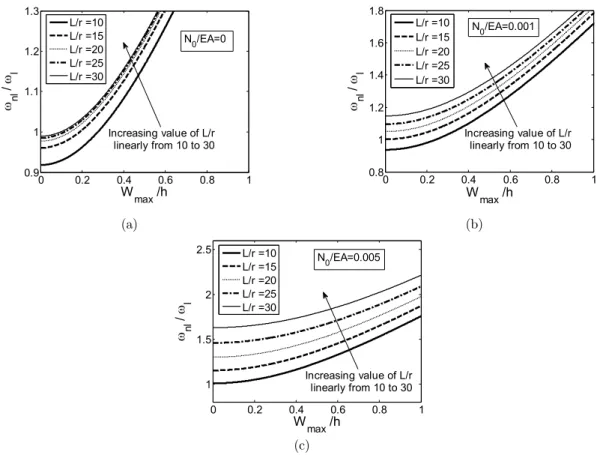
Figure 3: Nonlinear frequency of clamped-free beam for varying slenderness ratios.
0 2 4 6 8 10
-0.2 -0.1 0 0.1 0.2 0.3
Time t
W(
t)
Present results Numerical results
Wmax/h=1, L/r=20, N0/EA=0, G/E=0.3254
0 0.2 0.4 0.6 0.8 1
0.9 1 1.1 1.2 1.3
Wmax /h nl
/
l
L/r =10 L/r =15 L/r =20 L/r =25 L/r =30
Increasing value of L/r linearly from 10 to 30 N0/EA=0
0 0.2 0.4 0.6 0.8 1
0.8 1 1.2 1.4 1.6 1.8
Wmax /h / nl
l
L/r =10 L/r =15 L/r =20 L/r =25 L/r =30
Increasing value of L/r linearly from 10 to 30
N0/EA=0.001
0 0.2 0.4 0.6 0.8 1
1 1.5 2 2.5
Wmax /h nl
/
l
L/r =10 L/r =15 L/r =20 L/r =25 L/r =30
Increasing value of L/r linearly from 10 to 30
Moreover, Figure 3 depicts the influence of the slenderness ratio on the nonlinear frequency for different values of the pre-tensile load. At small values of Wmax h, increasing L r linearly, the nonlinear frequency increases considerably for all values of the pre-tensile load, whereby the nonlin-earity effect for lower values of L/r is more substantial. On the other hand, for large values of
max
W h, the difference between the nonlinear frequencies corresponding to different slenderness
ratios becomes smaller.
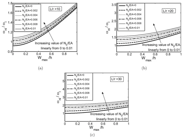
For given slenderness ratios the influence of varying pre-tensile loads is demonstrated in Figure 4. The nonlinear frequency of the beam is augmented when linearly increasing pre-tensile axial loads are applied having greater impact at small values of Wmax h.
(a) (b)
(c)
Figure 4: Nonlinear frequency of clamped-free beam for varying pre-tensile loads.
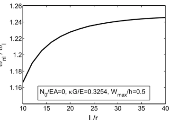
In Figures 5 and 6 the effects of rotary inertia and shear deformation on the large amplitude vi-bration are depicted, where the nonlinear frequency is plotted against kG E and L r, respectively.
In both cases, the nonlinear frequency converges to a definite value when kG E and L r are being
increased, respectively. Thus for slender beams the effects of rotary inertia and shear deformation are negligible as expected. On the other hand, for any thick beam analysis they must be included.
0 0.2 0.4 0.6 0.8 1
0.8 1 1.2 1.4 1.6 1.8
Wmax /h nl
/
l
N0/EA=0 N0/EA=0.002 N0/EA=0.004 N0/EA=0.006 N0/EA=0.008 N0/EA=0.01
Increasing value of N0/EA linearly from 0 to 0.01
L/r =10
0 0.2 0.4 0.6 0.8 1
1 1.5 2 2.5 3 3.5
Wmax /h nl
/
l
N0/EA=0 N0/EA=0.002 N0/EA=0.004 N0/EA=0.006 N0/EA=0.008 N0/EA=0.01
Increasing value of N0/EA linearly from 0 to 0.01
L/r =20
0 0.2 0.4 0.6 0.8 1
1 2 3 4 5
Wmax /h nl
/
l
N0/EA=0 N0/EA=0.002 N0/EA=0.004 N0/EA=0.006 N0/EA=0.008 N0/EA=0.01
L/r =30
Figure 5: Influence of rotary inertia on nonlinear frequency of clamped-free beam.
Figure 6: Influence of shear deformation on nonlinear frequency of clamped-free beam.
5 CONCLUSIONS
The present study analyzed free nonlinear vibrations of Timoshenko beams by means of the ho-motopy analysis method to yield straightforward closed-form expressions for the nonlinear natural frequency and the generalized coordinate corresponding to the first spatial mode. The efficiency and accuracy of the method was demonstrated by a comparison between solutions obtained by HAM and perturbation methods for the clamped-clamped boundary condition.
In the case of cantilever Timoshenko beams, we investigated the effects of rotary inertia and shear deformation as well as the influence of design parameters such as the slenderness ratio and pre-tensile loads on the nonlinear natural frequency. Higher natural frequencies are observed for the nonlinear model when pre-tensile loads or slenderness ratios are increased. By augmenting the effect of shear deformation and rotary inertia, respectively, the nonlinear natural frequency of the beam rises significantly and converges to a definite value. Moreover, it is shown that the time response of the nonlinear system agrees accurately with numerical results.
Unlike perturbation methods, HAM is valid for a wide range of parameters and vibration ampli-tudes as it does not require small parameters for its analysis and the study shows that a first-order homotopy approximation efficiently obtains accurate analytical results for a high-order strongly nonlinear problem.
References
Foda, M.A., (1999). Influence of shear deformation and rotary inertia on nonlinear free vibration of a beam with pinned ends. Computers & Structures 71:663–670.
Hoseini, S.H., Pirbodaghi, T., Asghari, M., Farrahi, G.H., Ahmadian, M.T., (2008). Nonlinear free vibration of con-servative oscillators with inertia and static type cubic nonlinearities using homotopy analysis method. Journal of Sound and Vibration 316:263–273.
Hoshyar, H.A., Ganji, D.D., Borran, A.R., Falahati, M., (2015). Flow behavior of unsteady incompressible Newtoni-an fluid between two parallel plates via homotopy Newtoni-analysis method. Latin AmericNewtoni-an Journal of Solids Newtoni-and Structures 12:1859–1869.
0 0.05 0.1 0.15 0.2 0.25 0.3 0.4
0.6 0.8 1 1.2 1.4
G/E / nl
l
N0/EA=0, L/r=20, Wmax/h=0.5
10 15 20 25 30 35 40
1.16 1.18 1.2 1.22 1.24 1.26
L/r nl
/
l
Liao, S.J. (2003). Beyond perturbation: Introduction to homotopy analysis method, Chapman&Hall/CRC Press (Boca Raton).
Liao, S.J., (2004). On the homotopy analysis method for nonlinear problems. Applied Mathematics and Computation 147:499–513.
Liao, S.J., (2009). Notes on the homotopy analysis method: Some definitions and theorems. Communications in Nonlinear Science and Numerical Simulation 14:983–997.
Liao, S.J., Cheung, A.T., (1998). Application of homotopy analysis method in nonlinear oscillations. ASME Journal of Applied Mechanics 65:914–922.
Liao, S.J., Tan, Y., (2007). A general approach to obtain series solutions of nonlinear differential equations. Studies in Applied Mathematics 119:297–355.
Mastroberardino, A., (2011). Homotopy analysis method applied to electrohydrodynamic flow. Communications in Nonlinear Science and Numerical Simulation 16:2730–2736.
Mehrizi, A.A., Vazifeshenas, Y., Domairry, G., (2012). New analysis of natural convection boundary layer flow on a horizontal plate with variable wall temperature. Journal of Theoretical and Applied Mechanics 50(4):1001–1010. Meirovitch, L., (2001). Fundamentals of Vibrations, McGraw-Hill (New York).
Moeenfard, H., Mojahedi, M., Ahmadian, M.T., (2011). A homotopy perturbation analysis of nonlinear free vibration of Timoshenko microbeams. Journal of Mechanical Science and Technology 35(3):557–565.
Mustafa, M., Hayat, T., Hendi, A.A., (2012). Influence of melting heat transfer in the stagnation-point flow of a Jeffrey fluid in the presence of viscous dissipation. ASME Journal of Applied Mechanics 79(2):4501–4505.
Pirbodaghi, T., Ahmadian, M.T., Fesanghary, M., (2009). On the homotopy analysis method for non-linear vibration of beams. Mechanics Research Communications 36(2):143–148.
Pirbodaghi, T., Hoseini, S., (2009). Nonlinear free vibration of a symmetrically conservative two-mass system with cubic nonlinearity. ASME Journal of Computational and Nonlinear Dynamics 5(1):1006–1011.
Qian, Y. H., Lai, S. K., Zhang, W., Xiang, Y., (2011), Study on asymptotic analytical solutions using HAM for strongly nonlinear vibrations of a restrained cantilever beam with an intermediate lumped mass. Numerical Algo-rithm 58:293–314.
Ramezani, A., Alasty, A., Akbari, J., (2006). Effects of rotary inertia and shear deformation on nonlinear free vibra-tion of microbeams. ASME Journal of Vibravibra-tion and Acoustics 128(5):611–615.
Ray, S.S., Sahoo, S., (2015). Traveling wave solutions to Riesz time-fractional Camassa–Holm equation in modeling for shallow-water waves. ASME Journal of Computational and Nonlinear Dynamics 10(6):1026–1030.
Sedighi, H.M., Shirazi, K.H., Zare, J., (2012). An analytic solution of transversal oscillation of quintic non-linear beam with homotopy analysis method. International Journal of Non-linear Mechanics 47:777–784.
Wen, J., Cao, Z., (2007). Sub-harmonic resonances of nonlinear oscillations with parametric excitation by means of the homotopy analysis method. Physics Letters A 371:427–431.